Article

Source Enumeration Approaches Using Eigenvalue Gaps and Machine Learning Based Threshold for Direction-of-Arrival Estimation

1
Electronic Warfare Research Center, Gwangju Institute of Science and Technology, Gwangju 61005, Korea
2
School of Electrical Engineering and Computer Science, Gwangju Institute of Science and Technology, Gwangju 61005, Korea
3
Electronic Warfare R&D Center, LIG Nex1 Co., Ltd., Yongin-si 16911, Korea
4
2nd R&D Institute, Agency for Defense Development, Daejeon 34186, Korea
*
Author to whom correspondence should be addressed.
Appl. Sci. 2021, 11(4), 1942; https://doi.org/10.3390/app11041942
Submission received: 12 January 2021 / Revised: 17 February 2021 / Accepted: 18 February 2021 / Published: 23 February 2021
(This article belongs to the Special Issue Recent Advances in Electronic Warfare Networks and Scenarios Ⅱ)

Abstract

:
Source enumeration is an important procedure for radio direction-of-arrival finding in the multiple signal classification (MUSIC) algorithm. The most widely used source enumeration approaches are based on the eigenvalues themselves of the covariance matrix obtained from the received signal. However, they have shortcomings such as the imperfect accuracy even at a high signal-to-noise ratio (SNR), the poor performance at low SNR, and the limited detection number of sources. This paper proposestwo source enumeration approaches using the ratio of eigenvalue gaps and the threshold trained by a machine learning based clustering algorithm for gaps of normalized eigenvalues, respectively. In the first approach, a criterion formula derived with eigenvalue gaps is used to determine the number of sources, where the formula has maximum value. In the second approach, datasets of normalized eigenvalue gaps are generated for the machine learning based clustering algorithm and the optimal threshold for estimation of the number of sources are derived, which minimizes source enumeration error probability. Simulation results show that our proposed approaches are superior to the conventional approaches from both the estimation accuracy and numerical detectability extent points of view. The results demonstrate that the second proposed approach has the feasibility to improve source enumeration performance if appropriate learning datasets are sufficiently provided.

1. Introduction

In the battlefield of modern and future warfare, the importance of electronic warfare (EW) is increasing. EW consists of an electronic attack (EA), which controls the enemy’s electromagnetic spectrum; electronic protection (EP), which is used for defense; and electronic warfare support (ES), which supports tasks such as surveillance and reconnaissance [1]. Direction-of-arrival (DOA) is a key process of ES for locating the signal sources of the enemies [2,3]. DOA is used not only for EW applications but also in many applications such as radar, sonar, wireless communication, radio astronomy, and satellite communications [4].
Algorithms such as multiple signal classification (MUSIC) [5] and estimation of the signal parameters via rotational invariance techniques (ESPRIT) [6] are widely used for the DOA estimation, which are subspace-based techniques. They divide the covariance matrix of the received signals into two subspaces: signal–subspace and noise–subspace, and estimate the DOA of the received signals utilizing the orthogonal relation between the signal–subspace and noise–subspace [7,8,9]. Although the subspace-based techniques such as MUSIC and ESPRIT can estimate DOA with high-resolution, they need to know the exact number of sources to distinguish between the signal- and noise–subspace [10]. In practice, however, the number of sources is not known a priori; the source enumeration must be executed before the DOA techniques are performed. If we fail to estimate the exact number of sources, it will lead to a deterioration in the performance of the DOA estimation [11]. Therefore, the source enumeration is greatly important for DOA estimation.
There are two famous source enumeration approaches by information theoretic criteria: Akaike information criterion (AIC) and minimum description length (MDL) [12]. AIC has fairly good estimation accuracy at low signal-to-noise ratio (SNR) but does not reach perfect (100%) accuracy even at high SNR [13], while MDL has 100% accuracy at high SNR, but the performance is sharply and extremely degraded at a low level of SNR [14]. Another algorithm called a second order statistic of the eigenvalues (SORTE) [15] outperforms other approaches in estimation accuracy but its numerical detectability extent—the maximum number of source signal detection with a given array—is less than that of AIC and MDL [16].
In this paper, two approaches that use gaps of the eigenvalues for the covariance matrix obtained from the received multiple signals are proposed to overcome the poverties of the accuracy of AIC at high SNR and MDL at low SNR, and the limited detectability extent of source enumeration for SORTE. In the first approach, the source signals are enumerated with the criterion formula selection that is comprised of the ratio of the eigenvalues gaps. In the second approach, the threshold-based estimation using the machine learning approaches is proposed; the optimal threshold that minimizes the estimation error is derived by the machine learning based clustering algorithm. In the performance evaluation, AIC, MDL, SORTE, and our two proposed approaches are compared in terms of source enumeration accuracy in a wide range of SNR. Conclusively, simulation results demonstrate that the first approach has better performance than SORTE for the overall range of SNR, and our proposed approach can detect one more source than SORTE can. In addition, results show that the second proposed approach has fairly good performance and its performance can be further enhanced if the appropriate learning data are provided.
The main contributions of our study are summarized as follows:
  • Our proposed approach based on the criterion formula selection shows the better performance of source enumeration accuracy than SORTE for the overall range of SNR, and it can detect one more signal than SORTE can. In addition, the source enumerating criterion formula of the proposed approach is much simpler than that of SORTE.
  • To the best of our knowledge, this paper presents the first source enumeration approach based on the machine learning algorithm using gaps of eigenvalues. It is shown that our proposed machine learning based clustering approach has fairly good performances, and it also reveals the strong feasibility to improve its performance when the appropriate learning data are sufficiently supported for the designated SNR range.
  • While in most existing literature, the performances of source enumeration approaches are evaluated with predefined fixed parameters (e.g., the number of sources and the arrival angles of the sources), which results in the eigenvalues of the covariance matrix being fixed. In this paper, the performances for the cases with a comprehensive number of sources and arrival angle of the sources are compared in this paper. It is shown that our proposed approaches have comparatively good performances in the various scenario conditions of signal sources.
The remainder of this paper is organized as follows: Section 2 surveys related research studies on DOA estimation and source enumeration approaches. Section 3 presents our system model for the source enumeration. In Section 4, two source enumeration approaches based on the gap ratio criterion formula and threshold of eigenvalues gaps are proposed. Analyses through simulations are presented in Section 5, and conclusions are drawn in Section 6.

2. Related Works

In this section, previous works on DOA estimation and source enumeration are surveyed. Machine learning techniques are also introduced briefly and previous works applying machine learning to DOA estimation and source enumeration are presented.
Not only MUSIC and ESPRIT but also many DOA estimation studies are assuming that they know the number of signals a priori. Zuo et al. [17] proposed a subspace-based localization of far-field and near-field signals without eigendecomposition; they assume that the number of far-field and near-field signals are known when they state the problem formulation. Lonkeng and Zhuang [18] and Nie et al. [19] proposed a low-complexity and fast two-dimensional DOA estimation, where they are assuming the a priori knowledge of the number of signals. Yan et al. [20] proposed a reduced-complexity algorithm for DOA estimation exploiting only the real part of the covariance matrix of the array and showed that it can lead to a real-valued version of the MUSIC algorithm with no dependence on array configurations, while their basic assumptions include that the number of sources is known. Weng et al. [21] address the problem of DOA estimation with coprime arrays with the emphasis on reduced computational complexity while preserving estimation accuracy; the number of sources is also assumed to be known. As described above, the source enumeration is critical to many applications of DOA estimation.
There are a large number of studies on source enumeration approaches, and they can be classified into information theoretic based and threshold based approaches, etc. [14]. AIC and MDL, which are the information theoretic based approaches, are the most popular approaches for source enumeration. Wax and Kailath [12] are the first who applied AIC and MDL to detect the number of signals. These approaches use the eigenvalues of the covariance matrix and have advantages in which no subjective judgment (e.g., deciding on the threshold levels) is required in the decision process. However, AIC yields an inconsistent estimate that tends to overestimate the number of signals; hence, AIC does not reach 100% accuracy even at high SNR levels. Meanwhile, MDL has 100% accuracy at high SNR levels but has poor performance at low SNR levels [22]. Another eigenvalue-based approach named SORTE was proposed by He et al. [15] to detect the number of clusters; it also can be used to detect the number of signals and showed comparatively good estimation performances [23]. While AIC and MDL use the eigenvalues directly, SORTE uses the gaps of the eigenvalues; hence, SORTE cannot detect as many signals as AIC and MDL can—two less signals than AIC and MDL. Meanwhile, a threshold based approach named the eigenthreshold (ET) approach was proposed by Chen et al. [24]. ET detects the number of signals by setting the upper thresholds for the observed eigenvalues and then implementing a hypothesis testing procedure. Another threshold based approach, the eigen-increment threshold, was proposed by Hu et al. [25]. This approach is based on the assumption that, without the existence of the signals, the noise eigenvalues distribute approximately along a straight line; if the signals exist, it causes the increase of the eigenincrement on the boundary between two subspaces. Based on this observation, they proposed a single threshold concerning about the information of signal and noise strength, data length, and array size.
The studies on machine learning have attracted a great amount of attention over the past few years. Machine learning techniques can be divided into four categories: supervised, unsupervised, semi-supervised, and reinforcement learning [26]. Supervised learning uses a labeled training dataset to teach a model; after training, a new piece of unlabeled data can decide to be one of the trained labels according to the model. The widely-used supervised learning algorithms are k-Nearest neighbor, decision tree, random forest, and neural network, etc. Unlike supervised learning, unsupervised learning is not given the labeled training dataset; the patterns of the dataset are discovered by themselves. The widely-used unsupervised learning algorithms are k-Means clustering and a self-organizing map. Semi-supervised learning uses both labeled and unlabeled data, and reinforcement learning is to learn the best action to maximize its long-term rewards. These machine learning techniques have been applied to DOA estimation and source enumeration. The authors of [27,28,29] applied neural networks to DOA estimations, and the results showed that their neural networks based schemes can improve the performance of DOA estimations. Yang et al. [30] proposed eigenvalue based deep neural networks for source enumeration, and the results showed that the proposed networks can achieve significantly better performance than the state-of-the-art methods in the low SNR regime. Yun et al. [31] proposed to jointly estimate SNR and the source number in a novel data-driven manner by employing artificial neural networks. Their proposed scheme can estimate the source number stably and reliably even in the low SNR condition.

3. System Model

In our system model, a uniform linear array (ULA) with M elements are considered and D uncorrelated far-field signals are impinging on the ULA, where M > D is assumed. Figure 1 shows our considered ULA model.
The received signals at time t can be expressed as
x ( t ) = d = 1 D a ( θ d ) s d ( t ) + n ( t ) ,
where x ( t ) = [ x 1 ( t ) , , x M ( t ) ] T is the array output, a ( θ d ) is the steering vector for the signal d arriving at angle θ d , s d ( t ) is the impinging signal from the dth source at time t, and n ( t ) is the additive white Gaussian noise (AWGN). In the matrix form, (1) can be represented as
X = A S + N ,
where X C M × L , A C M × D , S C D × L and N C M × L , with L being the number of collected snapshots and C represents the set of complex numbers. The steering matrix A is
A = [ a ( θ 1 ) , a ( θ 2 ) , , a ( θ D ) ] ,
and the steering vector a ( θ d ) for the ULA can be written as
a ( θ d ) = [ 1 , e j 2 π η ξ sin θ d , , e j ( M 1 ) 2 π η ξ sin θ d ] T ,
where η is the wavelength of center frequency for signals, and ξ is the distance between the two adjacent elements of ULA.
If an infinitely large number of snapshots are collected, then n ( t ) follows the AWGN perfectly, so the covariance matrix of the array output R x x can be described as
R x x = lim L 1 L t = 1 L x ( t ) x H ( t ) = A R s s A H + σ N 2 I M ,
where R s s is the covariance matrix of the impinging signals, σ N 2 is the variance of the noises and I M is the M × M identity matrix. From [15], the eigenvalues of R x x can be represented in ascending order as
λ 1 = = λ M D < λ M D + 1 λ M ,
where the noise–subspace eigenvalues are
λ 1 = = λ M D = σ N 2 ,
and the signal–subspace eigenvalues are
λ M D + 1 λ M .
The gaps of eigenvalues Δ λ i are defined as
Δ λ i λ i + 1 λ i ( i = 1 , , M 1 ) .
From (6) and (9), we have
Δ λ i = 0 , i = 1 , , M D 1 , Δ λ i > 0 , i = M D , Δ λ i 0 , i = M D + 1 , , M 1 .
The first row of (10) represents the gaps between the noise–subspace eigenvalues; this paper calls these gaps “NN gaps” (noise–noise subspace eigenvalues gaps). The second row of (10) represents the gap between the greatest noise–subspace eigenvalue and the smallest signal–subspace eigenvalue; this paper call this gap “NS gap” (noise–signal subspace eigenvalues gap). The third row of (10) represents the gaps between the signal–subspace eigenvalues; this paper call these gaps “SS gaps” (signal–signal subspace eigenvalues gaps).
In practice, the ideal covariance matrix R x x cannot be obtained. With finite L snapshots, the estimated covariance matrix R ^ x x is
R ^ x x = 1 L t = 1 L x ( t ) x H ( t ) ,
and its eigenvalues are
λ ^ 1 λ ^ 2 λ ^ M .
The eigenvalues λ ^ i ( i = 1 , , M ) can be written as
λ ^ i = λ i + ε i ,
where ε i is an error component, and it converges to 0 for a large number of snapshots.

4. Proposed Approaches

In this section, two source enumeration approaches named Accumulated Ratio of Eigenvalues Gaps (AREG) and Threshold for GAp of Normalized Eigenvalues (T-GANE) are proposed.

4.1. Accumulated Ratio of Eigenvalues Gaps

The main idea of AREG is to detect the NS gap using a ratio of the NS gap to the NN gap. The simplest way to detect the NS gap is computing Δ λ i with i in ascending order and then the first non-zero Δ λ i will be the NS gap. In practice, however, this simplest way cannot be applied because NN gaps are not exactly zero. Nonetheless, NN gaps are probably closer to zero than the NS gap is; the NS gap can be found using the maximum value of the ratios of the eigenvalues gaps because the NN gaps are comparatively close to zero.
AREG is defined as follows:
AREG ( i ) lim δ + 0 Δ λ i + 1 1 i k = 1 i Δ λ k + δ ,
where i = 1 , , M 2 . From (10) and (14), when 1 D M 3 , we have
AREG ( i ) = 0 , i = 1 , , M D 2 , + , i = M D 1 , c i , i = M D , , M 2 .
When D = M 2 , we have
AREG ( i ) = + , i = 1 , c i , i = 2 , , M 2 .
Note that c i is a real number satisfying 0 c i < + .
According to (15) and (16), the source enumeration can be performed by the following criterion:
D ^ = M 1 argmax i = 1 , , M 2 AREG ( i ) ,
where D ^ is the estimated number of sources.

4.2. Threshold for Gap of Normalized Eigenvalues

T-GANE is our proposed threshold based source enumeration approach by employing the machine learning algorithm using gaps of normalized eigenvalues. In this approach, a large number of NN gaps and NS gaps are observed, and the probability density functions (PDFs) for NN gaps and NS gaps are derived to compute the optimal threshold that minimizes source enumeration error probability. Finally, the source enumeration is performed with the optimal threshold computed by the procedures above.
T-GANE can be divided into three steps: datasets generation, learning and computing optimal threshold, and source enumeration using the optimal threshold. The detailed procedures for T-GANE are described as follows.

4.2.1. Datasets Generation

In the first step, datasets of NN gaps and NS gaps for learning and computing optimal threshold are generated. In order to keep consistency with the datasets, the eigenvalues are normalized before generating NN gaps and NS gaps. Note that the diagonal elements of covariance matrix are the received signals powers with noise power, and the trace—the sum of diagonal elements—of the covariance matrix is equal to the sum of the eigenvalues of the covariance matrix [32]; this fact means that the eigenvalues are greatly changed by signal power and noise power, which makes it difficult to determine the threshold. Thus, the eigenvalues are normalized at first in the T-GANE procedures. By this preliminary process, T-GANE can be applied regardless of the signal power and noise power.
The normalized eigenvalues e i are defined as
e i λ i k = 1 M λ k ,
where i = 1 , , M . Then, the gaps of normalized eigenvalues Δ e i are defined as
Δ e i e i + 1 e i ,
where i = 1 , , M 1 . Moreover, two sets named “NN gaps set” and “NS gap set” are defined as
E NN = { Δ e i i = 1 , , M D 1 } ,
E NS = { Δ e i i = M D } ,
respectively.
To generate the datasets for learning, NN gaps and NS gaps in various situations, i.e., different arriving angle, source number, and SNR, should be collected. Two datasets named “NN gaps dataset” and “NS gaps dataset” are defined as
E NN data = q = 1 Q E NN q ,
E NS data = q = 1 Q E NS q ,
respectively, where E NN q and E NS q are E NN and E NS of the qth situation, respectively. Note that Q denotes the number of situations for generating the datasets.

4.2.2. Learning and Computing Optimal Thresholds

In the second step, two PDFs are derived from NN gaps dataset and NS gaps dataset. Then, the optimal threshold that minimizes source enumeration error probability is computed from the two PDFs.
Let E NN data and E NS data follow PDF f NN ( x ) and f NS ( x ) , respectively, where x denotes the value of the gaps; x ranges from 0 to 1 because the eigenvalues are normalized. The objective of learning is to estimate f NN ( x ) and f NS ( x ) . By using the Gaussian mixture model (GMM) and the expectation–maximization (EM) algorithm, which are widely used in machine learning studies, f NN ( x ) and f NS ( x ) are estimated. The two PDFs f NN ( x ) and f NS ( x ) can be presented using GMM as follows:
f NN ( x ) = f ( x ; ϕ N N ) 0 1 f ( x ; ϕ N N ) d x ,
f NS ( x ) = f ( x ; ϕ N S ) 0 1 f ( x ; ϕ N S ) d x ,
where
f ( x ; ϕ ) = i = 1 K w i σ i 2 π exp ( x μ i ) 2 2 σ i 2 ,
and ϕ = { ( w i , μ i , σ i 2 ) } i = 1 K is a set of GMM parameters, K is the number of GMM components, w i is the mixture weight of the ith component, μ i is the mean of the ith component, and  σ i 2 is the variance of the ith component. Because x ranges from 0 to 1, f NN ( x ) and f NS ( x ) should meet
0 1 f NN ( x ) d x = 1 ,
0 1 f NS ( x ) d x = 1 ,
respectively; hence, f ( x ; ϕ N N ) and f ( x ; ϕ N S ) are divided by 0 1 f ( x ; ϕ N N ) d x and 0 1 f ( x ; ϕ N S ) d x as presented in (24) and (25), respectively.
Algorithm 1 shows estimating ϕ from a given dataset E data using the EM algorithm. The details of EM algorithm are presented in [33]. Although K cannot be determined by the EM algorithm, by using Bayesian information criteria (BIC)—likelihood-based measures of model fit that include a penalty for complexity to avoid over-fitting [34]—K can be determined; the determined K is the value that minimizes BIC. In Algorithm 1, ϕ k is computed for every k from 2 to K max , where K max is set properly before Algorithm 1 performed; if K max too large, the computation time will incredibly increase, while K max is too small, the optimal k may not be determined. For each k, the BIC of f ( x ; ϕ k ) is calculated and saved to B k . After all BIC values are saved, Algorithm 1 selects k that minimizes BIC. Then, the  ϕ K is returned where K is the selected k. By Algorithm 1 and using E NN data and E NS data , ϕ N N and ϕ N S can be obtained, respectively; finally, the two PDFs f NN ( x ) and f NS ( x ) are obtained.
Algorithm 1 Estimation of GMM parameters
Input E data
Output ϕ 1.5
1:
for k = 2 to K max do
2:
    Compute ϕ k = { ( w i , μ i , σ i 2 ) } i = 1 k with E data using EM algorithm.
3:
    Calculate BIC for ϕ k and save the value to B k .
3:
             B k BIC ( E data , f ( x ; ϕ k ) ) ;
4:
end for
5:
K argmin k B k
6:
return ϕ K
After f NN ( x ) and f NS ( x ) are estimated, the optimal threshold that minimizes source enumeration error probability is calculated. Let γ be a threshold to decide whether the gap is an NN gap or NS gap; this decision process can be described as follows:
if Δ e i γ , then Δ e i is a NN gap ,
if Δ e i > γ , then Δ e i is a NS gap .
Next, two kinds of probability are calculated: the probability that mistakes the NS gap for an NN gap (this is called “missing signal (MS)”) and the probability that mistakes the NN gap for an NS gap (this is called “false alarm (FA)”). Using f NS ( x ) and f NN ( x ) , the two probabilities P MS and P FA can be written as follows, respectively:
P MS ( γ ) = 0 γ f NS ( x ) d x ,
P FA ( γ ) = γ 1 f NN ( x ) d x .
Finally, the source enumeration error probability P Err ( γ ) can be described as
P Err ( γ ) = P MS ( γ ) + P FA ( γ ) .
The optimal threshold γ ^ can be calculated by the following criterion:
γ ^ = argmin 0 γ 1 P Err ( γ ) .

4.2.3. Source Enumeration Using the Optimal Threshold

Algorithm 2 shows the source enumeration procedure using Δ e i ( i = 1 , , M 1 ) and γ ^ . Typically, NN gaps are comparatively smaller than NS gaps; Algorithm 2 sequentially searches the NS gap in ascending order, i.e., from Δ e 1 to Δ e M 1 . If the dth gap is greater than γ ^ , the algorithm terminates the search process immediately. Finally, M d will be the estimated number of sources.
Algorithm 2 Source enumeration using the optimal threshold
Input Δ e i ( i = 1 , , M 1 ), γ ^  
Output D ^ 1.5
1:
for i = 1 to M 1 do
2:
    if Δ e i > γ ^ then
3:
         d i
4:
        break
5:
    end if
6:
end for
7:
return M d

5. Simulation Analysis

In this section, AREG and T-GANE are numerically analyzed and the performances of AREG and T-GANE versus AIC, MDL, and SORTE are evaluated by employing Monte Carlo simulation.

5.1. Analysis of AREG

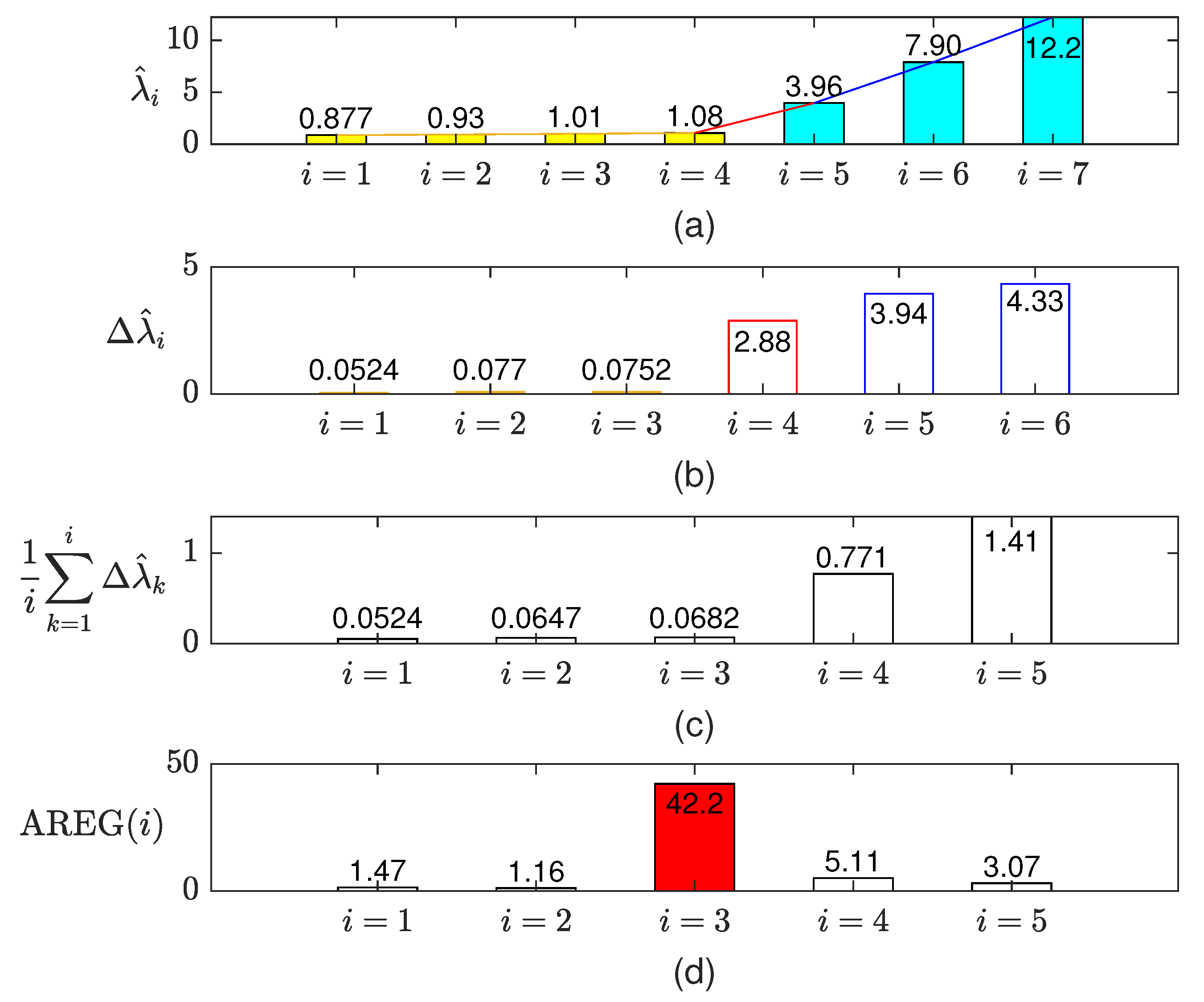
As mentioned in Section 4.1, AREG detects the NS gap using the ratio of the NS gap to the NN gap. In order to verify the performance of AREG, the eigenvalues, the gaps of eigenvalues, and the values of AREG are numerically analyzed. The parameters are set to M = 7 , ξ = η / 2 , D = 3 , θ 1 = 30 , θ 2 = 45 , θ 3 = 60 , AWGN with σ N 2 = 1 , SNR = 0 dB , and L = 1000 . Under these settings, R ^ x x is generated, and the eigenvalues are calculated.
Figure 2 shows the results of numerical analysis of AREG. Panel (a) shows the eigenvalues, where λ ^ 1 to λ ^ 4 denote the noise–subspace eigenvalues and λ ^ 5 to λ ^ 7 denote the signal–subspace eigenvalues. Because of σ N 2 = 1 , the values of noise–subspace eigenvalues are close to 1, while the values of signal–subspace eigenvalues are comparatively greater than 1.
Panel (b) shows the gaps of eigenvalues, where Δ λ ^ 1 to Δ λ ^ 3 denote NN gaps, Δ λ ^ 4 denotes the NS gap, and Δ λ ^ 5 and Δ λ ^ 6 denote SS gaps. This result shows that the NN gaps are comparatively smaller than the NS gap is; however, the greatest value is Δ λ ^ 6 , which is the SS gap. This is why the ratio of the NS gap to the NN gap is used in AREG to avoid wrong estimation which can be caused by using the greatest gap of eigenvalues for source enumeration.
Panel (c) shows the means of the accumulated gaps of eigenvalues, i.e., 1 i k = 1 i Δ λ k from (14). The means of the NN gaps (when i is 1, 2 and 3) are relatively small, while the mean of the NN gaps and the NS gap (when i is 4) and the mean of the NN gaps, the NS gap, and the SS gap (when i is 5) are comparatively greater than the means of the NN gaps are; this reduces the value of AREG even if the greatest gap is the SS gap because the denominator of AREG is increased when the NS gap or SS gap are included. As a result, the wrong estimation of the NS gap can be prevented.
Panel (d) shows the values of AREG. The result shows that AREG(3) is significantly greater than the other values of AREG—about eight times greater than AREG(4). According to (17), the estimated number of sources D ^ is 3; this result shows that AREG can estimate the right number of sources in an 0 dB SNR condition. In addition, under the same condition, 10,000 cases of AWGN are randomly generated, and the performances of AREG and AIC are compared. The result is that AREG estimates the number of sources in 100% accuracy while AIC has 90.03% accuracy.

5.2. Analysis of T-GANE

In this subsection, how to generate the datasets is firstly presented. Next, the values of BIC used for determining the number of GMM components and the estimated PDFs derived from the datasets are described. Finally, the probabilities and the optimal threshold, i.e., P MS , P FA , P Err , and γ ^ mentioned in (31)–(34) are shown.
In order to generate the datasets ( E NN data and E NS data ), the parameters—especially the range of arrival angle of signals ( θ min and θ max ) and the minimum angle difference between two adjacent signals ( Δ θ a b ) as shown in Figure 3—should be set; Δ θ a b is defined as
Δ θ a b = | θ a θ b | ( a b ) .
From our experiences, the NS gap is extremely small even at a high SNR when the arrival angle of a signal is too oblique (e.g., 80 or 80 ) or when the angle difference between two adjacent signals is small (e.g., 5 for Δ θ a b ). Generally, source enumeration and DOA estimation suffer from these extremely oblique impinging on ULA or high-resolution problems; but these problems are out of scope for this study, and those special situations probably degrade the learning performance of T-GANE because they will be outliers of the datasets. Therefore, the values of θ min , θ max and Δ θ a b should be limited when the datasets are generated. The parameters are set as follows:
Parameter Settings for Generation the Datasets
  • Number of elements of ULA M is 7.
  • Distance of the two adjacent elements ξ is η / 2 .
  • Number of signal sources D ranges from 1 to 6 (uniform random).
  • Arrival angle of signals θ i ( i = 1 , , D ) ranges from θ min = 60 to θ max = 60 (uniform random, non-discrete).
  • Minimum angle difference between the two adjacent signals Δ θ a b 15 .
  • Number of snapshots L is 1000.
  • SNR ranges from 20 dB to 10 dB (uniform random, non-discrete).
  • Number of situations for generating the datasets Q is 100,000.
Each situation, number of signal sources D, arrival angle of signals θ i ( i = 1 , , D ), and SNR are randomly selected subject to the parameter settings. From this simulation, 252,249 NN gaps and 100,000 NS gaps data are obtained.
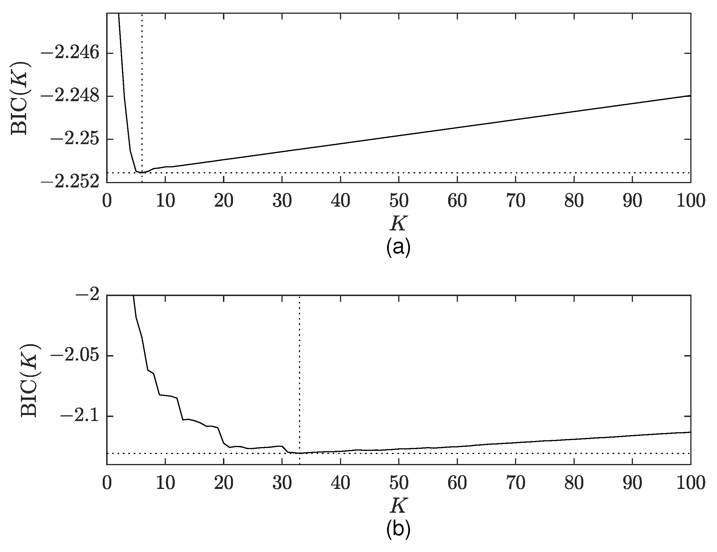
After generating E NN data and E NS data according to the parameter settings, Algorithm 1 with K max = 100 is executed to obtain the GMM parameters. Figure 4 shows the values of BIC versus the number of GMM components K; Panels (a) and (b) of Figure 4 show the results for E NN data and E NS data , respectively. Both results show that the value of BIC rapidly decreases for small K, then gradually increases for large K. Although there are some fluctuations of the BIC values in the results of panel (b), the smallest BIC values can be found; 6 for E NN data and 33 for E NS data .
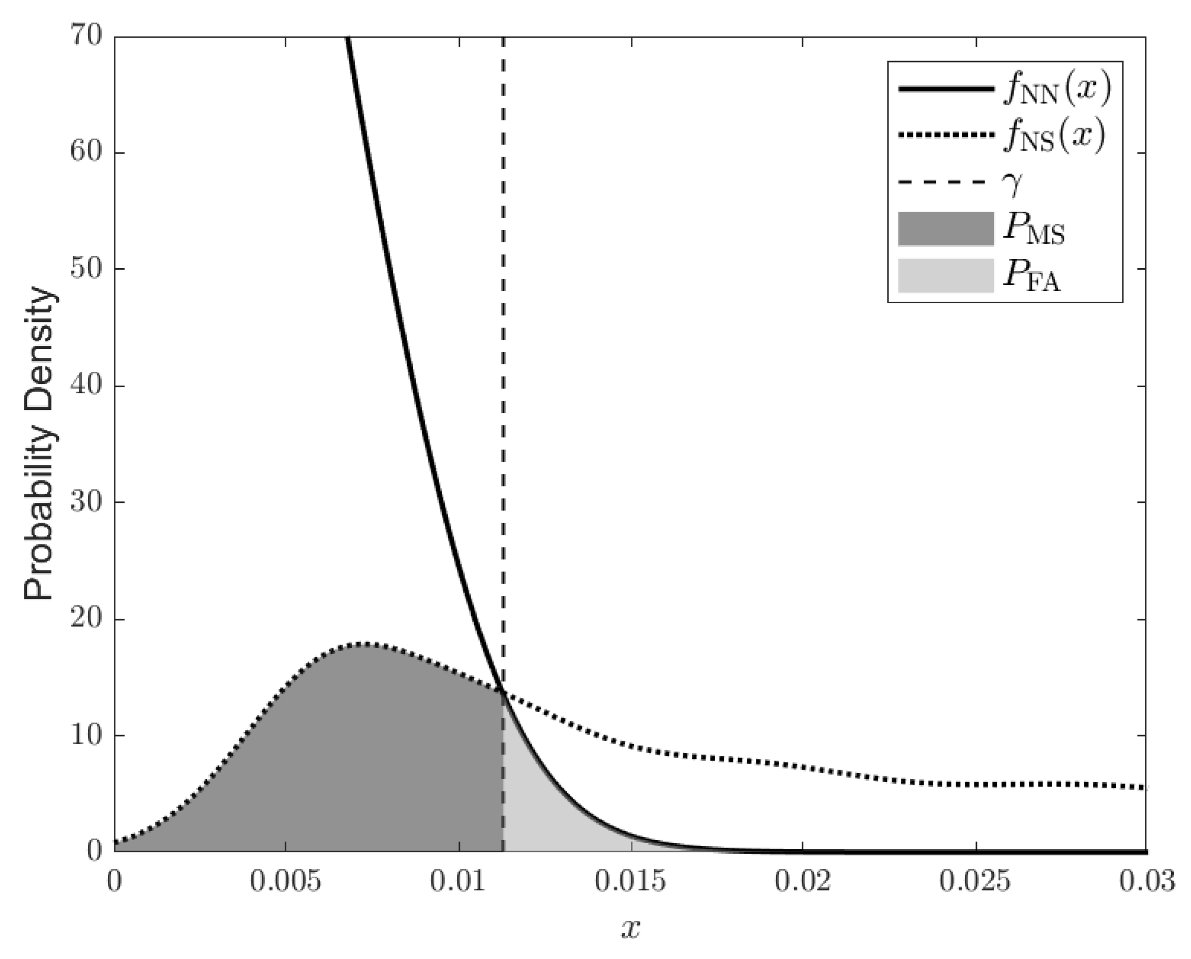
Figure 5 shows f NN ( x ) and f NS ( x ) obtained by Algorithm 1. Additionally, the visualization of (31) and (32) is also shown in Figure 5. As mentioned in Section 4.2.2, if a gap value is smaller than or equal to the threshold, then the gap is decided as the NN gap; the left-side of f NS ( x ) is mistaken for NN gaps. Otherwise, if a gap value is greater than the threshold, then the gap is decided as an NS gap; the right side of f NN ( x ) is mistaken for NS gaps.
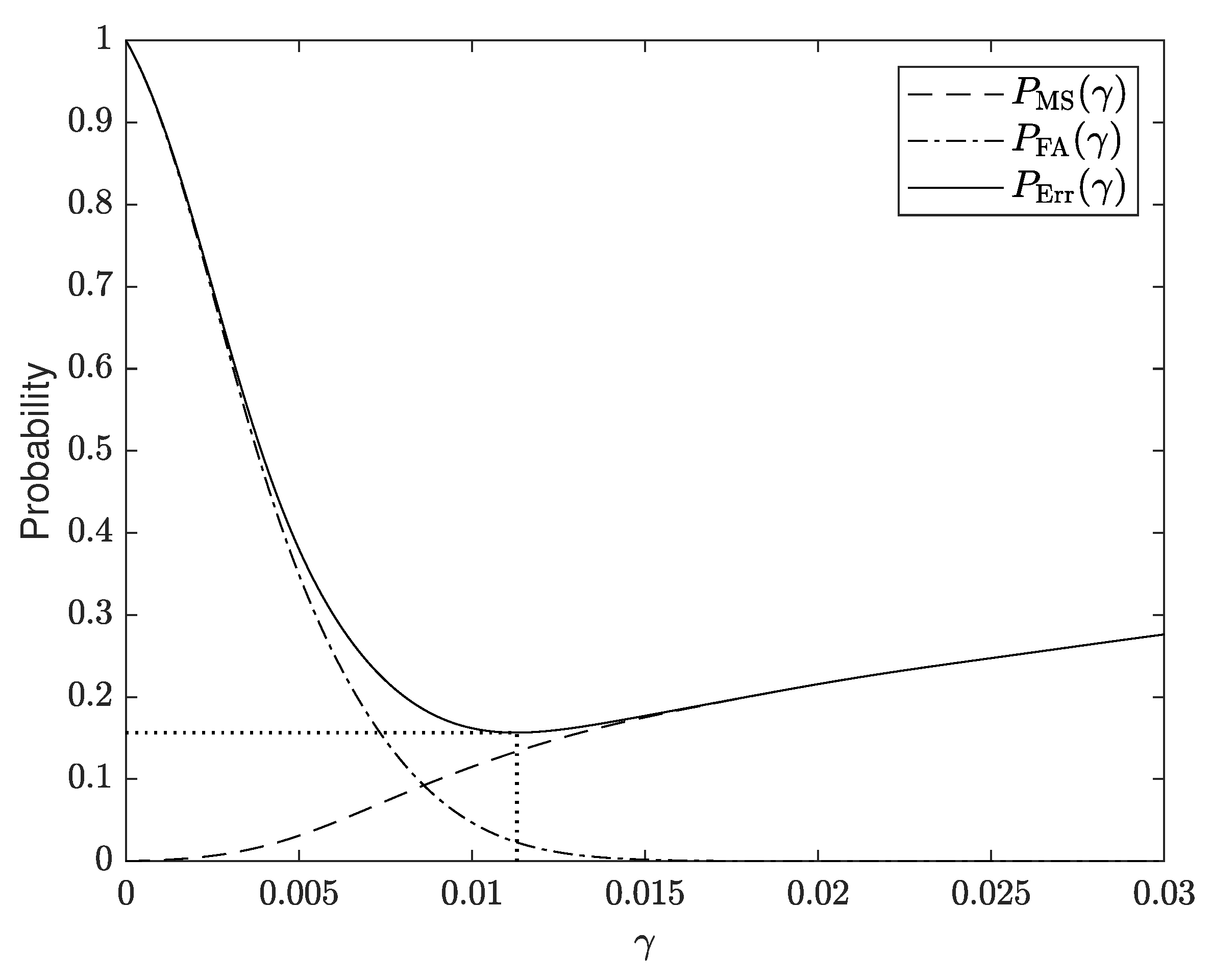
Figure 6 shows P MS ( γ ) , P FA ( γ ) , P Err ( γ ) , and the optimal threshold γ ^ that minimizes P Err . As shown in Figure 6, P MS ( γ ) is monotonically increasing, while P FA ( γ ) is monotonically decreasing. The graph of P Err ( γ ) shows that the minimum value of P Err ( γ ) is about 0.157 at γ = 0.0113 . Therefore, from (34), the optimal threshold γ ^ is set to 0.0113. The source enumeration performance with this optimal threshold will be shown in the next subsection.

5.3. Evaluation of Comprehensive Approaches

The performances of comprehensive approaches—AIC, MDL, SORTE, and our two proposed approaches (AREG and T-GANE)—are evaluated. First, the estimation accuracy of the approaches in various SNR conditions is described. Second, how many snapshots and ULA elements are required to provide 70% accuracy in various SNR conditions is presented. Finally, it is shown that T-GANE has the feasibility of improvement in low SNR performance with the designated SNR range for the generation of the datasets. The formulas of AIC and MDL refer to [12], and that of SORTE refers to [15], respectively. Our evaluation parameter settings are as follows:
Evaluation Parameter Settings
  • Number of elements of ULA M is 7.
  • Distance of the two adjacent elements ξ is η / 2 .
  • Number of signal sources D ranges from 1 to 4 (uniform random).
  • Arrival angle of signals θ i ( i = 1 , , D ) ranges from θ min = 60 to θ max = 60 (uniform random, non-discrete).
  • Minimum angle difference between the two adjacent signals Δ θ a b 15 .
  • Number of snapshots L is 1000.
  • Number of trials for each SNR is 10,000 times.
  • T-GANE is trained the same as is mentioned in Section 5.2.
Because the numerical detectability extent of SORTE is M 3 , the maximum D is set to 4. Note that γ ^ of T-GANE is set to 0.0113, and the source enumeration procedure of T-GANE is performed with Algorithm 2.
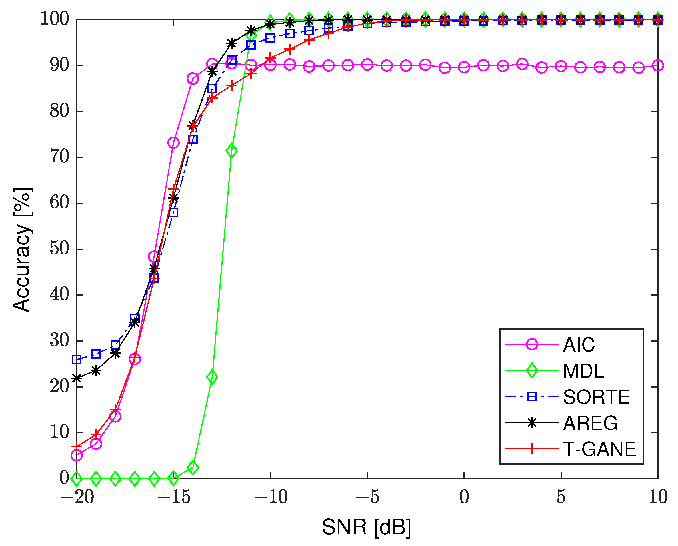
Figure 7 shows the estimation accuracy of AIC, MDL, SORTE, and our two proposed approaches (AREG, T-GANE) versus SNR. The performances are evaluated in the SNR range from 20 dB to 10 dB, which is roughly chosen in many other papers [4,10,11,12,14,16,23,24,25,31]. This paper is interested in improving accuracy of AIC at high SNR—where MDL has 100% accuracy, but AIC does not reach 100% accuracy—and it of MDL at low SNR—where the MDL accuracy begins to decrease sharply, but AIC maintais good accuracy. The results show that MDL, SORTE, AREG, and T-GANE have 100% accuracy at high SNR (roughly above 5 dB at this result), while AIC has about 90% accuracy despite a high SNR; however, AIC keeps its performance at about 13 dB and shows the best performance in SNR 15 dB to 13 dB among the approaches. SORTE and T-GANE begin to decrease below 5 dB, while AREG maintains 100% accuracy the same as MDL does. In the SNR range 14 dB to 5 dB, among AREG, SORTE, and T-GANE, AREG shows the best performance, the next is SORTE, and the third is T-GANE and its performance gradually decreases at that range of SNR. It is worth mentioning that the learning datasets certainly affect the performance of T-GANE; hence, T-GANE with another datasets is also evaluated, and the results are described afterwards.
Figure 8 shows the required number of snapshots (L) to provide 70% accuracy versus SNR. Note that the learning data for T-GANE are newly generated when the number of snapshots is changed (among the parameters, only the number of snapshots is changed; other parameters are not changed) and then the optimal thresholds are updated. Regardless of the approaches, the required number of snapshots sharply increases when SNR decreases. At the same SNR, AIC requires the smallest number of snapshots, while MDL requires the largest number of snapshots. SORTE, AREG, and T-GANE have similar performances, but our two proposed approaches have better performances than SORTE has. At the small number of snapshots (1000 to 5000), T-GANE has slightly better performance than AREG, while, for the large number of snapshots (6000 to 8000), AREG has slightly better performance than T-GANE. Over 8000 snapshots, the performance improvement of T-GANE is not as good as the other approaches. The reason is considered that the designated SNR range for generating datasets is fixed to 20 dB to 10 dB; if the designated SNR range for generating datasets is flexibly adjusted when the number of snapshots is changed, T-GANE may have better performance than that shown in Figure 8.
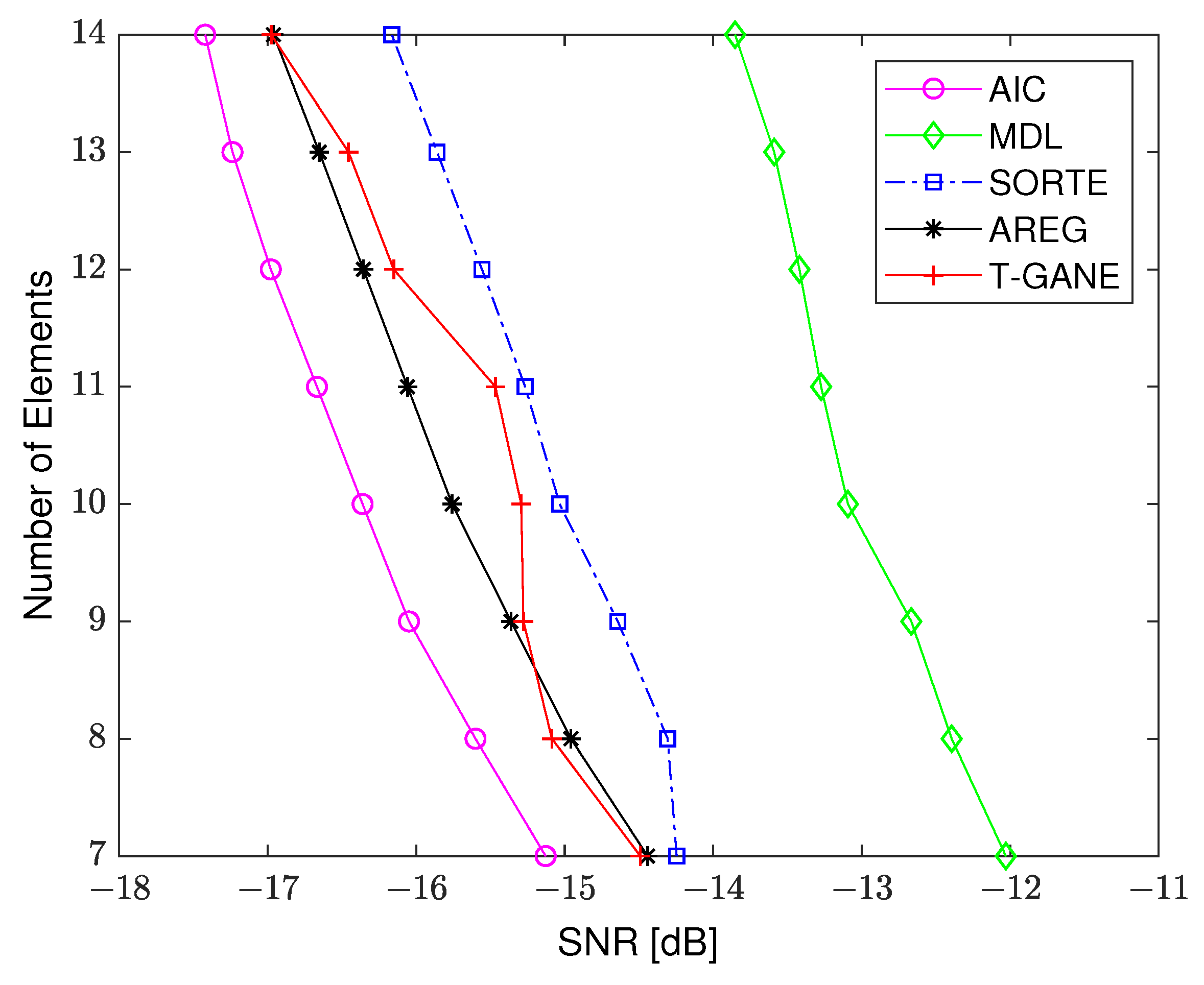
Figure 9 shows the required number of ULA elements (M) to provide 70% accuracy versus SNR. Note that the learning data for T-GANE are newly generated when the number of ULA elements is changed (among the parameters, only the number of ULA elements is changed; other parameters are not changed) and then the optimal thresholds are updated. Similar to the results of Figure 8, the required number of ULA elements sharply increases when SNR decreases regardless of the approaches. Our two proposed approaches have better performance than MDL and SORTE. Although T-GANE has unstable performance improvement compared to the others, it is expected that T-GANE can have stable performance improvement if appropriate datasets are provided for T-GANE as mentioned earlier.
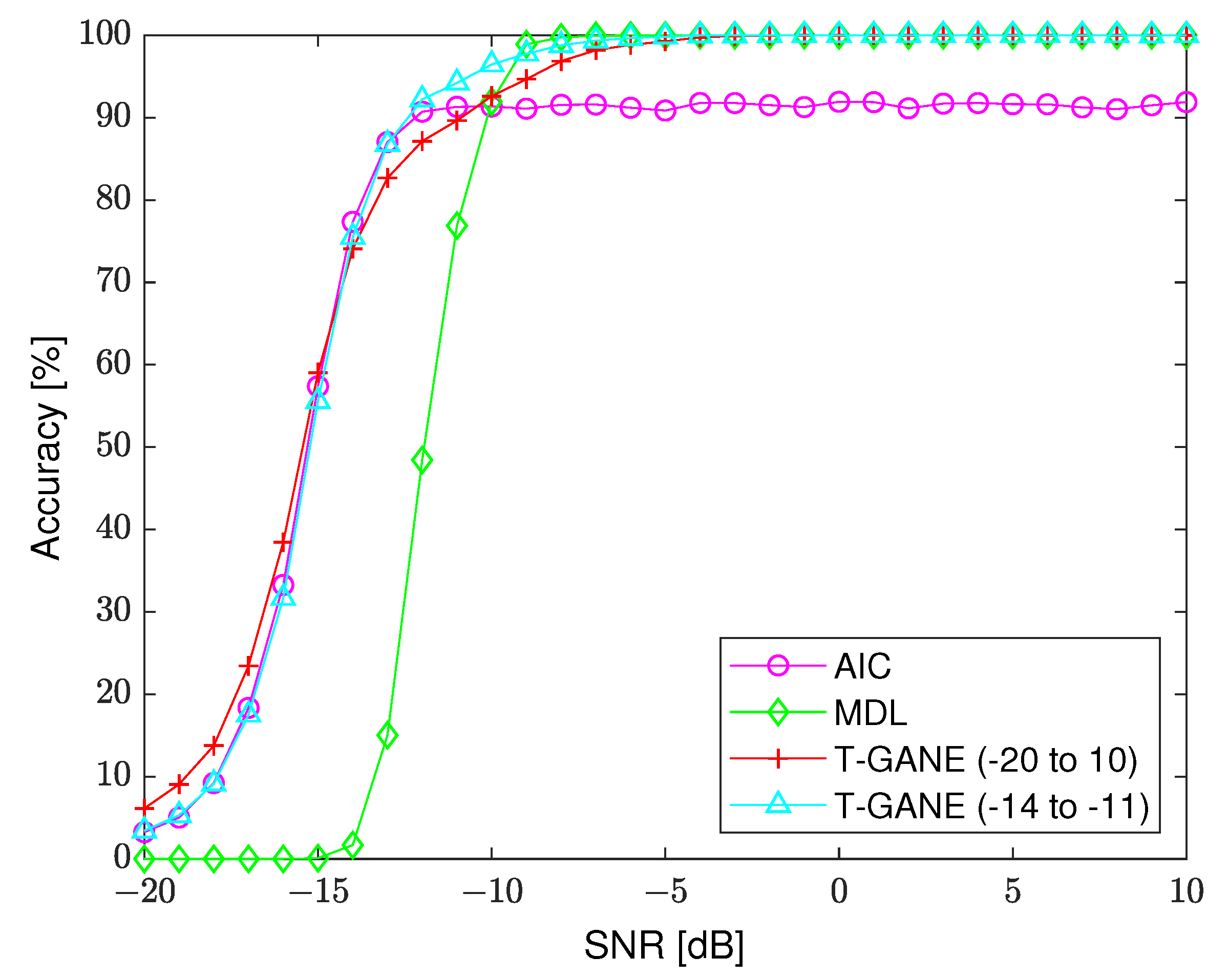
Figure 10 shows the estimation accuracy of AIC, MDL, T-GANE ( 20 to 10), and T-GANE ( 14 to 11 ), where T-GANE ( 20 to 10) and T-GANE ( 14 to 11 ) denote that the learning datasets for T-GANE are generated with the SNR range from 20 dB to 10 dB and from 14 dB to 11 dB, respectively. The reason why the learning datasets SNR is set to range from 14 dB to 11 dB is to improve the performance of T-GANE in the range of 14 dB to 11 dB, where the performances of AIC and MDL in Figure 7 begin to sharply decrease, respectively. Note that γ ^ of T-GANE ( 20 to 10) is 0.0113 and γ ^ of T-GANE ( 14 to 11 ) is 0.0125. In this evaluation, the number of signal sources D is randomly selected from a set { 1 , 2 , , 6 } at each trial; hence, SORTE and AREG are excluded from this evaluation. As shown in Figure 10, the estimation accuracy of T-GANE ( 14 to 11 ) is higher than T-GANE ( 20 to 10) for SNR over 14 dB (maximum 5.06% higher at SNR 12 dB). In addition, T-GANE ( 14 to 11 ) shows the best performance that surpasses AIC and MDL. From the results, it can be concluded that T-GANE has the feasibility of improvement performance at low SNR (roughly from 15 dB to 10 dB at this result) if appropriate learning datasets are used for T-GANE.
Although the learning SNR range of T-GANE ( 14 to 11 ) is less than that of T-GANE ( 20 to 10), T-GANE ( 14 to 11 ) has better performance for both low and high SNR than T-GANE ( 20 to 10). Typically, the NS gap is greater than NN gaps when the SNR is not too low. The difference between NS gap and NN gap is larger when the SNR is higher. If the slight difference between NS gap and NN gaps can be detected in a low SNR range, it is easy to detect the difference between them in a high SNR range; this is why T-GANE ( 14 to 11 ) also has good performance at high SNR. Meanwhile, if T-GANE learns too much high SNR information, it may be not easy to detect the slight difference between the NS gap and NN gaps because the difference between them is larger when the SNR is higher; this is why T-GANE ( 20 to 10) has worse performance than T-GANE ( 14 to 11 ). Intuitively, if the learning SNR range is too high level like from 0 dB to 10 dB, it probably has worse performance than T-GANE ( 20 to 10) at low SNR. Therefore, how to select the learning SNR range for T-GANE provides a good starting point for discussion and further research work.

6. Conclusions

In this paper, two source enumeration approaches named AREG and T-GANE are proposed. Both approaches employ gaps of eigenvalues from the covariance matrix of the received signals along multiple antenna arrays; AREG uses the ratio of the NS gap to the mean of accumulated NN gaps, while T-GANE uses the gaps of the normalized eigenvalues to compute the threshold by machine learning based clustering approaches. The criterion formula of AREG using the gaps of eigenvalues is derived, and a source enumeration criterion with AREG is presented. Three steps of the T-GANE procedure are also described: dataset generation, learning and computing optimal threshold, and source enumeration using the optimal threshold. The simulation results show that AREG provides better accuracy of source enumeration than that of MDL and SORTE at a low SNR range and is also better than that of AIC at high SNR. It is also shown that T-GANE with appropriate learning datasets outperforms both AIC and MDL in high and low SNR. This feasibility shows that the appropriate parameter settings for generating learning datasets of T-GANE in the designated SNR range are sought to improve the T-GANE as future research work.

Author Contributions

Conceptualization, Y.L., C.P., Y.C., and K.K.; methodology, Y.L. and C.P.; software, Y.L., C.P., and T.K.; validation, Y.L. and C.P.; formal analysis, Y.L. and C.P.; investigation, Y.L., C.P., and T.K.; resources, Y.C. and K.K.; data curation, Y.L., D.K., M.-S.L., and D.L.; writing—original draft preparation, Y.L., C.P., and T.K.; writing—review and editing, Y.L., Y.C., and K.K.; visualization, Y.L., C.P., and T.K.; supervision, Y.C., K.K., D.K., M.-S.L., and D.L.; project administration, Y.C., K.K., D.K., M.-S.L., and D.L.; funding acquisition, Y.C., K.K., D.K., M.-S.L., and D.L. All authors have read and agreed to the published version of the manuscript.

Funding

This work was supported by the Agency for Defense Development, Republic of Korea, under the contract “V/UHF Communication Electronic Support System of Electronic Warfare UAV”.

Institutional Review Board Statement

Not applicable.

Informed Consent Statement

Not applicable.

Data Availability Statement

Not applicable.

Conflicts of Interest

The authors declare no conflict of interest.

References

  1. Choi, S.; Kwon, O.-J.; Oh, H.; Shin, D. Method for Effectiveness Assessment of Electronic Warfare Systems in Cyberspace. Symmetry 2020, 12, 2107. [Google Scholar] [CrossRef]
  2. Adamy, D. EW 101: A First Course in Electronic Warfare; Artech House: Norwood, MA, USA, 2001; ISBN 1580531695. [Google Scholar]
  3. Liu, M.; Zhang, J.; Tang, J.; Jiang, F.; Liu, P.; Gong, F.; Zhao, N. 2D DOA robust estimation of echo signals based on multiple satellites passive radar in the presence of alpha stable distribution noise. IEEE Access 2019, 7, 16032–16042. [Google Scholar] [CrossRef]
  4. Pan, Q.; Mei, C.; Tian, N.; Ling, B.W.-K.; Wang, E.X.; Yang, Z. An effective sources enumeration approach for single channel signal at low SNR. IEEE Access 2019, 7, 31055–31067. [Google Scholar] [CrossRef]
  5. Schmidt, R. Multiple emitter location and signal parameter estimation. IEEE Trans. Antennas Propag. 1986, 34, 276–280. [Google Scholar] [CrossRef] [Green Version]
  6. Roy, R.; Kailath, T. ESPRIT-estimation of signal parameters via rotational invariance techniques. IEEE Trans. Acoust. 1989, 37, 984–995. [Google Scholar] [CrossRef] [Green Version]
  7. Yan, F.-G.; Wang, J.; Liu, S.; Cao, B.; Jin, M. Computationally efficient direction of arrival estimation with unknown number of signals. Digit. Signal Process. 2018, 78, 175–184. [Google Scholar] [CrossRef]
  8. Baral, A.B.; Torlak, M. Impact of number of noise eigenvectors used on the resolution probability of MUSIC. IEEE Access 2019, 7, 20023–20039. [Google Scholar] [CrossRef]
  9. Yan, F.-G.; Cao, B.; Liu, S.; Jin, M.; Shen, Y. Reduced-complexity direction of arrival estimation with centro-symmetrical arrays and its performance analysis. Signal Process. 2018, 142, 388–397. [Google Scholar] [CrossRef]
  10. Xu, K.; Pedrycz, W.; Li, Z.; Nie, W. High-accuracy signal subspace separation algorithm based on Gaussian kernel soft partition. IEEE Trans. Ind. Electron. 2019, 66, 491–499. [Google Scholar] [CrossRef]
  11. Pan, Q.; Mei, C.; Tian, N.; Ling, B.W.-K.; Wang, E.X. Source enumeration based on a uniform circular array in a determined case. IEEE Trans. Veh. Technol. 2019, 68, 700–712. [Google Scholar] [CrossRef]
  12. Wax, M.; Kailath, T. Detection of signals by information theoretic criteria. IEEE Trans. Acoust. 1985, 33, 387–392. [Google Scholar] [CrossRef] [Green Version]
  13. Van Trees, H.L. Optimum Array Processing; John Wiley & Sons, Inc.: New York, NY, USA, 2002; ISBN 0471093904. [Google Scholar]
  14. Badawy, A.; Salman, T.; Elfouly, T.; Khattab, T.; Mohamed, A.; Guizani, M. Estimating the number of sources in white Gaussian noise: Simple eigenvalues based approaches. IET Signal Process. 2017, 11, 663–673. [Google Scholar] [CrossRef]
  15. He, Z.; Cichocki, A.; Xie, S.; Choi, K. Detecting the number of clusters in n-way probabilistic clustering. IEEE Trans. Pattern Anal. Mach. Intell. 2010, 32, 2006–2021. [Google Scholar] [CrossRef]
  16. Wu, X.; Zhu, W.-P.; Yan, J. A fast gridless covariance matrix reconstruction method for one- and two-dimensional direction-of-arrival estimation. IEEE Sens. J. 2017, 17, 4916–4927. [Google Scholar] [CrossRef]
  17. Zuo, W.; Xin, J.; Zheng, N.; Sano, A. Subspace-based localization of far-field and near-field signals without eigendecomposition. IEEE Trans. Signal Process. 2018, 66, 4461–4476. [Google Scholar] [CrossRef]
  18. Lonkeng, A.D.; Zhuang, J. Two-dimensional DOA estimation using arbitrary arrays for massive MIMO systems. Int. J. Antennas Propag. 2017, 2017, 1–9. [Google Scholar] [CrossRef]
  19. Nie, W.; Xu, K.; Feng, D.; Wu, C.; Hou, A.; Yin, X. A fast algorithm for 2D DOA estimation using an omnidirectional sensor array. Sensors 2017, 17, 515. [Google Scholar] [CrossRef] [PubMed] [Green Version]
  20. Yan, F.-G.; Yan, X.-W.; Shi, J.; Wang, J.; Liu, S.; Jin, M.; Shen, Y. MUSIC-like direction of arrival estimation based on virtual array transformation. Signal Process. 2017, 139, 156–164. [Google Scholar] [CrossRef]
  21. Weng, Z.; Djurić, P.M. A search-free DOA estimation algorithm for coprime arrays. Signal Process. 2014, 24, 27–33. [Google Scholar] [CrossRef] [Green Version]
  22. Cho, C.-M.; Djuric, P.M. Detection and estimation of DOA’s of signals via Bayesian predictive densities. IEEE Trans. Signal Process. 1994, 42, 3051–3060. [Google Scholar] [CrossRef] [Green Version]
  23. Han, K.; Nehorai, A. Improved source number detection and direction estimation with nested arrays and ULAs using jackknifing. IEEE Trans. Signal Process. 2013, 61, 6118–6128. [Google Scholar] [CrossRef]
  24. Chen, W.; Wong, K.M.; Reilly, J.P. Detection of the number of signals: A predicted eigenthreshold approach. IEEE Trans. Signal Process. 1991, 39, 1088–1098. [Google Scholar] [CrossRef]
  25. Hu, O.; Zheng, F.; Faulkner, M. Detecting the number of signals using antenna array: A single threshold solution. In Proceedings of the Fifth International Symposium on Signal Processing and its Applications (ISSPA ’99), Brisbane, QLD, Australia, 22–25 August 1999; pp. 905–908. [Google Scholar] [CrossRef]
  26. Bkassiny, M.; Li, Y.; Jayaweera, S.K. A survey on machine-learning techniques in cognitive radios. IEEE Commun. Surv. Tutor. 2013, 15, 1136–1159. [Google Scholar] [CrossRef]
  27. Stanković, Z.; Dončov, N.; Milovanović, I.; Milovanović, B. Direction of arrival estimation of mobile stochastic electromagnetic sources with variable radiation powers using hierarchical neural model. Int. J. RF Microw. Comput. Eng. 2019, 29, e21901. [Google Scholar] [CrossRef]
  28. Liu, Z.-M.; Zhang, C.; Yu, P.S. Direction-of-arrival estimation based on deep neural networks with robustness to array imperfections. IEEE Trans. Antennas Propag. 2018, 66, 7315–7327. [Google Scholar] [CrossRef]
  29. Huang, H.; Yang, J.; Huang, H.; Song, Y.; Gui, G. Deep learning for super-resolution channel estimation and DOA estimation based massive MIMO system. IEEE Trans. Veh. Technol. 2018, 67, 8549–8560. [Google Scholar] [CrossRef]
  30. Yang, Y.; Gao, F.; Qian, C.; Liao, G. Model-aided deep neural network for source number detection. IEEE Signal Process. Lett. 2020, 27, 91–95. [Google Scholar] [CrossRef] [Green Version]
  31. Yun, W.; Xiukun, L.; Zhimin, C.; Jian, H.; Haiwei, M.; Zhentao, W. Joint signal-to-noise ratio and source number estimation based on hierarchical artificial intelligence units. Meas. Sci. Technol. 2018, 29, 095104. [Google Scholar] [CrossRef]
  32. Hamid, M.; Bjorsell, N.; Ben Slimane, S. Sample covariance matrix eigenvalues based blind SNR estimation. In Proceedings of the 2014 IEEE International Instrumentation and Measurement Technology Conference (I2MTC), Montevideo, Uruguay, 12–15 May 2014; pp. 718–722. [Google Scholar] [CrossRef]
  33. Ganjavi, A.; Christopher, E.; Johnson, C.M.; Clare, J. A study on probability of distribution loads based on expectation maximization algorithm. In Proceedings of the 2017 IEEE Power & Energy Society Innovative Smart Grid Technologies Conference (ISGT), Washington, DC, USA, 23–26 April 2017. [Google Scholar] [CrossRef]
  34. McLachlan, G.J.; Peel, D. Finite Mixture Models; John Wiley & Sons, Inc.: New York, NY, USA, 2000; ISBN 0471006262. [Google Scholar]
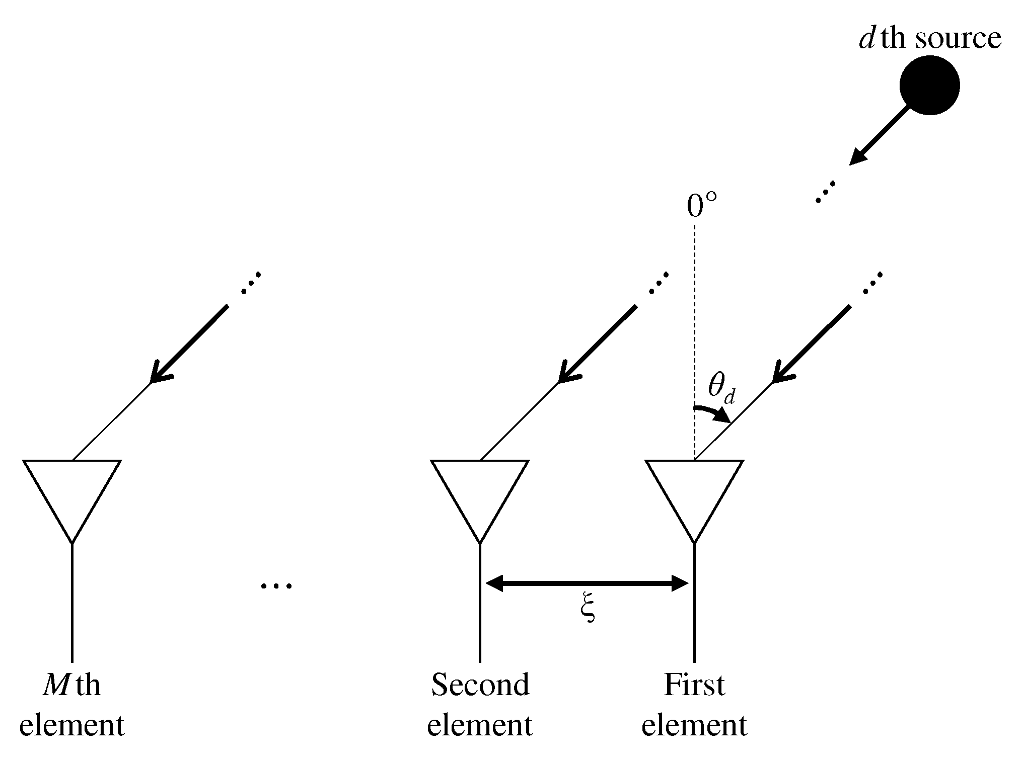
Figure 1. Our considered ULA model.
Applsci 11 01942 g001
Figure 2. Numerical analysis of AREG. (a) the eigenvalues; (b) the gaps of eigenvalues; (c) the means of the accumulated gaps of eigenvalues; (d) the values of AREG.
Applsci 11 01942 g002
Figure 3. The range of arrival angle of signals and the angle difference between the two adjacent signals.
Applsci 11 01942 g003
Figure 4. Values of BIC versus the number of GMM components. (a) the BIC values for E NN data ; (b) the BIC values for E NS data .
Applsci 11 01942 g004
Figure 5. PDFs f NN ( x ) and f NS ( x ) . Probabilities P MS ( γ ) and P FA ( γ ) are also visualized.
Applsci 11 01942 g005
Figure 6. P MS ( γ ) , P FA ( γ ) , P Err ( γ ) and the optimal threshold γ ^ that minimizes P Err .
Applsci 11 01942 g006
Figure 7. Estimation accuracy of AIC, MDL, SORTE, and our two proposed approaches (AREG, T-GANE) versus SNR. The number of signal sources D is randomly selected from a set { 1 , 2 , 3 , 4 } at each trial.
Applsci 11 01942 g007
Figure 8. Required number of snapshots (L) to provide 70% accuracy versus SNR. The number of signal sources D is randomly selected from a set { 1 , 2 , 3 , 4 } at each trial.
Applsci 11 01942 g008
Figure 9. Required number of ULA elements (M) to provide 70% accuracy versus SNR. The number of signal sources D is randomly selected from a set { 1 , 2 , 3 , 4 } at each trial.
Applsci 11 01942 g009
Figure 10. The estimation accuracy of AIC, MDL, and T-GANE versus SNR. T-GANE ( 20 to 10) and T-GANE ( 14 to 11 ) denote that the learning datasets for T-GANE are generated for SNR range 20 dB to 10 dB and 14 dB to 11 dB, respectively. The number of signal sources D is randomly selected from a set { 1 , 2 , , 6 } at each trial.
Applsci 11 01942 g010
Publisher’s Note: MDPI stays neutral with regard to jurisdictional claims in published maps and institutional affiliations.