Model-Based Dynamic Forecasting for Residential Construction Market Demand: A Systemic Approach

Abstract

According to the previous research, proper demand forecasting could help construction-related firms in effective planning for future market changes. However, existing market demand forecasting models are somewhat limited, and most of them bear some critical shortcomings. This research aims to develop a forecasting model for the Korean residential construction industry using system dynamics. In developing the market forecasting model, this research uses variables that significantly impact future construction market change. Many of the existing models do not include as many variables as this model, and none of them have considered complex interlocking effects among these variables. This model is also the first model using a system-based approach by looking at the target industry as a ‘one complex system’ rather than focusing on individual variables’ impact on future market changes. By employing system dynamics, it is possible to consider qualitative and quantitative aspects and produce long-term market forecasting results. The developed market forecasting model consists of two main modules, the first being a prediction module for the grassroots construction market and the second for operation and maintenance (O&M) and the demolition market. Sixteen input variables are grouped into four categories: social, economy, regulation, and past market size among over 25 identified variables. The model utilizes a mathematical function system using the designed feedback loops in producing future market forecasts. Based on the validation tests with past market data, it turns out that the model is reliable, with the determination coefficient (R²) being over 0.7 on all tested occasions. According to the model’s forecasting results, the Korean construction market’s size is expected to be 231 billion won in 2015 and 286 billion won in 2030. However, the O&M market’s growth rate is expected to be higher than 180%, which is much bigger than those of the grass-root and demolition markets. Thus, this research model is realistic according to the construction paradigm change. This research is considered one of the pioneering studies in construction market forecasting by employing dynamic inter-relationships among various input variables. Therefore, the market forecasting results can be interpreted as more practical and can provide more insights to the construction industry stakeholders. The model is envisioned to provide the public sector with useful guidelines in preparing future public market supply strategies such as construction budget allocations. It would also be helpful for the private sector to develop more proactive and accurate demand strategies for timely decision-making.

1. Introduction

1.1. Background and Research Objectives

The construction industry is an industry that has information asymmetry and transaction opacity. Since the construction industry mainly deals with closed offline transactions, access to information on companies and prices is very low. These problems cause a negative perception of society in the construction industry. The construction industry needs to change the demand structure by securing transactions’ accessibility and transparency by changing the offline-oriented market to online-centered like other industries, it is necessary to analyze the industry’s size, the existing demand environment, and future demand accurately to transform the demand structure.

Forecasting the size of demand is significant because it not only grasps market trends but also affects overall management activities [1]. Scientific forecasting considering market trends and environmental changes can increase market priorities and market competitiveness. The company’s supply strategies are also established based on the strategy and countermeasure analysis results through market demand forecast [2,3]. Since supply strategies originating from uncertain and unrealistic forecasting can lead to unnecessary waste of resources and lag in industrial competition, it is most important to minimize uncertainty in forecasting by applying appropriate forecasting techniques according to the forecasting’s purpose and environment [4]. Demand forecasting can promote the industry’s revitalization by creating a new business model for suppliers by establishing a proactive response strategy according to future demand changes.

Demand forecasting is imperative in the domestic construction industry due to the considerable variation in demand due to changes in the social, industrial, and technological environment [5]. The residential architecture market is expanding in line with the social atmosphere of stabilizing the real estate market by expanding supply. As the industry enters the maturity period of quantitative growth, the public infrastructure market centered on roads, dams, and tunnels is shrinking [6]. New markets are created around smart construction technologies in which new technologies such as artificial intelligence, big data, and clouding are integrated into the construction industry. Accurate forecasting of demand volatility and proactive response significantly impact the construction industry [7].

The construction market is an industry with dynamic changes that occur when internal and external environmental factors influence each other and need to grasp demand changes through a scientific and systemic approach from a macroscopic perspective for realistic demand forecasting [8,9]. This systemic approach enables forecasting the actual demand and diffusion trend of the construction market and market volatility and is considered a more effective forecasting method for market changes. Also, by providing a strategic basis for both consumers and suppliers based on objective data on the market’s ripple effect due to environmental changes, it is possible to provide future market preemption opportunities and increase corporate competitiveness by maximizing productivity. This study is based on the characteristics of complex structural changes in the construction market. The model focuses on the model’s usefulness and usability to develop a model that can identify how the dynamic relationship between the subsystems that make up the massive construction market system will change in the long term.

This study develops a model to forecast the size of demand in the construction market based on a systematic approach. The developed model’s primary utilization value is to analyze the existing demand environment and forecast the future demand scale. Changing the construction industry’s demand structure can provide a basis for structural change by accurately analyzing and predicting the demand scale.

1.2. Research Methods and Procedures

The content scope of this study is limited to the residential construction market. The construction industry’s market structure is primarily divided into the residential market, non-residential market, and infrastructure market, with each type having market-specific characteristics [10,11]. This study develops demand forecasting models, and forecasts demand, focusing on the residential market, where the share of the domestic construction market is rapidly increasing.

This study develops a model by applying qualitative and quantitative methods. The process of collecting and designing model data focuses on prior research and collecting expert opinions. A computer model based on computational mathematical structures is constructed through time-series data collection and analysis in the model development and simulation process.

This study establishes the rationale for system modeling using literature research and standardized data. The system dynamics research methodology is adopted as the core research methodology to implement and measure changes in the construction market that are close to reality. Powersim Studio 10 is used for model building and simulation analysis using the system dynamics methodology.

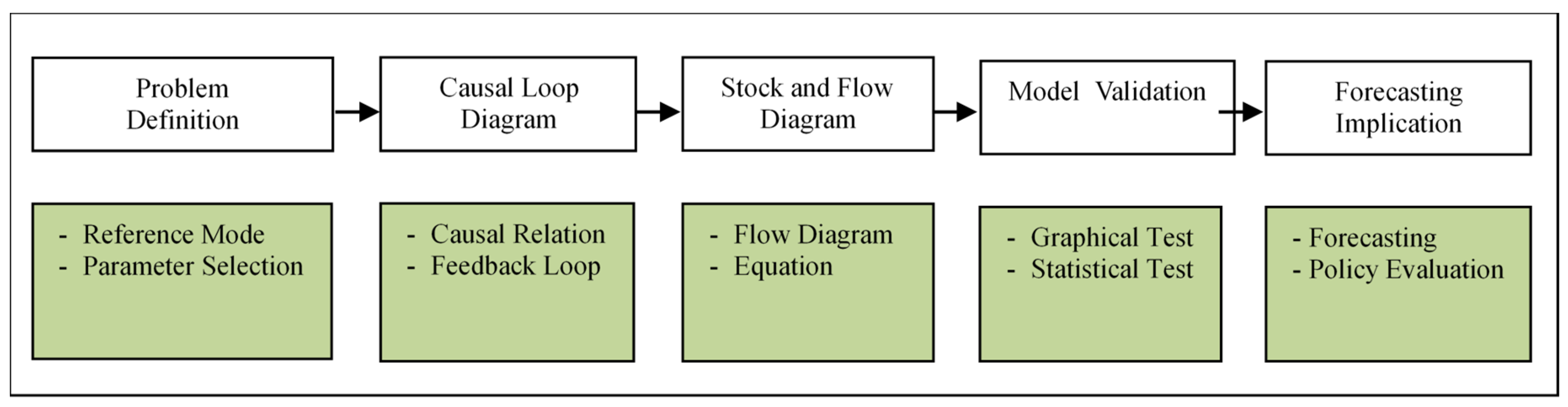
This study’s scope is based on the problem definition and secures the model’s validity through the model’s design, development, and verification process. Also, sensitivity analysis is performed to analyze the degree of impact of key variables on the system. Finally, through the simulation process, a range of construction market demand forecasting is generated according to the control variables’ management. Figure 1 summarizes research methods and procedures.

1.3. Research Methods and Procedures

Before conducting the research, a survey of prior studies on construction using system dynamics was conducted. Forrester used system dynamics in the urban dynamics model to describe the various interaction structures in US cities and attempted to model the residential sector as a sub-sector for the first time. The model consists of five subsystems: the industrial sector, the population sector, the residential sector, the tax sector, and the urban development sector, and the interaction between the subsystems is modeled as causing urban growth and policy decline [12,13]. The residential problem comprises many diverse and complex factors such as economics, society, culture, and politics, so the solution also has the characteristics of comprehensive measures covering tax financing, residential supply, and residential development. Thus, an understanding of complex residential market mechanisms and comprehensive analysis methods is required to evaluate residential policies. Also, there are bound to be limitations in explaining the impact of policies.

The primary domestic studies that applied system dynamics to the construction industry-related fields include Kim [14], Park et al. [15], Shin [16], Korea Research Institute for Human Settlements [10], and the Korea Institute of Science and Technology Evaluation and Planning [17] (

Table 1. Literature research of construction using system dynamics in Korea.

Research	Summary	Implications
Kim [14]	Write a simulation model that hinders the activation of the Construction Management (CM) market and suggest ways to improve each risk factor	Qualitative and quantitative analysis results
Park et al. [15]	Development of System Dynamics (SD) model based on primary factors that make up the residential market and the impact of the government’s deregulation on mortgage market participants	Qualitative analysis results
Shin [16]	Building an artificial residential market model by dividing the residential market into demand market, residential price, and supply market and identifying the causal relationship	Qualitative and quantitative analysis results Model verification and utilization results
Korea Research Institute for Human Settlements [20]	Development of traffic demand forecasting model and evaluation of predictive power for various development techniques including system dynamics model	Qualitative and quantitative analysis results Comparison of model development by research methods
An [21]	Establishing a construction cost estimation model based on the analysis of public residential project performance cost	Qualitative and quantitative analysis results
Korea Institute of S&T Evaluation and Planning [17]	Comparative model development and simulation results of government research and development (R&D) investment using system dynamics and artificial neural network	Qualitative and quantitative analysis results Model verification and utilization results Comparison of model development by research methods
Kang et al. [22]	Analysis of the mechanism of system operation based on the causal relationships between the variables in the real estate market	Qualitative analysis results

).

The main overseas studies that applied system dynamics to the construction industry-related fields include Park [18] and Onat et al. [19] (

Table 2. Literature research on construction using overseas system dynamics.

Research	Summary	Implications
Park [18]	Development of an analytical model for the effective management of physical and human resources	Qualitative and quantitative analysis results Model verification and utilization results Presenting model simulator
Zhou et al. [23]	Development of sustainability indicators for infrastructure projects using dynamic models	Qualitative and quantitative analysis results Model verification and utilization results
Shin et al. [24]	Development of a risk recognition model to understand the unsafe behavior of construction workers	Qualitative and quantitative analysis results Model verification and utilization results
Onat et al. [19]	Analysis of the effect of energy consumption on greenhouse gas emission in residential facilities	Qualitative and quantitative analysis results Model verification and utilization results Forecasting model results by scenarios

).

2. Overview on System Dynamics

2.1. Definition of System Dynamics

Industrial dynamics dealing with unstable changes in industrial inventory, labor force, and reduced occupancy rates was first published in 1961 by Professor Jay W. Forrester of Massachusetts Institute of Technology University in the US. It started by developing and applying a model to use in the US military’s production and inventory management, based on the thinking that the circular loop theory used in electrical engineering can be applied to general social systems [4,25].

Forrester described system dynamics as a methodology for estimating the pattern of growth or change by realistically depicting the interrelationships among the factors that cause changes in the system. Kim [26] defines system dynamics as a method to implement hypotheses conceivable in reality without any actual loss by logically reconstructing multi-layered and mutually complicated social variables and implementing them on a computer very similar to the real world. Kim [27] defined system dynamics as a methodology that analyzes policy effects by modeling a system’s structure and simulating it in a computer [28].

System dynamics is also useful as a methodology for observing the degree of influence between variables by looking at a system composed of variables related to a problem over time [29,30]. In the model reflecting social phenomena, the flow of problems through the feedback structure can be understood, and various changes can be analyzed through simulation. System dynamics defines a system composed of variables related to phenomena or problems and quantifies the relationships between the variables to model on the computer. System dynamics helps to explain and solve problems by revealing the dynamic characteristics of the system through simulation. It is a practical science that analyzes, applies, and predicts complex and changing social phenomena using computers.

2.2. Characteristics of System Dynamics

System dynamics has unique characteristics that distinguish it from other research methods. First, system dynamics does not differentiate between dependent and independent variables. System dynamics focuses on the mutual causal relationships between the variables—independent variables can be influenced by dependent variables and vice versa. Also, it excludes the independence between independent variables and assumes the mutual effect of the dependent variables. Second, system dynamics are based on a cyclical causal relationship, not a single causal relationship, and has a unique status compared to a conventional single-line and static research method as it facilitates dynamic analysis rather than static analysis [31]. Third, system dynamics finds the cause of the dynamic change in the feedback structure. The feedback structure means that a causal relationship between variables is interconnected to form a closed-circuit.

Thus, system dynamics has different approaches and analysis viewpoints, as shown in

Table 3. Comparison of prediction simulation types and features.

Type	Quantitative Analysis	System Dynamics Analysis
Inference method	Existing empirical data	Cause and effect relationship between variables
Analysis target	Static form	Dynamic form
Analysis focus	Correlation between two variables	Cyclical relation among multiple variables
Analysis goal	Numerical accuracy	Structural accuracy

, compared to the most commonly used statistical methods. This difference suggests that system dynamics and statistical improvement techniques are complementary rather than mutually competitive. In other words, for the same policy research project, it is possible to take advantage of both by simultaneously using system dynamics that emphasize the structure of the system and statistical metrics that emphasize the behavior of the system [31].

3. Results Concept of Construction Demand Forecasting Model

3.1. Definition of Construction Demand Forecasting Model

The construction demand forecasting model approaches the concept of asset value evaluation as a money-based approach rather than a quantity-based approach to grasp the number of facilities in estimating the future domestic construction market size [32,33]. To objectively verify the actual status of facilities when predicting the market size based on the number of facilities, it is not easy to quantitatively collect and pre-process the vast amount of performance data [34]. Also, there is a limitation that the quantity base cannot correctly evaluate the quality level over time, such as the social, economic, functional, and aging status of facilities [35]. However, there is an advantage that it is possible to evaluate the construction value based on the monetary value as an economic value [21]. For example, even if the same amount of road extension level exists, it is difficult to consider the actual performance due to different functions depending on the facility’s degree of aging [36]. However, it is possible to reflect aging considering the facility’s depreciation as a monetary value standard.

3.2. Structure of Construction Demand Forecasting Model

The construction demand forecasting model has a system structure system of the stock-flow diagram (Stock-Flow Diagram) and has two new construction demand forecasting module (Module I) and maintenance and demolition’s construction demand forecasting module (Module II). It occurs when modules are connected in sequence.

Module I is a module for estimating new construction demand generated by changes in the construction market’s external environment and is set based on the construction market size data from 2000 to 2015. Module I improves predictive reliability through a fitting process for optimal parameter estimation based on the amount of change in explanatory environmental variables such as various societies, economies, and institutions surrounding the domestic construction market. During this period, the construction demand forecast will be conducted from 2016 to 2030 after the significance test of the historical and predicted data on the new construction market’s size. Module II occurs through systemic linkage with Module I. It is set based on the construction capital stock, and the flow amount changes according to the degree of inflow–outflow. New construction demand for the year generated in Module I is converted into value as it flows into the construction capital stock and begins to accumulate with the inflow to the previous point. As the value decreases over time, it is converted into maintenance and demolition demand, and the value is decreased until the set service life of the original type is reached.

Maintenance demand forecasts are generated from accumulated construction capital stock. Depending on each asset’s useful life, the facility’s value regularly declines until the point of large-scale maintenance reinforcement [37,38]. The value calculated at this point is captured as demand for maintenance [39]. At this stage, correction is necessary to estimate realistic maintenance demand. The actual maintenance demand is estimated by revising the pattern coefficient to reflect the trend, such as the recent increase in the amount of maintenance and the conversion coefficient to apply the maintenance cost to the new construction cost by construction type. The demolition demand forecast sets when the facility’s function reaches zero, and each asset’s useful life requires the demolition plan. At this stage, the value generated is the demand for demolition. Estimates of demolition demand are predicted by correcting the recent demolition trends and application of maintenance rate to estimate final demolition demand.

The total construction demand forecast result is the sum of the new demand forecast calculated in Module I and the maintenance and demolition demand forecast in Module II. With the model design based on the integrated system, it is possible to calculate the demand forecasting results and the detailed step-by-step (new, maintenance, and demolition) forecasting results of the construction production process that occur continuously over time.

3.3. Identification of Parameters

In order to build a system dynamics model, appropriate configuration variables must be selected. If too many variables are included, the system structure is complicated, and it is difficult to understand the overall causal relationship between the variables. Also, if too few variables are included, it is difficult to find the problem’s cause.

It is difficult to find literature that introduces the scope setting for the size or number of related construction variables. However, many studies related to demand forecasting provided by major national research institutes in Korea are considered to adopt various variables that exist in the most comprehensive range possible to improve the forecast by actively reflecting the market’s reality and reflecting it in the model.

There is no specific method for constructing variables in the system dynamics, so the criteria for selecting indicators applied in general social science research are used [30]. As a criterion for selecting variables, the criteria for selecting indicators suggested by major research institutes in Korea are selected as the criteria for selecting variables in this study. Variable selection criteria are representativeness, data comprehension, comparative objectivity, repeatability, simplicity, and each standard’s characteristics (

Table 4. Model composition variable selection principles and criteria.

Selection Principles	Selection Criteria
Representation	Composed of items in which relevant variables can be represented explicitly in the construction market.
Data readability	Select variables that are technically measurable and are practically easy to obtain data
Comparative objectivity	Select variables that can be compared and maintain uniformity, excluding non-comparable deviations
Repeatability	Select highly reliable variables that are not relevant to a specific point in time, region, country, or regional bias
Simplicity	Choose a variable that can convey the meaning of the selected variable thoroughly and accurately

).

When estimating demand, it is crucial to understand the factors influential among those that change the market. More effort in selecting variables leads to a higher quality of the demand forecasting model. According to five selection criteria, model variables are selected through the system model structure and prior studies, and realistic variables with high relevance are extracted. Based on these criteria, variables of the demand forecasting model are selected (

Table 5. Summary of the model parameters.

Parameter	Description	Unit	Source
Population	Total number of people	Million	Organization for Economic Cooperation and Development (OECD)
Working-age population	Total number of people working	Percentage of population	OECD
Household	Total number of households	Million	KOSIS [40]
1 and 2 people household	Total number of households with one or two people	Million	KOSIS [40]
Urbanization rate	Ratio the number of urbanizations to the total population	Percentage of population	World Bank
Money supply	Broad money (M2)	Trillion won	BOK [41]
GDP	Gross domestic product	Trillion won	OECD
Interest rates (CD91)	91 days certificate of deposit	Percent	OECD
Household debt	Payment of interest or principal by household	Percentage of net disposable income	OECD
Gross government gross debt	The amount of gross government debt	Percentage of GDP	IMF
Consumer price index (CPI)	Index of the variation in prices paid by typical consumers	Percentage of the annual growth rate	OECD
Home price index	Index of the price changes of residential property	2010 = 100	KOSIS [40]
Construction cost index	Index of the price development of construction materials, labor, machinery	2010 = 100	KICT
Market regulation	Degree of policies promoting or inhibiting competition in the product market	0–6	OECD
Crude oil price	Crude oil import prices come from Dubai	$ per BBL	KOSIS [40]
Construction capital stock	Current market value of construction asset	Percentage of GDP	BOK [41]
Construction capital stock	Current market value of construction asset	Percentage of GDP	BOK [41]
Facility service life	Duration of facility service life	Year
Depreciation rate	Percent rate at which an asset is depreciated	Percent

).

4. Discussion

4.1. Causal Loop Diagram

System dynamics modeling uses causal loop diagrams to represent a modeler’s understanding of the system [42]. In a causal loop diagram, variables are connected by arrows that denote the causal influences between variables (indicating the same direction of change with a positive polarity and the opposite direction with a negative polarity).

A causal loop diagram (CLD) is a qualitative analysis method to understand the causal circulation relationship between the research model’s overall flow and variables [43]. Causal mapping is a qualitative analysis method for grasping the causal circulation relationship between the research model’s entire flow and the main variables. Causal maps are used to understand problems and construct concepts in constructing simulation models for quantitative analysis. The core of this systemic thinking and system dynamics is feedback thinking [31].

In the system dynamics, the causal map consists of simple arrows, signs, and feedback loops between the variables to be analyzed and indicates the mutual influence relationship using arrows. Arrows are indicated by the cause of the starting point, the result of the arrival point, or the like. If the result of the effect is positive, it is indicated by a plus (+) sign, and if it is negative, it is indicated by a minus (−) sign. The feedback loop in the entire causal map also shows whether it is positive or negative feedback. If all the variables constituting the feedback loop are positive, or the negative sign is even, the positive (+) feedback sign and the negative (−) sign are odd numbers. In case of a negative feedback sign.

Table 6. Primary schematic diagram of causality map.

Schematic	Explanation
	1. Increase (decrease) of variable A increases (decreases) variable B 2. Variable A has the same direction of change as variable B affected
	1. Increase (decrease) of variable A decreases (increases) variable B 2. Variable A has the opposite direction of change as variable B affected
	1. Feedback loop to keep each variable balanced 2. As feedback continues, polarities are offset to balance
	1. Feedback loops enhance the change in each variable 2. Virtuous and vicious cycles’ coexistence

demonstrates the main schematic of the causality map.

4.1.1. Impact Loop in the Regulation of Residential Construction Market

The GDP share will increase as new demand for construction and residential stock increases. However, as the proportion of construction stock to GDP increases, the atmosphere for regulation is strengthened, increasing the degree of regulation, which is a balancing feedback loop where demand for new construction decreases. The dynamics of the residential construction market according to market regulations occur, as shown in Figure 2.

4.1.2. Impact Loop in the Monetary Volume of the Residential Construction Market

The increase in new construction demand increases residential construction stock, which positively affects the gross domestic product. The increase in the gross domestic product leads to an increase in the amount of money, which affects the consumer price index and construction cost index in a positive direction. Also, an increase in the construction cost index increases the residential price index. Based on the price demand curve, the increase in the residential price index due to the increase in the amount of money leads to a net increase in construction within a certain amount of fluctuation, but it is judged to be a decrease in new demand when the upper limit of fluctuation is exceeded. Due to the increase in the amount of money in the residential construction market, the dynamics are shown with a balancing feedback loop (Figure 3).

4.1.3. Impact Loop in the Urbanization Rate of the Residential Construction Market

As the total population increases, the total number of households and households with 1 or 2 people naturally increases. As a result, the proportion of the urban population also increases, which positively correlates with urbanization. Therefore, the increase in the urbanization rate will increase the new construction market’s size in response to demand and form a self-reinforcing loop in which everyone has a positive relationship (Figure 4).

4.1.4. Impact Loop on the Interest Rate of the Residential Construction Market

Assuming that interest rates on mortgage loans are raised, then the increased interest rates lead to increased user costs, which lead to increased household debt, which causes a decrease in household income that results in a decrease in residential demand. The decrease in residential demand leads to a decrease in residential prices resulting in a decrease in residential supply, causing a decrease in the residential construction stocks. Thus, a balanced loop can be formed (Figure 5).

4.2. Stock and Flow Diagram

Based on the causal relationship defined in the CLD, all the key variables that affect the system as construction market are identified. The conceptual causal loop diagram is then converted to a stock-flow diagram (SFD) using POWERSIM software.

4.2.1. Unit Standardization of Simulation Model Variables

The system dynamics causal map is a preliminary step for performing a computer-aided simulation, and for the simulation of a causal map, the degree of influence factors must be set through a function formula. This study uses a unit standardization modeling technique to formulate the degree of influence of variables constituting a causal map. The unit standardization modeling technique is a method for converting time-series data of various variables with different scales and units reflected in a causal map into a system dynamics simulation model. Divide the time-series data by the initial time value to standardize the units, and convert all the variables’ data based on 100 in 2000 (2000 = 100).

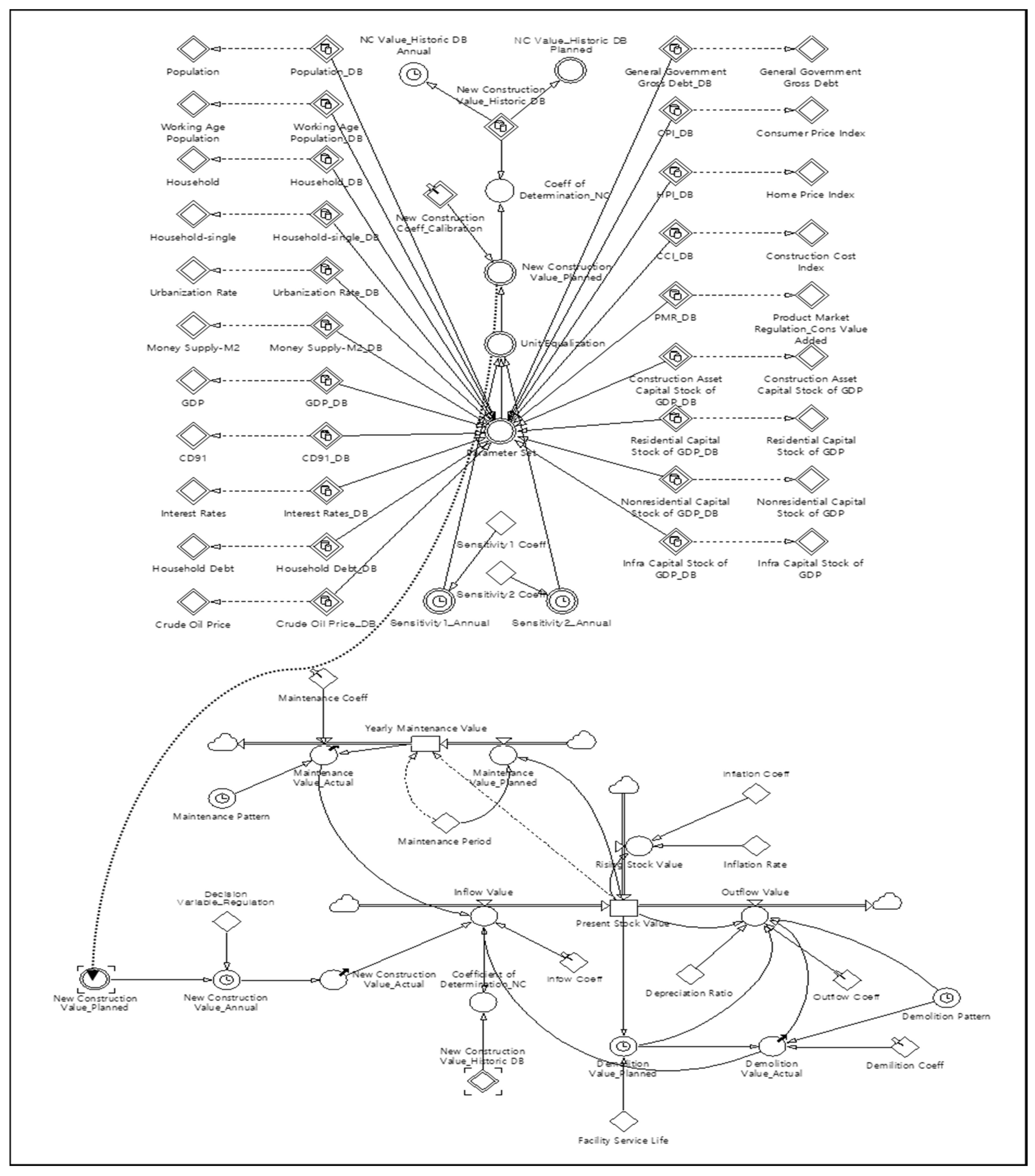
4.2.2. Structure of Simulation Module I

Module I is an analysis module for the possibility of new demand for construction in response to dynamic changes in socio-economic, institutional, and quantitative factors for the construction market. The input variables are social factors such as total population, the number of people who can produce, the total number of households, the number of households with 1 to 2 people, city of urbanization, currency amount, gross domestic product, international oil prices, and residential price to income ratio. Institutional economic factors include interest rate, family debt ratio, national debt ratio, consumer price index, construction cost index, residential price index, and market regulation index. Physical factors include the total ratio of construction capital stock to GDP, the total ratio of residential construction capital stock to GDP, the total ratio of construction capital stock to non-residential GDP, and the total ratio of construction capital stock to GDP (Figure 6).

4.2.3. Structure of Simulation Module II

The maintenance market can be divided into a routine maintenance market and a market where large-scale maintenance reinforcement occurs. The daily maintenance market is a small-scale market, which is frequent but small in cost. A market where large-scale reinforcement occurs can be called a multiple case market, with low frequency but high construction costs. The effective maintenance market in this study is targeted at areas where suppliers can enter a business that does not include the routine maintenance market. The time when large-scale repair and reinforcement occurs is set as 20 years having elapsed since the completion of the rapid decline in facility function (Figure 6).

The main level variable called construction capital stock is the new construction demand, maintenance demand, demolition demand, and the vertical axis change rate variable. The sub-level variable called annual maintenance amount is determined by the rate of change in the amount of maintenance compared to the current amount in the following year.

4.2.4. Formulae of Modules

The process of conceptualizing and formulating the model structure’s formulae and converting it into a stock-flow form that can be computer-simulated through formalization is presented below. The construction stock (present stock value, $P{V}_t$) at the time t is composed of the total amount of input $I{V}_{t-s}$ in the past year (t-s) that reflects the depreciation rate ($r_t$) in the input value ($\mathrm{I}{V}_t$) of the construction year. The estimate of the construction capital stock amount can be expressed as Equation (1).

$$P{V}_t=\mathrm{I}{V}_t+\left(1-r_t\right)I{V}_{t-1}+\left(1-r_t\right)\left(1-r_{t-1}\right)I{V}_{t-2}+\cdots +\left(1-r_t\right)\cdots \left(1-r_{t-s+1}\right)I{V}_{t-s}$$

(1)

$P{V}_t$: Construction capital stock amount

$\mathrm{I}{V}_t$: Construction capital input

$r_t$: depreciation rate

Assuming that the depreciation form follows the declining rate method since the depreciation rate is constant every year, Equation (1) can be expressed simply as Equation (2) below, and the left side is defined as the right side.

$$PS{V}_{t-1}=I{V}_{t-1}+\left(1-r_{t-1}\right)I{V}_{t-2}+{\left(1-r_{t-1}\right)}^{2}I{V}_{t-3}+\cdots {\left(1-r_{t-1}\right)}^{s}I{V}_{t-\left(s+1\right)}$$

(2)

The time for large-scale maintenance of residential buildings is set to 20 years after completion, and the service life of facilities is 49.84 years [44]. The construction stock amount consisting of the new amount, maintenance amount, and demolition amount of the residential sector is expressed as Equation (3).

$$RPS{V}_t=N{V}_t+{{\displaystyle \int }}_{t_0}^t[{\left(1-r_t\right)}^{t}PS{V}_{t-1}]dt+M{V}_t+D{V}_t$$

(3)

The amount of new construction is generated through optimal parameter estimation using inputs of changes in explanatory environmental variables such as various societies, economies, and institutions, and the parameters are searched to optimize the results of the simulation model. The formula for the amount of new residential construction is presented in Equation (4).

$$N{V}_t={\alpha }_1{x}_{1t}+{\alpha }_{2t}{x}_{2t}+\cdots +{\alpha }_{nt}{x}_{nt}+c_{it}={\displaystyle \sum }_{i=1}^n{\alpha }_{it}{x}_{it}+c_{it}$$

(4)

${\alpha }_i$: parameter(d), $x_i$: variable(d), $c_i$: constant(d)

It is difficult to say that the planned maintenance amount will be converted into the actual maintenance amount due to realistic constraints such as a limited budget [45]. The actual amount of maintenance construction is estimated through the additional correction process of the maintenance pattern coefficient and the conversion coefficient to apply the ratio of the cost of maintenance to the new construction cost.

The ratio of the cost of maintenance to new construction ranges from 95% to 100% for horizontal expansion, from 85% to 90% for vertical expansion, is about 80% for houses undergoing full-scale remodeling, and from 60% to 70% for the non-housing stock. The residential construction market corrects the cost conversion factor to 80% (Equation (5)).

$$M{V}_t=\frac{1}{1-\alpha e^{bt}}\times PS{V}_{t-10}, \alpha =0.16, b=0.1\left(49.84\ge t-to\ge 20\right)$$

(5)

As with the maintenance amount, it is difficult to say that the planned demolition amount will be converted to the actual demolition amount due to realistic restrictions. The actual amount of demolition construction is estimated through the additional correction process of the demolition pattern coefficient and the conversion coefficient to apply the ratio of the cost of demolition to the new construction cost. The ratio of the cost of demolition is generally within 3% of the cost of repair work, 3.48% in the Public Procurement Service (2017), and 3.2% in the Korea Institute of Construction Technology (2013). This study will correct the conversion ratio of 3.2% to the demolition scale (Equation (6)).

$$D{V}_t=\frac{1}{1+\alpha e^{bt}}\times PS{V}_{t-10}, \alpha =0.02, b=0.06\left(t-to\ge 49.84\right)$$

(6)

4.3. Model Validation

Objectivity verification is a process that examines how well the model represents the problem. It is the process of assigning objectivity and securing reliability.

The objectivity of the model is verified by comparing the model with actual data. In this study, the regression model’s least square method was used to verify the model’s objectivity. Also, the simulation result of the model was verified by using the coefficient of determination ($R^2$). The coefficient of determination ($R^2$) means the ratio of the variance of the actual data explained by the results simulated through the model. The coefficient of determination ranges between 0 and 1. If a model has a value close to 0, it is low in usefulness. However, the larger the value of the coefficient of determination, the higher the usefulness of the model.

As a result of analyzing the $R^2$ based on the simulation result, the $R^2$ for the new amount in the residential construction market is 0.82 (

Table 7. Objectivity verification results of estimating the size of new construction market.

Division			N	Average	Standard Deviation	${\mathit{R}}^2$
Residential	New construction amount	Actual data	16	52.42	5.84	0.82
		Simulation	16	52.39	4.63

).

5. Simulation Output of Demand Forecasting

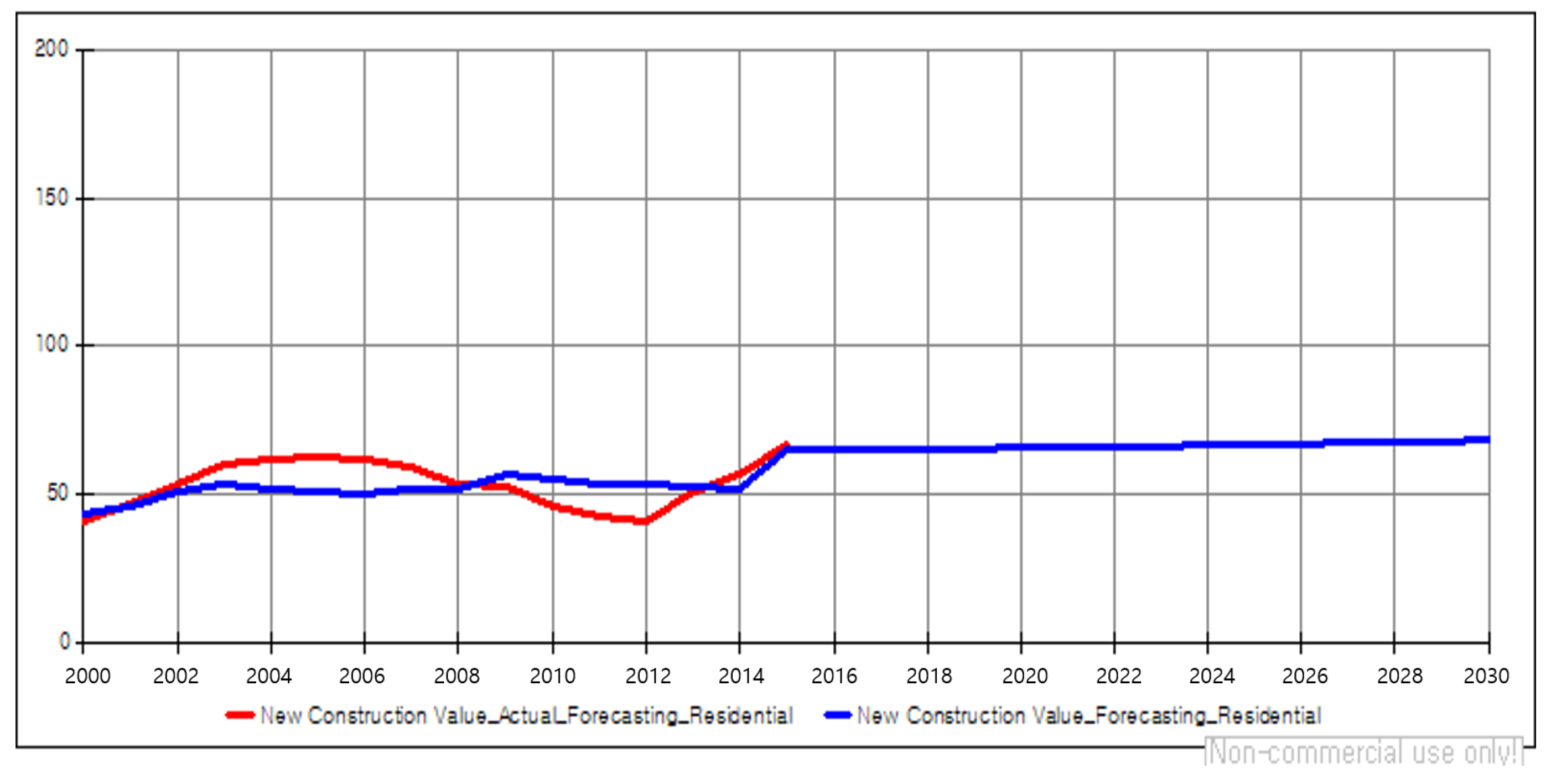
5.1. Results of the Construction Demand Forecasting Model

According to forecasting, the residential construction market, based on simulation, is expected to increase by about 1 trillion won in 5-year increments from 70 trillion won in 2015. According to the market forecast results in new construction, maintenance, and demolition stages, demand is expected to increase mainly in the maintenance market. In the domestic construction market, as the demand for maintenance surges, the proportion of maintenance work is projected to be 40%, similar to that of developed countries (Lee, 2017). It is projected that the restructuring of old buildings and old infrastructure, including residential, will gradually increase the new construction market (Lee, 2017). The research model has a high level of explanatory power to reality in that the expansion trend of the demolition market for reinvestment projects such as reconstruction and redevelopment has been partially confirmed through the model’s demand forecast results. The long-term domestic construction market’s demand forecast results are in

Table 8. Forecasting results of the scale forecasting model in construction market.

Engineering Type	Stage	2015	2016	2017	2018
Residential	New	65 trillion won	67 trillion won	68 trillion won	69 trillion won
	Maintenance	4.0 trillion won	4.8 trillion won	6.0 trillion won	8.8 trillion won
	Demolition	0.99 trillion won	0.10 trillion won	0.12 trillion won	0.14 trillion won
	Total	69.3 trillion won	71.7 trillion won	74.2 trillion won	78.5 trillion won

and Figure 7.

5.2. Sensitivity Analysis of Construction Demand Forecasting Model

The sensitivity of the model is analyzed based on the influence of variables. For the residential construction market, the sensitivity was low due to the sensitivity analysis of the changes in the ratio of construction stock to GDP and the useful life of each facility. It can be interpreted that the above variables have low sensitivity because there is no uncertainty in the structure constituting the system. The sensitivity of multivariate, which performed a sensitivity analysis of the interest rate and four variables simultaneously, is relatively high. From the above results it can be inferred that the new construction market’s demand may expand or contract as the household loan rate increases. Even if the variable’s sensitivity fluctuation range is expanded from ±20% to ±30%, the simulation result and change pattern show a specific pattern. Thus, the relationship between the set variables and the suitability of the model appears to be secured (

Table 9. Variables of sensitivity analysis.

Variables		Random Model	Min	Max
Residential	Interest rate	Random uniform	−20%	+20%
	Construction capital stock	Random uniform	−20%	+20%
	Facility service life	Random uniform	−10%	+10%
	Market regulation	Random uniform	−20%	+20%

). Also, it is essential to control the interest rate variable in the residential construction market because the market’s effect is mainly due to changes in that variable (Figure 8).

6. Conclusions

The construction market is a vast system composed of many subsystems, dynamic due to the interaction between them. The system has complex system characteristics due to various environmental factors surrounding the construction market and dynamic construction paradigm changes. Forecasting the demand for the future construction market is significant because it has a profound effect on overall construction activities. It is not easy to make scientific predictions considering dynamic market trends and environmental changes because various factors affecting the construction market occur in a complicated way.

This study aimed to identify how the construction market will change in the long term by developing a model for predicting construction demand. Also, to achieve the model’s usefulness and usability, the factors for the phenomenon are analyzed through simulation.

This study analyzes the mutual impact relationship of demand influencing and influencing factors, mainly in the domestic residential construction market. Through a systematic approach, the construction market’s structure is analyzed, and the usefulness of the model is verified. Also, by using the research model to forecast future changes in construction market demand, we confirm how much quantitative growth is possible in the market.

According to the forecasted results of this study’s model, the domestic residential construction market is expected to grow in the future based on the maintenance market’s rapid growth. Using the model, we provide the prediction results of the scale of the future construction market according to changes in social, economic, and institutional environmental factors. The results of this study support strategy establishment and rational decision-making according to various environmental factors such as changes in the form of demand or the emergence of new markets.

The model cannot accurately analyze and interpret the market structure from the beginning. Based on the initial model, the model should be developed through continuous system structure improvement. Through further developments, it is expected that the reliability of the model can be improved by analyzing variables that affect the entire construction market as well as variables that affect each specialized market.

References

- Kwon, O.H.; Choi, M.S. Mid-to Long-Term Market Outlook by Construction Product (II)-Non-Residential Sector; Construction & Economy Research Institute of Korea: Seoul, Korea, 2004. [Google Scholar]
- Jin, K.H.; Lee, K.S.; Lee, S.K.; Yang, J.S.; Kim, H.W.; Kim, S.G. Construction Industry Policy Service Platform (II)—Analysis and Forecast of Construction Business; Korea Institute of Civil Engineering and Building Technology: Seoul, Korea, 2015. [Google Scholar]
- Jin, K.H.; Park, H.G.; Lee, S.K.; Kim, S.J. Development of Construction Market Analysis and Forecasting Model (III); Korea Institute of Civil Engineering and Building Technology: Seoul, Korea, 2013. [Google Scholar]
- Park, S.H.; Youn, S.J.; Kim, S.W. The Application of SD for Supply & Demand Plan of Manpower -in case of Information Security industry for the UIT Environment. Korea Syst. Dyn. Soc. 2003, 4, 93–119. [Google Scholar]
- Kim, D.G.; Won, J.Y. Development of Foresight Method for Future Disaster through the Analysis of Complex Foresight Methodology; National Disaster Management Institute: Seoul, Korea, 2013. [Google Scholar]
- Public Procurement Service. Analysis of Construction Cost by Public Building Type in 2016; Public Procurement Service: Seoul, Korea, 2017.
- Park, K.Y. Development of Financial Feasibility Analysis Model Using Stochastic System Dynamics Method in a Hotel Development Project. Ph.D. Thesis, University of Hanyang, Seoul, Korea, 2012. [Google Scholar]
- Kim, J.Y.; Kim, M.C. A Study on the Development of the Forecasting Model for the Construction Industry Considering the Economic Structure Change; Korea Research Institute for Human Settlements: Seoul, Korea, 2000. [Google Scholar]
- Kim, J.Y.; Kim, S.I.; Lee, H.C. Structural Change and Prospects in the Construction Industry; Korea Research Institute for Human Settlements: Seoul, Korea, 2001. [Google Scholar]
- Kim, J.H. An Analytical Model for Labor Supply and Demand in Construction. Ph.D. Thesis, University of Ajou, Suwon, Korea, 2008. [Google Scholar]
- Kim, K.H.; Lee, H.S.; Kwon, J.A.; Choi, S.H. A Study on the Residential Forecasting Model V.; Korea Residential Institute: Seoul, Korea, 2008. [Google Scholar]
- Moon, T.H. Sustainable City as a System Accident; Jipmoon: Seoul, Korea, 2002. [Google Scholar]
- Moon, T.H. Issues and Methodological Status of System Dynamics; Korea System Dynamics Society: Seoul, Korea, 2007. [Google Scholar]
- Kim, Y.W. Analysis of Construction Management Market Using System Thinking; Korea Society of Civil Engineering: Seoul, Korea, 2010. [Google Scholar]
- Park, M.S.; An, C.B.; Lee, H.S.; Hwang, S.J. Analysis of the Korean Residential Market Mechanisms and Residential Sales Policies Using System Dynamics. Korea Inst. Constr. Eng. Manag. 2009, 10, 42–52. [Google Scholar]
- Shin, D.H. The Prediction of Long-Term Residential Market and Improvement of Its Policy. Ph.D. Thesis, University of Kangwon, Gangwondaehak-gil, Korea, 2013. [Google Scholar]
- Korea Institute of Science and Technology Evaluation and Planning. Ripple Effect Analysis of Government R&D Investment by System Approach; Korea Institute of Science and Technology Evaluation and Planning: Seoul, Korea, 2015. [Google Scholar]
- Park, M.S. Model-based Dynamic Resource Management for Construction Projects. Autom. Constr. 2005, 14, 585–598. [Google Scholar] [CrossRef]
- Onat, N.C.; Egilmez, G.; Tatari, O. Towards Greening the US Residential Building Stock: A System Dynamics Approach. Build. Environ. 2014, 78, 68–80. [Google Scholar] [CrossRef]