
A Deep Neural Network Model for Speaker Identification


Abstract
1. Introduction
Related Work
2. Materials and Methods
2.1. Background
2.1.1. Recurrent Neural Network
2.1.2. Long Short-Term Memory (LSTM)
2.1.3. Gated Recurrent Unit (GRU)
2.1.4. Convolutional Neural Network (CNN)
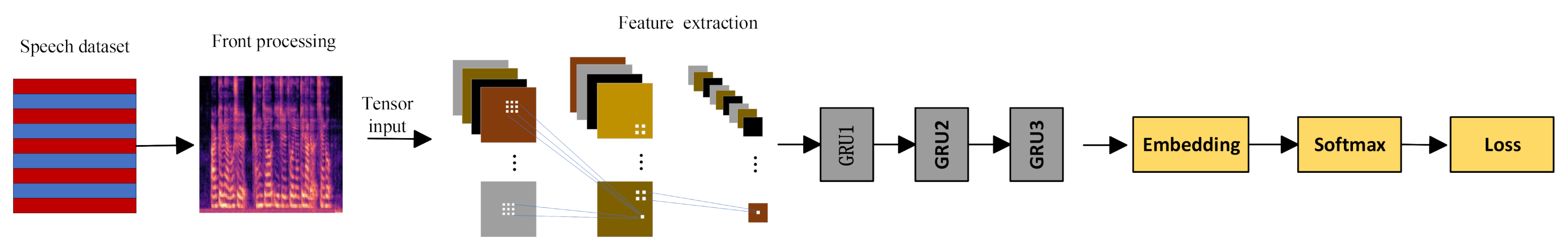
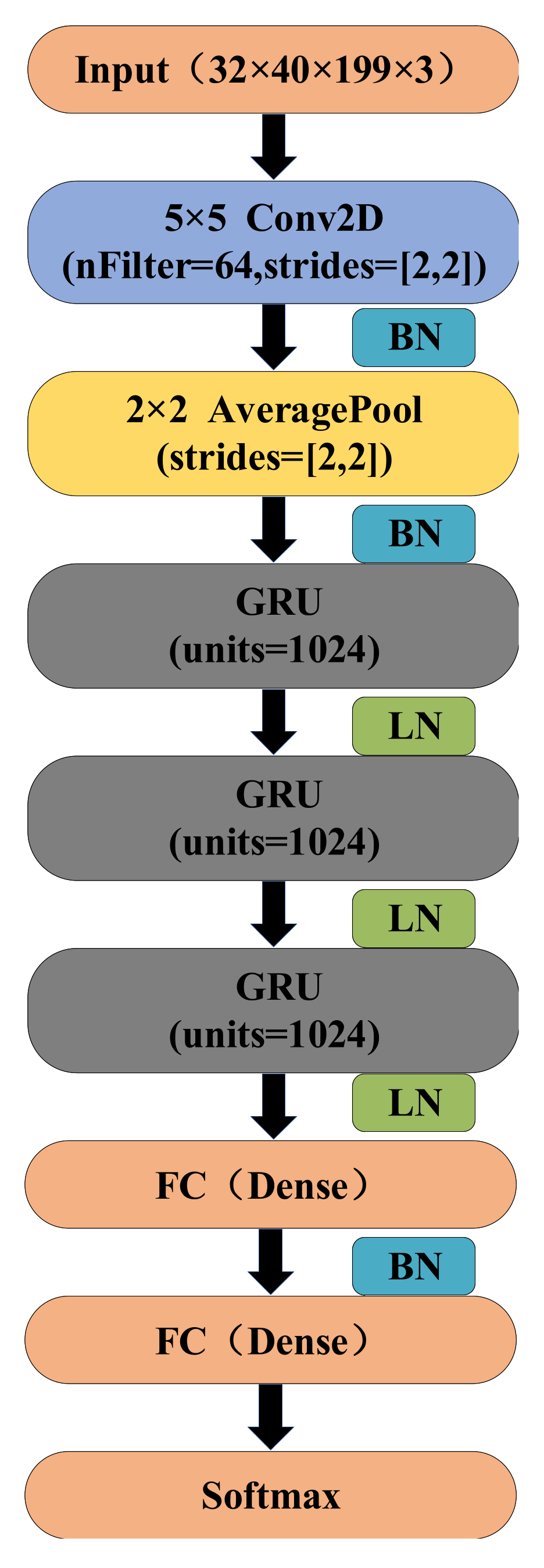
2.2. Model Overview
Deep GRU Architecture
2.3. Experimental Setup
2.3.1. Speech Dataset
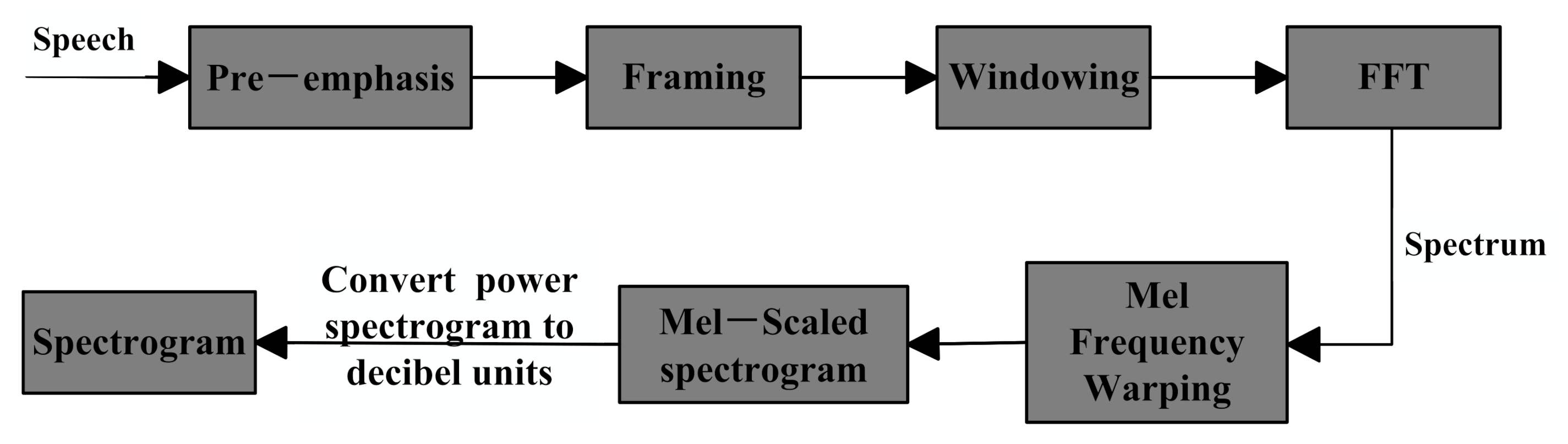
2.3.2. Data Preprocessing
3. Results
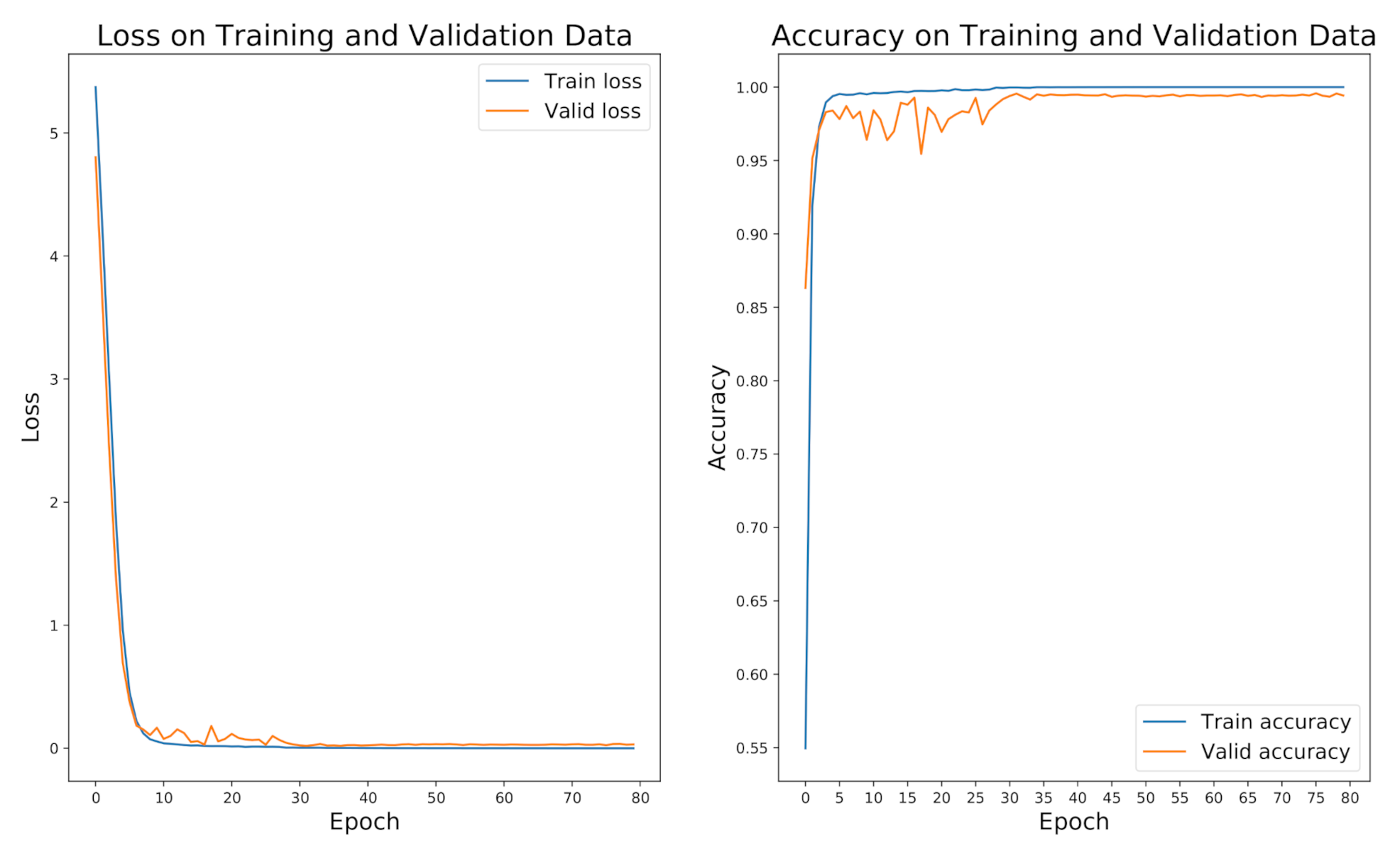
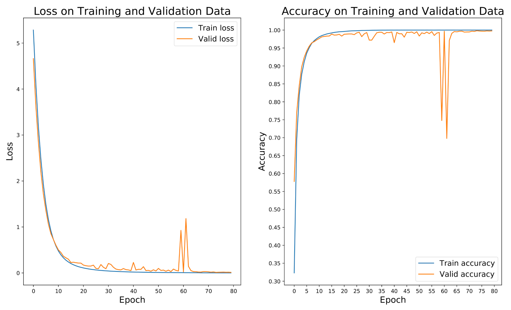
3.1. Training
3.2. Evaluation Metrics
3.3. Model Results
4. Conclusions
Author Contributions
Funding
Institutional Review Board Statement
Informed Consent Statement
Data Availability Statement
Conflicts of Interest
References
- Tomi, K.; Li, H. An Overview of Text-Independent Speaker Recognition: From Features to Supervectors. Speech Commun. 2010, 52, 12–40. [Google Scholar]
- Sadaoki, F. Recent Advances in Speaker Recognition. Pattern Recognit. Lett. 1997, 18, 859–872. [Google Scholar]
- Reynolds, D.A. An Overview of Automatic Speaker Recognition Technology. In Proceedings of the 2002 IEEE International Conference Acoust. Speech Signal Process, Orlando, FL, USA, 13–17 May 2002; Volume 4, pp. 4072–4075. [Google Scholar]
- Campbell, J.P., Jr. Speaker Recognition: A Tutorial. Proc. IEEE 1997, 85, 1437–1462. [Google Scholar] [CrossRef]
- Reynolds, D.A.; Rose, R.C. Robust text-independent speaker identification using Gaussian mixture speaker models. IEEE Trans. Speech Audio Process. 1995, 3, 72–83. [Google Scholar] [CrossRef]
- Togneri, R.; Pullella, D. An Overview of Speaker Identification: Accuracy and Robustness Issues. IEEE Circuits Syst. Mag. 2011, 11, 23–61. [Google Scholar] [CrossRef]
- Li, B. On identity authentication technology of distance education system based on voiceprint recognition. In Proceedings of the 30th Chinese Control Conference, Yantai, China, 22–24 July 2011; pp. 5718–5721. [Google Scholar]
- Chen, Y.-H.; Ignacio, L.-M.; Sainath, T.N.; Mirkó, V.; Raziel, A.; Carolina, P. Locally-connected and convolutional neural networks for small footprint speaker; recognition. In Proceedings of the Sixteenth Annual Conference of the International Speech Communication Association, Dresden, Germany, 6–10 September 2015. [Google Scholar]
- Parveen, S.; Qadeer, A.; Green, P. Speaker recognition with recurrent neural networks. In Proceedings of the Sixth International Conference on Spoken Language Processing, Beijing, China, 16–20 October 2000. [Google Scholar]
- Ankur, M.; Divya, K.; Agarwal, R.K. Speaker recognition for Hindi speech signal using MFCC-GMM approach. Procedia Comput. Sci. 2018, 125, 880–887. [Google Scholar]
- Ren, J.; Hu, Y.; Tai, Y.-W.; Wang, C.; Xu, L.; Sun, W.; Yan, Q. Look, listen and learn—A multimodal LSTM for speaker identification. In Proceedings of the AAAI Conference on Artificial Intelligence, Phoenix, AZ, USA, 12–17 February 2016; Volume 30. [Google Scholar]
- Bu, H.; Du, J.; Na, X.; Wu, B.; Zheng, H. AISHELL-1: An open-source Mandarin speech corpus and a speech recognition baseline. In Proceedings of the 2017 20th Conference of the Oriental Chapter of the International Coordinating Committee on Speech Databases and Speech I/O Systems and Assessment (O-COCOSDA), Seoul, Korea, 1–3 November 2017; pp. 1–5. [Google Scholar]
- Minsky, M. Steps toward Artificial Intelligence. Proc. IRE 1961, 46, 8–30. [Google Scholar] [CrossRef]
- Jordan, M.I.; Mitchell, T.M. Machine learning: Trends, perspectives, and prospects. Science 2015, 349, 255–260. [Google Scholar] [CrossRef]
- Wang, L.; Minami, K.; Yamamoto, K.; Nakagawa, S. Speaker Identification by Combining MFCC and Phase Information in Noisy Environments. In Proceedings of the 2010 IEEE International Conference on Acoustics, Speech and Signal Processing, Dallas, TX, USA, 14–19 March 2010; pp. 4502–4505. [Google Scholar] [CrossRef]
- Gudnason, J.; Brookes, M. Voice source cepstrum coefficients for speaker identification. In Proceedings of the 2008 IEEE International Conference on Acoustics, Speech and Signal Processing, Las Vegas, NV, USA, 31 March–4 April 2008; pp. 4821–4824. [Google Scholar] [CrossRef]
- Lawson, A.; Vabishchevich, P.; Huggins, M.; Ardis, P.; Battles, B.; Stauffer, A. Survey and Evaluation of Acoustic Features for Speaker Recognition. In Proceedings of the 2011 IEEE International Conference on Acoustics, Speech and Signal Processing (ICASSP), Prague, Czech Republic, 22–27 May 2008; pp. 5444–5447. [Google Scholar] [CrossRef]
- Georgescu, A.; Cucu, H. GMM-UBM Modeling for Speaker Recognition on a Romanian Large Speech Corpora. In Proceedings of the 2018 International Conference on Communications (COMM), Bucharest, Romania, 14–16 June 2018; pp. 547–551. [Google Scholar] [CrossRef]
- Shahin, I. Speaker Identification in the Shouted Environment Using Suprasegmental Hidden Markov Models. Signal Process. 2008, 88, 2700–2708. [Google Scholar] [CrossRef][Green Version]
- Khan, M.A.; Kim, Y. Deep Learning-Based Hybrid Intelligent Intrusion Detection System. Comput. Mater. Contin. 2021, 68, 671–687. [Google Scholar] [CrossRef]
- Shafik, A.; Sedik, A.; Abd El-Rahiem, B.; El-Rabaie, E.-S.M.; El Banby, G.M.; Abd El-Samie, F.E.; Khalaf, A.A.M.; Song, O.-Y.; Iliyasu, A.M. Speaker identification based on Radon transform and CNNs in the presence of different types of interference for Robotic Applications. Appl. Acoust. 2021, 177, 107665. [Google Scholar] [CrossRef]
- Lukic, Y.; Vogt, C.; Dürr, O.; Stadelmann, T. Speaker Identification and Clustering Using Convolutional Neural Networks. In Proceedings of the 2016 IEEE 26th International Workshop on Machine Learning for Signal Processing (MLSP), Vietri sul Mare, Italy, 13–16 September 2016; pp. 1–6. [Google Scholar] [CrossRef]
- Hochreiter, S.; Schmidhuber, J. Long Short-Term Memory. Neural Comput. 1997, 9, 1735–1780. [Google Scholar] [CrossRef]
- Graves, A.; Jaitly, N.; Mohamed, A. Hybrid speech recognition with Deep Bidirectional LSTM. In Proceedings of the 2013 IEEE Workshop on Automatic Speech Recognition and Understanding, Olomouc, Czech Republic, 8–12 December 2013; pp. 273–278. [Google Scholar] [CrossRef]
- Mikolov, T.; Karafiát, M.; Burget, L.; Cernocký, J.; Khudanpur, S. Recurrent Neural Network Based Language Model. In Proceedings of the INTERSPEECH 2010 11th Annual Conference of the International Speech Communication Association, Makuhari, Chiba, Japan, 26–30 September 2010; pp. 1045–1048. [Google Scholar]
- Gelly, G.; Gauvain, J.-L.; Le, V.B.; Messaoudi, A. A Divide-and-Conquer Approach for Language Identification Based on Recurrent Neural Networks. In Proceedings of the INTERSPEECH, San Francisco, CA, USA, 8–12 September 2016; pp. 3231–3235. [Google Scholar]
- Gers, F.A.; Schmidhuber, E. LSTM recurrent networks learn simple context-free and context-sensitive languages. IEEE Trans. Neural Netw. 2001, 12, 1333–1340. [Google Scholar] [CrossRef]
- Graves, A.; Liwicki, M.; Fernández, S.; Bertolami, R.; Bunke, H.; Schmidhuber, J. A Novel Connectionist System for Unconstrained Handwriting Recognition. IEEE Trans. Pattern Anal. Mach. Intell. 2009, 31, 855–868. [Google Scholar] [CrossRef]
- Eyben, F.; Wöllmer, M.; Schuller, B.; Graves, A.; Schlüter, R.; Ney, H. From speech to letters—Using a novel neural network architecture for grapheme based ASR. In Proceedings of the 2009 IEEE Workshop on Automatic Speech Recognition & Understanding, Moreno, Italy, 13 November–17 December 2009; pp. 376–380. [Google Scholar] [CrossRef]
- Wollmer, M.; Eyben, F.; Schuller, B.; Rigoll, G.; Ney, H. A Multi-Stream ASR Framework for BLSTM Modeling of Conversational Speech. In Proceedings of the 2011 IEEE International Conference on Acoustics, Speech and Signal Processing (ICASSP), Prague, Czech Republic, 22–27 May 2011; pp. 4860–4863. [Google Scholar] [CrossRef]
- Kim, S.; Kim, I.; Vecchietti, L.F.; Har, D. Pose Estimation Utilizing a Gated Recurrent Unit Network for Visual Localization. Appl. Sci. 2020, 10, 8876. [Google Scholar] [CrossRef]
- Zhang, X.; Kuehnelt, H.; De Roeck, W. Traffic Noise Prediction Applying Multivariate Bi-Directional Recurrent Neural Network. Appl. Sci. 2021, 11, 2714. [Google Scholar] [CrossRef]
- Althelaya, K.A.; El-Alfy, E.M.; Mohammed, S. Stock market forecast using multivariate analysis with bidirectional and stacked (LSTM, GRU). Proceeding of the 2018 21st Saudi Computer Society National Computer Conference (NCC), Riyadh, Saudi Arabia, 25–26 April 2018; pp. 1–7. [Google Scholar]
- Liu, D.-R.; Lee, S.-J.; Huang, Y.; Chiu, C.-J. Air pollution forecasting based on attention-based LSTM neural network and ensemble learning. Expert Syst. 2020, 37, e12511. [Google Scholar] [CrossRef]
- Nagrani, A.; Chung, J.S.; Zisserman, A. Voxceleb: A large-scale speaker identification dataset. arXiv 2017, arXiv:1706.08612. [Google Scholar]
- Zhang, Y.; Pezeshki, M.; Brakel, P.; Zhang, S.; Bengio, C.L.Y.; Courville, A. Towards end-to-end speech recognition with deep convolutional neural networks. arXiv 2017, arXiv:1701.02720. [Google Scholar]
- Wang, Y.; Deng, X.; Pu, S.; Huang, Z. Residual convolutional CTC networks for automatic speech recognition. arXiv 2017, arXiv:1702.07793. [Google Scholar]
- Amodei, D.; Ananthanarayanan, S.; Anubhai, R.; Bai, J.; Battenberg, E.; Case, C.; Casper, J.; Catanzaro, B.; Cheng, Q.; Chen, G.; et al. Deep speech 2: End-to-end speech recognition in english and mandarin. In Proceedings of the International Conference on Machine Learning, PMLR, New York, NY, USA, 20–22 June 2016; pp. 173–182. [Google Scholar]
- Sainath, T.N.; Weiss, R.J.; Senior, A.; Wilson, K.W.; Vinyals, O. Learning the speech front-end with raw waveform CLDNNs. In Proceedings of the Sixteenth Annual Conference of the International Speech Communication Association, Dresden, Germany, 6–10 September 2015. [Google Scholar]
- Sak, H.; Senior, A.W.; Beaufays, F. Long Short-Term Memory Based Recurrent Neural Network Architectures for Large Vocabulary Speech Recognition. arXiv 2014, arXiv:1402.1128. [Google Scholar]
- Liu, Y.; Hou, D.; Bao, J.; Qi, Y. Multi-step Ahead Time Series Forecasting for Different Data Patterns Based on LSTM Recurrent Neural Network. In Proceedings of the 2017 14th Web Information Systems and Applications Conference (WISA), Liuzhou, China, 11–12 November 2017; pp. 305–310. [Google Scholar]
- Cho, K.; van Merrienboer, B.; Gulcehre, C.; Bahdanau, D.; Bougares, F.; Schwenk, H.; Bengio, Y. Learning Phrase Representations Using RNN Encoder–Decoder for Statistical Machine Translation. arXiv 2014, arXiv:1406.1078. [Google Scholar]
- Manabe, K.; Asami, Y.; Yamada, T.; Sugimori, H. Improvement in the Convolutional Neural Network for Computed Tomography Images. Appl. Sci. 2021, 11, 1505. [Google Scholar] [CrossRef]
- Lin, Y.-Y.; Zheng, W.-Z.; Chu, W.C.; Han, J.-Y.; Hung, Y.-H.; Ho, G.-M.; Chang, C.-Y.; Lai, Y.-H. A Speech Command Control-Based Recognition System for Dysarthric Patients Based on Deep Learning Technology. Appl. Sci. 2021, 11, 2477. [Google Scholar] [CrossRef]
- Lu, W.; Zhang, Q. Deconvolutive Short-Time Fourier Transform Spectrogram. IEEE Signal Process. Lett. 2009, 16, 576–579. [Google Scholar] [CrossRef]
- Naderi, N.; Nasersharif, B. Ultiresolution convolutional neural network for robust speech recognition. In Proceedings of the 2017 Iranian Conference on Electrical Engineering (ICEE), Tehran, Iran, 2–4 May 2017; pp. 1459–1464. [Google Scholar] [CrossRef]
- Fei, Z.; Zhang, J.-S. Softmax Discriminant Classifier. In Proceedings of the 2011 Third International Conference on Multimedia Information Networking and Security, Shanghai, China, 4–6 November 2011; pp. 16–19. [Google Scholar]
- Ioffe, S.; Szegedy, C. Batch Normalization: Accelerating Deep Network Training by Reducing Internal Covariate Shift. In Proceedings of the 32nd International Conference on Machine Learning, Lille, France, 7–9 July 2015; pp. 448–456. [Google Scholar]
- Ba, J.L.; Kiros, J.R.; Hinton, G.E. Layer normalization. arXiv 2016, arXiv:1607.06450. [Google Scholar]
- Glorot, X.; Bordes, A.; Bengio, Y. Deep Sparse Rectifier Neural Networks. In Proceedings of the Fourteenth International Conference on Artificial Intelligence and Statistics, Fort Lauderdale, FL, USA, 11–13 April 2011; Volume 15, pp. 315–323. [Google Scholar]
- Maas, A.L.; Hannun, A.Y.; Ng, A.Y. Rectifier nonlinearities improve neural network acoustic models. Proc. Icml 2013, 30, 3. [Google Scholar]
- Hestness, J.; Narang, S.; Ardalani, N.; Diamos, G.; Jun, H.; Kianinejad, H.; Patwary, M.; Ali, M.; Yang, Y.; Zhou, Y. Deep learning scaling is predictable, empirically. arXiv 2017, arXiv:1712.00409. [Google Scholar]
- Gowdy, J.N.; Tufekci, Z. Mel-scaled discrete wavelet coefficients for speech recognition. In Proceedings of the 2000 IEEE International Conference on Acoustics, Speech and Signal Processing, Proceedings (Cat. No.00CH37100). Istanbul, Turkey, 5–9 June 2000; Volume 3, pp. 1351–1354. [Google Scholar] [CrossRef]
- Van Der Walt, S.; Colbert, S.C.; Varoquaux, G. The NumPy Array: A Structure for Efficient Numerical Computation. Comput. Sci. Eng. 2011, 13, 22–30. [Google Scholar] [CrossRef]
- Ruder, S. An overview of gradient descent optimization algorithms. arXiv 2016, arXiv:1609.04747. [Google Scholar]
- Dozat, T. Incorporating Nesterov Momentum into Adam. 2016. Available online: https://openreview.net/forum?id=OM0jvwB8jIp57ZJjtNEZ (accessed on 19 January 2016).
- Feng, Y.; Cai, X.; Ji, R. Evaluation of the deep nonlinear metric learning based speaker identification on the large scale of voiceprint corpus. In Proceedings of the 2016 10th International Symposium on Chinese Spoken Language Processing (ISCSLP), Tianjin, China, 17–20 October 2016; pp. 1–4. [Google Scholar]


| Speakers | Utterances | Ratio | |
|---|---|---|---|
| Training data | 400 | 127,551 | 90% |
| Validation data | 400 | 7278 | 5% |
| Test data | 400 | 7096 | 5% |
| Types of Model | Datasets | Overall Accuracy (%) | Real Time per Epoch |
|---|---|---|---|
| 2-D CNN | Aishell-1 | 95.42% | 1035 s |
| noise-added Aishell-1 | 48.57% | ||
| CNN + original RNN | Aishell-1 | 96.67% | 1154 s |
| noise-added Aishell-1 | 55.29% | ||
| CNN + RNN-LSTM cell | Aishell-1 | 97.09% | 1065 s |
| noise-added Aishell-1 | 70.42% | ||
| Proposed Deep GRU | Aishell-1 | 98.96% | 980 s |
| noise-added Aishell-1 | 91.56% |
| Methods | Datasets | Overall Accuracy (%) |
|---|---|---|
| Proposed Deep GRU | Aishell-1 | 98.96% |
| Aishell-1 with Gaussian white noise added | 91.56% | |
| MFCC-GMM [10] | Aishell-1 | 86.29% |
| Aishell-1 with Gaussian white noise added | 55.29% | |
| CNN [8] | Aishell-1 | 92.45% |
| Aishell-1 with Gaussian white noise added | 62.39% | |
| RNN [9] | Aishell-1 | 89.67% |
| Aishell-1 with Gaussian white noise added | 58.29% | |
| Multimodal LSTM [11] | Aishell-1 | 96.25% |
| Aishell-1 with Gaussian white noise added | 70.42% |
| Layer Name | Struct | Stride | Param# |
|---|---|---|---|
| Input | 32 × 40 × 199 × 3 | - | - |
| 2-D Conv | 5 × 5 kernel, 64 filter | 2 × 2 | 4.8 k |
| Average pooling | 2 × 2 pooling | 2 × 2 | 0 |
| RNN | 1024 cell | - | 2.4 m |
| RNN | 1024 cell | - | 2.1 m |
| RNN | 1024 cell | - | 2.1 m |
| average | - | - | 0 |
| Dense | 1024 × 512 | - | 0.52 m |
| Length Normalization | - | - | 0.2 m |
| Output (softmax) | 1024 × 400 | - | 0 |
| Total | - | - | 7.32 m |
| Layer Name | Struct | Stride | Param# |
|---|---|---|---|
| Input | 32 × 40 × 199 × 3 | - | - |
| 2-D Conv | 5 × 5 kernel, 64 filter | 2 × 2 | 4.8 k |
| Average pooling | 2 × 2 pooling | 2 × 2 | 0 |
| LSTM | 1024 units | - | 9.4 m |
| LSTM | 1024 units | - | 8.3 m |
| LSTM | 1024 units | - | 8.3 m |
| average | - | - | 0 |
| Dense | 1024 × 512 | - | 0.52 m |
| Length normalization | - | - | 0.2 m |
| Output (softmax) | 1024 × 400 | - | 0 |
| Total | - | - | 26.93 m |
| Layer Name | Struct | Stride | Param# |
|---|---|---|---|
| Input | 32 × 40 × 199 × 3 | - | - |
| 2-D Conv | 5 × 5 kernel, 64 filter | 2 × 2 | 4.8 k |
| Average pooling | 2 × 2 pooling | 2 × 2 | 0 |
| GRU | 1024 units | - | 5.1 m |
| GRU | 1024 units | - | 6.3 m |
| GRU | 1024 units | - | 6.3 m |
| average | - | - | 0 |
| Dense | 1024 × 512 | - | 0.52 m |
| Length normalization | - | - | 0.2 m |
| Output (softmax) | 1024 × 400 | - | 0 |
| Total | - | - | 18.42 m |
Publisher’s Note: MDPI stays neutral with regard to jurisdictional claims in published maps and institutional affiliations. |
© 2021 by the authors. Licensee MDPI, Basel, Switzerland. This article is an open access article distributed under the terms and conditions of the Creative Commons Attribution (CC BY) license (https://creativecommons.org/licenses/by/4.0/).
Share and Cite
Ye, F.; Yang, J. A Deep Neural Network Model for Speaker Identification. Appl. Sci. 2021, 11, 3603. https://doi.org/10.3390/app11083603
Ye F, Yang J. A Deep Neural Network Model for Speaker Identification. Applied Sciences. 2021; 11(8):3603. https://doi.org/10.3390/app11083603
Chicago/Turabian StyleYe, Feng, and Jun Yang. 2021. "A Deep Neural Network Model for Speaker Identification" Applied Sciences 11, no. 8: 3603. https://doi.org/10.3390/app11083603
APA StyleYe, F., & Yang, J. (2021). A Deep Neural Network Model for Speaker Identification. Applied Sciences, 11(8), 3603. https://doi.org/10.3390/app11083603