1. Introduction
The importance of power quality (PQ) in distribution networks continuously increases. One of the reasons is the integration of new device technologies on a large scale, like photovoltaic inverters, the transition from incandescent to LED lamps, and the integration of battery electric vehicles and smart distribution systems. This may result in an increased deterioration of PQ, which could in return affect other electronic devices, in particular if their sensitivity to a particular PQ phenomenon (e.g., harmonic distortion) is high (low immunity).
Increased levels of harmonic distortion can, for example, cause audible noise and additional losses in network elements and devices, resulting in additional thermal stress, which can result in reduced lifetime. Harmonic can also result in interference in communication, increased neutral conductor loading in LV networks, and reversible or irreversible malfunction of devices [
1,
2,
3].
The prices of PQ monitoring equipment have continuously decreased during the last decades. Especially the integration of intelligent electronic devices (IED), like energy meters, enables extremely cost-efficient solutions [
4]. Due to this trend, network operators have intensified their PQ measurement activities and the number of monitored sites rapidly increases. Consequently, the amount of PQ measurement data increases and its efficient management and analysis becomes a challenge of high complexity [
5]. As also identified by the CIRED/CIGRE working group C4.112 “Guidelines for Power quality monitoring” [
6], efficient methods and algorithms to analyze these large amounts of data are a key issue for future smart grids. Efficient and automated methods for processing large amounts of data are essential, but rarely exist at present.
Harmonic emission in public LV networks is mainly determined by the type and number of connected equipment with power electronic interfaces and depends on the behavior of the connected consumers/users (e.g., office hours) and the amount of generation (e.g., time of the day). Subsequently, PQ levels in public LV networks will vary over time and allow for the definition of distinctive emission profiles for harmonic currents. The different characteristics of these harmonic emission profiles can be used for the construction of a classification system for the identification of the probable consumer configuration based on the measurements of their harmonic currents.
Section 2 introduces the impact factors for PQ in public LV networks, as well as the typical variations within their time series. The German measurement campaign, which is the basis for the measurement data, is presented in the following section, highlighting the consumer configurations of the 40 measurement sites and the analyzed harmonic currents. The automatic generation of characteristic classes of typical harmonic emission profiles using measurements is explained in
Section 4. The design of a classification system using a binary decision tree in combination with support vector machines is part of
Section 5. The performance of the training and the testing process of the classification system is evaluated in
Section 6. The last section introduces a measure of misclassification, which allows the user of the classification system to identify emission profiles that are incorrectly assigned to the defined classes of emission profiles.
2. Impact Factors on Power Quality
The variety of factors influencing power quality can be generally allocated into the electrical and the non-electrical environment. The electrical environment includes all factors directly related to type and number of devices connected to the network and the network elements themselves [
7]. The non-electric environment includes all factors that have an additional impact, in particular on the usage behavior (e.g., climatic conditions) and the penetration ratio of electric devices.
2.1. Electrical Environment
Three different aspects represent the electrical environment at the measurement site. The consumer topology is characterized by the amount and type of consumers connected to the network, which is directly linked to the type and number of disturbing devices. The generation topology characterizes number, type, and rated power of the generating installations connected to the network. Most of the installations utilize inverters which can emit, for example, harmonics. Typical examples are photovoltaic installations. The network topology covers all characteristics directly related to the network. The technical parameters mainly influence the short circuit power, which determines the voltage quality levels for a given current emission.
2.2. Types of Variation
The impact of the electrical environment results in variations of different periods, which are displayed in
Figure 1 [
8].
Short-term variations are mainly influenced by the consumer usage and generation behavior of the connected devices. Certain consumer topologies show a distinct behavior with different daily patterns of current quality parameters (e.g., working days vs. weekends in office buildings). This repetitive behavior can be used to derive emission profiles, e.g., for current harmonics as shown in [
9], to model their impact on residential loads [
10] or identify load patterns for single households [
11]. Considering harmonic currents at the bus bar of public LV networks can provide valuable qualitative information about the dominant circuit topologies for different consumer configurations [
12]. Generation in German public LV grids is mainly dominated by small PV installations and occasionally by micro combined heat and power (micro-CHP) installations, which are usually located in residential areas. While PV installations always require an inverter, micro-CHPs can be connected either directly, or via an inverter, to the grid. In the future, it is expected that converter-based storage applications will also continuously increase, especially in residential areas. Both inverters and converters contribute, due to the power electronics, to harmonic emission. The network topology normally does not contribute to short-term variations.
Medium-term variations, over periods of several months, are likely related to general changes in consumer and generation behavior, which are mostly linked to seasonal effects [
7]. Early nightfall during winter months can lead to an increased use of equipment like illumination, and subsequently result in a higher emission of harmonics. A more detailed methodology for the analysis of seasonal variations can be found in [
8].
Long-term variations are usually characterized by trends, which can only be identified over several years [
13]. One possible reason is the introduction of new device technologies at a larger scale. For example, the introduction of electrical vehicle chargers might lead to an increased emission level of current harmonics or a decreased emission level, due to cancelation effects between the existing and newly introduced device topologies [
14].
Nevertheless, the consumer topology is the dominant impact factor for public LV grids in Germany. The impact is highly visible due to distinctive daily and weekly cycles, especially in the emission of harmonic currents.
3. Measurement Campaign
The harmonic current emission of a LV network mainly depends on the number and the type of electronic equipment, which is determined by the type of connected consumers. In order to obtain representative results, different uniform consumer configurations, such as residential areas with single- or multi-family houses, office areas, and commercial areas were distinguished in the site selection. Additionally, mixed areas were selected, which represent typical combinations of the three consumer configurations. In total 40 measurements of different public LV networks in Germany were selected:
18 measurements in residential areas,
6 measurements in commercial areas,
6 measurements in office areas and
10 measurements in mixed areas.
The measurement equipment (Dewe-561-PNA from Dewetron and G4500 Blackbox from Elspec) complies with IEC 61000-4-30 [
15] class A and provides all major power quality parameters for voltage and current, including the harmonics up to 2.5 kHz. The measurement data was aggregated to 10 min. The individual harmonics of odd order 3 to 15 and the total harmonic current (THC) were analyzed in order to determine the typical harmonic emission of public LV networks. Currently, harmonics are usually studied as absolute values, because the expression related to the fundamental might not properly reflect the impact on the network. This is mainly due to the high variation of fundamental current compared, for example, to voltages. This variation can result in very high relative values in cases of low fundamental currents, as well as variations of the relative harmonic current, just because of the variation in the fundamental, even at a constant harmonic current. Consequently, harmonic currents, with regard to their impact on the grid, should always be analysed as absolute values. This equation represents the total harmonic currents,
I(h), independent of changes in the fundamental current magnitude,
I(1):
The accuracy of the measurement equipment for harmonic currents was additionally validated in order to ensure meaningful results. Values of harmonic currents above 600 mA have a relative error of less than 10% with respect to the measured value. The measurement duration ranged between three months and up to more than one year for each of the four different consumer configurations.
Usually, the harmonic current spectra contain only odd harmonics, which decrease in magnitude significantly with increasing order. Considering the required accuracy, usually only harmonic current magnitudes up to the 15th order remain for an analysis. In this paper the 3rd harmonic order serves as an exemplar for the description and illustration of the method.
4. Harmonic Emission Profiles
Several case studies of measurements in LV networks have analyzed the emission of harmonic currents under different impacts, like PV inverters or lamp technologies [
16,
17,
18]. The results showed that the harmonic emission of different consumer configurations is strongly related to the typical usage of the connected equipment. The analysis of the 40 measurements sites within the German measurement campaign showed that characteristic emission profiles, especially of the 3rd harmonic current are most suitable for representing different consumer configurations.
4.1. Characteristic Emission Profiles
The analysis of the weekly and daily time series for harmonic currents allows for an automated determination of characteristic emission profiles [
8], similar to the classification of electric loads and load patterns [
9,
10,
11,
12,
13,
14,
15,
16,
17,
18,
19,
20,
21]. The application of the method proposed in [
22] for measurements with a duration of at least one year leads to four different emission profiles of harmonic currents, with respect to the dominating consumer configuration (residential, commercial, office, and mixed areas). Two typical emission profiles for the 3rd harmonic current of an office building and an electronic market are displayed in
Figure 2 and
Figure 3.
Due to the consumer behavior for an office building the results in
Figure 2 represent the typical emission of harmonic currents during one year. Group 1 (c.f.
Figure 2a) mainly represents the weekend days and holidays, whereas group 2 (c.f.
Figure 2b) represents the working days from Monday to Friday. The two emission profiles for the electronic market in
Figure 3 reveal that it is usually closed on Sundays and holidays (group 1 in
Figure 3a) and open from Monday to Saturday (group 2 in
Figure 3b). The analysis of the 40 different sites of the measurement campaign showed that the emission profiles are split into three groups, which are influenced by different types of day. These three groups are similar to the VDEW load profiles [
23]: Monday to Friday (G1), Saturday (G2), and Sunday and holidays (G3). The 50th percentile is calculated for each time point of all available daily time series within a group. The resulting 50th percentile time series are used to represent the typical emission profile for the harmonic currents of the 40 measurement sites. Typical examples for the emission behavior of the 3rd harmonic current for different consumer configurations are displayed in
Figure 4.
4.2. Grouping of Emission Profiles
In total 360 emission profiles could be obtained (3 phases, 3 groups, and 40 measurements) for each specific harmonic order. These profiles were categorized into different classes in order to enable the development of the classification system.
4.2.1. Min-Max Normalization and Clustering of Emission Profiles
The range of harmonic current values within the different LV networks strongly varies. Therefore, min-max normalization was applied in order to avoid problems using emission profiles with different ranges of values. The value ranges of a time series
x were scaled between 0 and 1 in order to preserve the relation between the original values and to get a fixed range of values [
24]:
As displayed in
Figure 4, five different classes of emission profiles can be distinguished. A hierarchical cluster analysis was used in order to assign each of the 360 emission profiles for the 3rd harmonic current to one of the classes. The Euclidean distance measure was used to calculate the required distance matrix for the clustering process. Other different distance measures (e.g., dynamic time warping distance) were tested and showed almost identical results compared to the Euclidean distance measure. The clustering used average linkage within each iteration of joining multiple clusters. The clustering process was stopped at five groups. A manual revision of the group assignment was carried out afterwards to ensure coherent profiles within each group. Based on the authors experience with other measurement campaigns in public low-voltage grids (e.g., [
12]), the consumer configurations and their harmonic emission behavior are fully representative for Germany.
4.2.2. Definition of Profile Classes
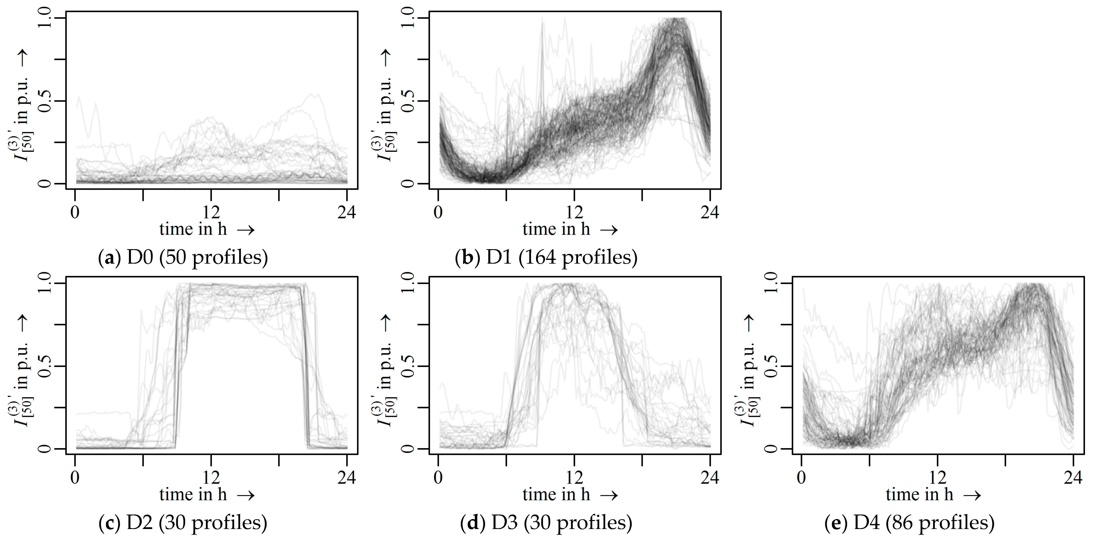
The resulting groups of the clustering process were assigned to one of the classes, D0 to D4, which are displayed in
Figure 5. The displayed profiles are used to illustrate the definition of the five classes that were used for the classification process.
Class D0: Daily time series without distinctive daily cycles, almost non-existent or no harmonic emission at all (c.f.
Figure 5a) were categorized as class D0. Examples are the emission profiles of office areas (c.f.
Figure 2a) and the electronic markets (c.f.
Figure 3a) for non-working or closed days.
Class D1: The daily time series in class D1 (c.f.
Figure 5b) have increasing emission levels of harmonic currents until the evening hours (around 8 o’clock) and decreasing levels during nighttime. The shape of the emission profiles is typical for consumer configurations in residential areas. Differences between single- or multi-family houses were not present for the analyzed LV networks.
Class D2: The emission profiles of class D2 can be distinguished into two time intervals. For the example of the electronic market (c.f.
Figure 5c) the two intervals were within the opening hours (high emission levels) and the closing hours (low emission levels). The transition between the two time intervals is usually within a short time frame, of less than one hour, and is strictly related to the opening hours.
Class D3: The class D3 (c.f.
Figure 5d) represents emission profiles that are typical for consumer configurations like office areas. The emission levels can be divided into two time intervals. In comparison to class D2 the transition between the two intervals has a longer duration of multiple hours. This might occur due to different working hours within different offices.
Class D4: The emission profiles of class D4 (c.f.
Figure 5e) are usually represented by measurements in mixed areas which are a combination of, for example, residential and office areas. This results in the typical “evening peak” of emission levels, as in class D1, and the time interval of distinctive emission levels during working hours, as in class D3.
5. Classification of Harmonic Emissions Profiles
The definition and the categorization of the 360 emission profiles for the 3rd harmonic current (c.f.
Figure 5) were required for the development of the classification system for harmonic emission profiles using machine learning methods. The given requirements of pre-known classes allow for the use of supervised learning algorithms, such as binary tree structure classifiers, in combination with support vector machines (SVM) [
25]. SVMs have been proven to be suitable in terms of classification rate and adaptiveness to the given classification problems. SVMs have been successfully applied for large amounts of data [
26] and a wide range of applications in power systems, from energy theft detection [
27], islanding, and grid fault detection [
28] to classification of power quality disturbances [
29,
30,
31,
32,
33]. For continuous PQ parameters, such as harmonics, the present applications rarely go beyond the generation of static reports and the comparison with respective limits. An automated classification system can support network operators with the identification of consumer configurations and the early detection of fundamental changes in the harmonic emission behavior at a particular site. This way it can extract valuable information about the PQ characteristics of a grid, which can serve as basis for further optimization of planning and operation in future grids.
5.1. Binary Tree Structure Classifier
The multi-class classification problem of five groups was divided into multiple two-class classifications using a binary tree structure classifier. The structure of the tree classifier was based on a top-down approach, and is displayed in
Figure 6.
The automated classification of emission profiles usually achieves better results if the easier classification problems are treated first [
34]. Therefore, the first two-class decision was applied between the class D0 and the classes (D1, D2, D3, D4). The classes (D1, D4) and (D2, D3) were divided in a second two-class decision, and were finally divided into D1 or D4 and D2 or D3 within two additional classification steps [
22].
5.2. Feature Selection
The two-class decisions require suitable features in order to distinguish between the different classes of emission profiles. The features are calculated for all emission profiles and the most efficient features for the four individual classifiers are selected.
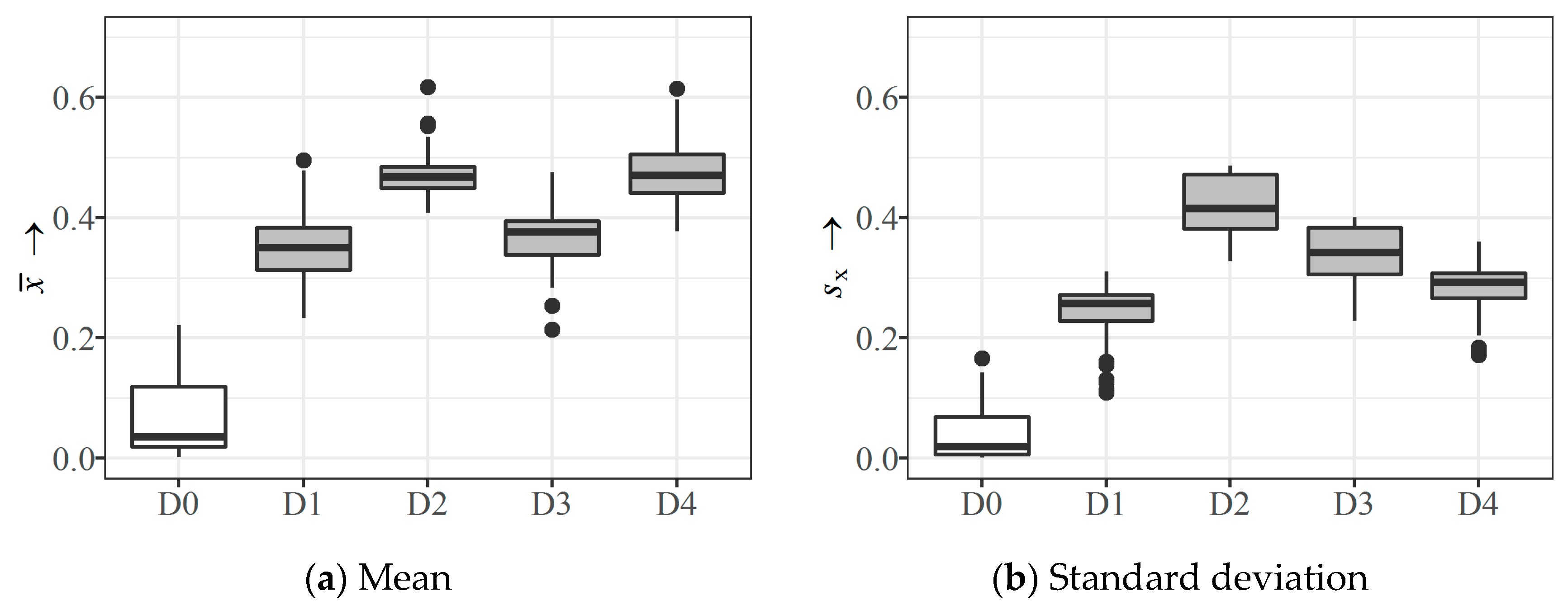
5.2.1. Features for Classifier SVM-1
The first classifier to distinguish between D0 and (D1, D2, D3, D4) uses the mean,
, and the standard deviation,
, of the emission profiles. Both features are displayed in
Figure 7 and show significantly lower values for class D0 in comparison to the remaining classes D1 to D4.
5.2.2. Features for Classifier SVM-2
The classifier SVM-2 uses two different features to distinguish between the classes (D1, D4) and (D2, D3). The mean of the emission profiles between 9 p.m. and 12 p.m. in the evening addresses the emission “peaks” in the evening hours for residential areas. The range between midnight and 3 a.m. in the morning highlights the higher variation of the emission in the morning hours for the classes D1 and D4.
5.2.3. Features for Classifier SVM-3
The separation of class D1 and class D4 is based on the mean between 9 a.m. in the morning and 3 p.m. in the afternoon, which is related to typical working hours in Germany. The 60th percentile is used as an additional feature.
5.2.4. Features for Classifier SVM-4
Classifier SVM-4 distinguishes between class D2 and class D3. The first feature is based on the mean between 5 p.m. and 8 p.m. in the evening, in order to highlight the difference between the transitions of the time intervals with and without higher levels of emission for the two classes. The 60th percentile is also used as an additional feature.
5.3. Implementation of Support Vector Machines
As a last step after definition of the five classes for the emission profiles and selection of features for their separation, the actual classifiers had to be implemented. Therefore, support vector machines (SVM) with a radial basis function kernel (RBF kernel) were proven as a suitable choice [
22]. The SVM as a classifier is robust against typical problems like overfitting, which results in higher classification rates [
34]. The computational effort is usually lower in comparison to other methods like Bayes classifications [
35].
The basic idea of SVMs is to construct a hyperplane within the feature space in order to divide the emission profiles according to their known classes. The hyperplane aims to separate two classes with a clear margin that is as wide as possible. The class of new emission profiles, which are mapped into the same feature space, are predicted based on which side of the hyperplane they are allocated. The regularisation parameter,
, that strongly affects the resulting hyperplane is user specified [
36].
5.3.1. Radial Basis Kernel Function
One of the main advantages of SVMs is the use of kernel functions, which allow for the classification of non-linear separable data sets. The reason for such a mapping is that it is more likely to obtain a linearly separable region in a higher dimensional space than a lower dimensional space [
35]. This can be achieved with the RBF kernel function:
The user-specified kernel parameter, , is a second parameter that strongly affects the resulting hyperplane and the respective classification results.
5.3.2. Determination of Optimal Parameters
A selection of optimal parameters for the regularisation parameter,
C, and the kernel parameter,
, is required before the application of SVMs with a RBF kernel. A simple grid search, using k-fold cross-validation to find the two best parameters (C,
) within a wide enough parameter range [
37], is applied to each of the SVMs. The two parameter ranges
and
are suitable for the given classification problem.
A cross-validation is applied for each combination of (C,
), dividing the training set into
k equally sized subgroups. The training is applied
k-times, whereas each time one group is tested against the remaining groups to determine the error rate. The result of the grid search for optimal parameters (C,
) of the classifier SVM-1 is displayed in
Figure 8.
The training results of SVM-1 with the optimal parameters in
Figure 9a had a classification rate of 96.3%, with one misclassification.
Selecting suboptimal parameters may result in perfect classification rates of 100% for the training, as displayed in
Figure 9b. Future classifications will very likely lead to many misclassifications due to the overfitting to the training samples.
6. Classification of Harmonic Emission Profiles
The evaluation of the classification was applied using the 360 emission profiles from
Figure 5. The emission profiles were randomly divided into a training and test samples. According to [
38] split ratios of 50:50 to 70:30 mostly give good results, whereas splits of 90:10 are recommended for a very small sample size. The training set should be large enough in order to maintain the generalization abilities of the classifiers. A division into 50% for the training samples and 50% for the test samples leads to good results for the given data set.
6.1. Performance Evaluation
The resulting numbers for a random split of the emission profiles per class are presented in
Table 1. The optimal parameters for the regularisation parameter,
C, and the kernel parameter,
, were determined for each of the classifiers SVM-
i,
using the training samples.
The emission profiles of
Figure 5 were used as a reference for the classification in order to identify misclassifications. The classification results for the training process of the classification system are listed in
Table 2.
An average false alarm rate of 4.6% was achieved for the separate classes, which equals about two misclassified emission profiles per class. The actual evaluation of the classification system was determined by classifying the “unknown” test samples. The results for the classification of the test samples are presented in
Table 3. A classification rate of 95.5%, similar to the training results, was obtained.
6.2. Robustness of Performance
The process of randomly splitting into training and test samples was repeated 100 times in order to evaluate the robustness of the classification system independently from one specific split, as presented in
Table 1. The average and per class classification rates are represented as box whisker plots in
Figure 10, and separately for the training samples and the test samples.
The median of the average classification rates was 97.0% for the training samples and 92.3% for the test samples. The different classification results varied for different splits. Nevertheless, the lowest classification rates per class did not fall below 72%.
7. Measure of Misclassification
The definition of five classes of emission profiles may result in misclassifications for completely different profiles. A new but not implemented emission profile is assigned to one of the defined classes even if it does not fully match. A simple measure of misclassification was defined in order to overcome these inherent shortcomings [
22]. The measure of misclassification,
, is based on the average distance between all emission profiles in one group, compared to the distance of the new emission profile.
The Euclidian distance
was used to calculate the dissimilarity between two emission profiles
and
within one group. The average distance between one emission profile and all others profiles of one group can be calculated as follows:
and results for
emission profiles within one group in
average distances. The 25th percentile
and the 75th percentile
are calculated. A newly classified emission profile, y, can be defined as an outlier, similarly to the definition of the box-whisker plots in [
39]:
The measure of misclassification for newly quantified emission profiles is calculated as follows:
High values of
are used as an indicator showing that newly classified emission profiles strongly differ from the training samples of the assigned class. The measures of misclassification are exemplarily presented in
Figure 11a,c for test samples of the classes D1 and D2. Two assignments with
and one assignment with
indicate that the emission profiles differed from the training samples of the respective classes. The actual emission profiles, which are displayed in
Figure 11b,d, emphasized that the higher the measure, the more likely the misclassification of the classified emission profile.
Nevertheless, emission profiles should be manually reviewed by the user of the classification system. Additional measurements or the definition of a new class of emission profiles may be needed, depending on the individual results.
8. Conclusions
The emission of harmonic currents in public LV networks is mainly influenced by the consumer and generating configuration. Especially the harmonic emission of certain consumer configurations, such as commercial areas, is strongly related to the typical usage of the connected equipment. The analysis of weekly and daily time series of harmonic currents confirms that the three different day types, Mondays to Fridays, Saturdays, and Sundays and Holidays, are represented. The harmonic emission behaviour for these day types is very consistent and differs according to the typical German consumer configurations residential, offices, commercial, and mixed areas.
The harmonic emission behaviour was used for the development of a classification system in order to identify a probable consumer configuration based on the measurement of their respective harmonic currents, especially the 3rd harmonic current. A binary decision tree using support vector machines was used for the classification system, which requires training for the actual application. The features to distinguish between the different classes were introduced for each of the four SVMs. The measured emission profiles were grouped accordingly to the predefined classes. The performance evaluation was highlighted for 360 emission profiles, which were split into 50% for the training set and 50% for the test set. The results showed an average classification rate of at least 95%. The random split into training and test samples was repeated one hundred times in order to evaluate the robustness of the classification, and revealed similar classification rates for the training and test processes.
The emission profiles used for the training process strongly influenced the classification results. A measure of misclassification was introduced in order to enable the identification of misclassified emission profiles by the user of the classification system. It can be used as an indicator for emission profiles that differ strongly from the assigned profile class respective to their associated training samples. A manual review of misclassified profiles enables the user to identify unusual emission behaviour of specific measurement sites, i.e., anomaly detection.
The automatic identification of consumer configurations based on their harmonic emission is a first contribution towards more automated analysis of large data quantities and to keeping the routine assessment of PQ levels efficient.
Author Contributions
Conceptualization, M.D. and I.Y.-H.G.; methodology, M.D. and I.Y.-H.G.; software, M.D.; validation, M.D.; formal analysis, M.D.; investigation, M.D.; resources, P.S.; data curation, M.D. and J.M.; writing—original draft preparation, M.D.; writing—review and editing, M.D., I.Y.-H.G. and J.M.; visualization, M.D; project administration, P.S.; funding acquisition, P.S. All authors have read and agreed to the published version of the manuscript.
Funding
This research was funded by the German Research Foundation (Deutsche Forschungsgemeinschaft—DFG), grant number SCHE 571/8-2.
Institutional Review Board Statement
Not applicable.
Informed Consent Statement
Not applicable.
Data Availability Statement
Restrictions apply to the availability of these data. Data was obtained from measurement campaigns with two German distribution system operators and are available with their permission.
Conflicts of Interest
The authors declare no conflict of interest.
References
- Santoso, S.; McGranaghan, M.F.; Dugan, R.C.; Beaty, H.W. Electrical Power Systems Quality, 3rd ed.; McGraw-Hill Professional: New York, NY, USA, 2012. [Google Scholar]
- Arrillaga, J.; Watson, N.R. Power System Harmonics; Wiley: Hoboken, NJ, USA, 2003. [Google Scholar]
- Yazdani-Asrami, M.; Mirzaie, M.; Akmal, A.A.S. No-load loss calculation of distribution transformers supplied by nonsinusoidal voltage using three-dimensional finite element analysis. Energy 2013, 50, 205–219. [Google Scholar] [CrossRef]
- Zavoda, F. The key role of intelligent electronic devices (IED) in advanced Distribution Automation (ADA). In Proceedings of the 2008 China International Conference on Electricity Distribution, Guangzhou, China, 10–13 December 2008; pp. 1–7. [Google Scholar]
- Elphick, S.; Ciufo, P.; Drury, G.; Smith, V.; Perera, S.; Gosbell, V. Large Scale Proactive Power-Quality Monitoring: An Example from Australia. IEEE Trans. Power Deliv. 2017, 32, 881–889. [Google Scholar] [CrossRef]
- Kilter, J.; Elphick, S.; Meyer, J.; Milanovic, J.V. Guidelines for Power quality monitoring—Results from CIGRE/CIRED JWG C4.112. In Proceedings of the 2014 16th International Conference on Harmonics and Quality of Power (ICHQP), Bucharest, Romania, 25–28 May 2014; pp. 703–707. [Google Scholar] [CrossRef]
- Meyer, J.; Schegner, P.; Eberl, G. Increasing the reliability of indices for power quality assessment in distribution networks. In Proceedings of the 2008 13th International Conference on Harmonics and Quality of Power, Wollongong, NSW, Australia, 28 September–1 October 2008; pp. 1–6. [Google Scholar]
- Domagk, M.; Meyer, J.; Schegner, P. Seasonal variations in long-term measurements of power quality parameters. In Proceedings of the 2015 IEEE Eindhoven PowerTech, Eindhoven, The Netherlands, 29 June–2 July 2015; pp. 1–6. [Google Scholar]
- Domagk, M.; Meyer, J.; Schegner, P. Characterization of public low voltage grids by clustering time series of power quality parameters. In Proceedings of the 12th International Conference, Istanbul, Turkey, 10–14 June 2012; pp. 558–563. [Google Scholar]
- Salles, D.; Jiang, C.; Xu, W.; Freitas, W.; Mazin, H.E. Assessing the Collective Harmonic Impact of Modern Residential Loads—Part I: Methodology. IEEE Trans. Power Deliv. 2012, 27, 1937–1946. [Google Scholar] [CrossRef]
- Devarapalli, H.P.; Dhanikonda, V.S.S.S.S.; Gunturi, S.B. Non-Intrusive Identification of Load Patterns in Smart Homes Using Percentage Total Harmonic Distortion. Energies 2020, 13, 4628. [Google Scholar] [CrossRef]
- Meyer, J.; Blanco, A.-M.; Domagk, M.; Schegner, P. Assessment of Prevailing Harmonic Current Emission in Public Low-Voltage Networks. IEEE Trans. Power Deliv. 2016, 32, 962–970. [Google Scholar] [CrossRef]
- Domagk, M.; Zyabkina, O.; Meyer, J.; Schegner, P. Trend identification in power quality measurements. In Proceedings of the 2015 Australasian Universities Power Engineering Conference (AUPEC), Wollongong, Australia, 7–30 September 2015; pp. 1–6. [Google Scholar]
- Gil-De-Castro, A.; Rönnberg, S.; Bollen, M.H.J.; Moreno-Munoz, A.; Pallares-Lopez, V. Harmonics from a domestic customer with different lamp technologies. In Proceedings of the 2012 IEEE 15th International Conference on Harmonics and Quality of Power, Hong Kong, China, 17–20 June 2012; pp. 585–590. [Google Scholar]
- Electromagnetic Compatibility (EMC)—Part 4-30: Testing and Measurement Techniques—Power Quality Measurement Methods; IEC: Geneva, Switzerland, 2015.
- Bodnar, R.; Otcenasova, A.; Regul’A, M.; Szabo, D. Measurement of harmonics in low-voltage network on the border between SVK and CZE. In Proceedings of the 2014 15th International Scientific Conference on Electric Power Engineering (EPE), Brno, Czech Republic, 2–14 May 2014; pp. 217–222. [Google Scholar]
- Kutt, L.; Saarijärvi, E.; Lehtonen, M.; Mõlder, H.; Vinnal, T. Harmonic load of residential distribution network Case study monitoring results. In Proceedings of the 2014 Electric Power Quality and Supply Reliability Conference (PQ), Rakvere, Estonia, 11–13 June 2014; pp. 93–98. [Google Scholar]
- Kouveliotis-Lysikatos, I.; Kotsampopoulos, P.; Hatziargyriou, N. Harmonic Study in LV networks with high penetration of PV systems. In Proceedings of the 2015 IEEE Eindhoven PowerTech, Eindhoven, The Netherlands, 29 June–2 July 2015; pp. 1–6. [Google Scholar]
- Zhou, K.-L.; Yang, S.-L.; Shen, C. A review of electric load classification in smart grid environment. Renew. Sustain. Energy Rev. 2013, 24, 103–110. [Google Scholar] [CrossRef]
- Chicco, G.; Ionel, O.-M.; Porumb, R. Electrical Load Pattern Grouping Based on Centroid Model with Ant Colony Clustering. IEEE Trans. Power Syst. 2012, 28, 1706–1715. [Google Scholar] [CrossRef]
- Jiang, Z.; Lin, R.; Yang, F. A Hybrid Machine Learning Model for Electricity Consumer Categorization Using Smart Meter Data. Energies 2018, 11, 2235. [Google Scholar] [CrossRef]
- Domagk, M. ‘Identifikation und Quantifizierung korrelativer Zusammenhänge zwischen elektrischer sowie klimatischer Umgebung und Elektroenergiequalität’. Ph.D. Thesis, Technische Universität Dresden, Dresden, Germany, 2015. [Google Scholar]
- Meier, C.H.; Adam, F.T.; Schieferdecker, B. Repräsentative VDEW-Lastprofile; VDEW: Frankfurt, Germany, 1999. [Google Scholar]
- Chakrabarti, S.; Neapolitan, R.E.; Pyle, D. Data Mining: Know It All; Elsevier Science: Amsterdam, The Netherlands, 2008. [Google Scholar]
- Lee, J.-S.; Oh, I.-S. Binary classification trees for multi-class classification problems. In Proceedings of the Seventh International Conference on Document Analysis and Recognition, Proceedings, Edinburgh, UK, 3–6 August 2003. [Google Scholar]
- Wu, J.; Yang, H. Linear Regression-Based Efficient SVM Learning for Large-Scale Classification. IEEE Trans. Neural Networks Learn. Syst. 2015, 26, 2357–2369. [Google Scholar] [CrossRef] [PubMed]
- Jindal, A.; Dua, A.; Kaur, K.; Singh, M.; Kumar, N.; Mishra, S. Decision Tree and SVM-Based Data Analytics for Theft Detection in Smart Grid. IEEE Trans. Ind. Inform. 2016, 12, 1005–1016. [Google Scholar] [CrossRef]
- Baghaee, H.R.; Mlakic, D.; Nikolovski, S.; Dragicevic, T.D. Support Vector Machine-Based Islanding and Grid Fault Detection in Active Distribution Networks. IEEE J. Emerg. Sel. Top. Power Electron. 2019, 8, 2385–2403. [Google Scholar] [CrossRef]
- Naderian, S.; Salemnia, A. Method for classification of PQ events based on discrete Gabor transform with FIR window and T2FK-based SVM and its experimental verification. IET Gener. Transm. Distrib. 2017, 11, 133–141. [Google Scholar] [CrossRef]
- Thirumala, K.; Prasad, M.S.; Jain, T.; Umarikar, A.C. Tunable-Q Wavelet Transform and Dual Multiclass SVM for Online Automatic Detection of Power Quality Disturbances. IEEE Trans. Smart Grid 2018, 9, 3018–3028. [Google Scholar] [CrossRef]
- Sha, H.; Mei, F.; Zhang, C.; Pan, Y.; Zheng, J. Identification Method for Voltage Sags Based on K-means-Singular Value Decomposition and Least Squares Support Vector Machine. Energies 2019, 12, 1137. [Google Scholar] [CrossRef]
- Bravo-Rodríguez, J.C.; Torres, F.J.; Borrás, M.D. Hybrid Machine Learning Models for Classifying Power Quality Disturbances: A Comparative Study. Energies 2020, 13, 2761. [Google Scholar] [CrossRef]
- Tang, Q.; Qiu, W.; Zhou, Y. Classification of Complex Power Quality Disturbances Using Optimized S-Transform and Kernel SVM. IEEE Trans. Ind. Electron. 2019, 67, 9715–9723. [Google Scholar] [CrossRef]
- Duda, R.O.; Hart, P.E.; Stork, D.G. Pattern Classification, 2nd ed.; John Wiley & Sons: New York, NY, USA, 2012. [Google Scholar]
- Bollen, M.H.J.; Gu, I.Y.-H. Signal Processing of Power Quality Disturbances; Wiley: Hoboken, NJ, USA, 2006. [Google Scholar]
- Abe, S. Support Vector Machines for Pattern Classification; Springer Science and Business Media LLC: Berlin/Heidelberg, Germany, 2010. [Google Scholar]
- Chang, C.-C.; Lin, C.-J. LIBSVM. ACM Trans. Intell. Syst. Technol. 2011, 2, 1–27. [Google Scholar] [CrossRef]
- Athimethphat, M.; Lerteerawong, B. Binary classification tree for multiclass classification with observation-based clustering. In Proceedings of the 2012 9th International Conference on Electrical Engineering/Electronics, Computer, Telecommunications and Information Technology, Phetchaburi, Thailand, 16–18 May 2012. [Google Scholar] [CrossRef]
- Tukey, J.W. Exploratory Data Analysis; Addison-Wesley: Boston, MA, USA, 1977. [Google Scholar]
Figure 1.
Classification of variation types and major impact factors in public LV networks [
8].
Figure 1.
Classification of variation types and major impact factors in public LV networks [
8].
Figure 2.
Profile of the 3rd harmonic current for an office building; median (red), 5th and 95th percentile (blue), daily time series (grey); aggregation interval: 10 min; measurement duration: 320 days from January to December 2012.
Figure 2.
Profile of the 3rd harmonic current for an office building; median (red), 5th and 95th percentile (blue), daily time series (grey); aggregation interval: 10 min; measurement duration: 320 days from January to December 2012.
Figure 3.
Profile of the 3rd harmonic current for an electronic market; median (red), 5th and 95th percentile (blue), daily time series (grey); aggregation interval: 10 min; measurement duration: 353 days from January to December 2012.
Figure 3.
Profile of the 3rd harmonic current for an electronic market; median (red), 5th and 95th percentile (blue), daily time series (grey); aggregation interval: 10 min; measurement duration: 353 days from January to December 2012.
Figure 4.
Example for typical emission profiles of the 3rd harmonic order for different consumer configurations: residential (RES), commercial (COM), office (OFF), and mixed (MIX) areas; min-max scaled 50th percentile time series for different day types: working days (G1), Saturdays (G2), and Sundays/holidays (G3); phase L1; aggregation interval: 10 min.
Figure 5.
Classes of emission profiles for the 3rd harmonic current; min–max normalized 50th percentile time series for 40 measurements in LV grids within three groups: working days, Saturdays, and Sundays/holidays for all phases L1 to L3.
Figure 5.
Classes of emission profiles for the 3rd harmonic current; min–max normalized 50th percentile time series for 40 measurements in LV grids within three groups: working days, Saturdays, and Sundays/holidays for all phases L1 to L3.
Figure 6.
Binary tree structure classifier for emission profiles.
Figure 6.
Binary tree structure classifier for emission profiles.
Figure 7.
Features of the emission profiles for the first classifier support vector machine (SVM)-1 to distinguish class D0 and classes (D1, D2, D3, D4).
Figure 7.
Features of the emission profiles for the first classifier support vector machine (SVM)-1 to distinguish class D0 and classes (D1, D2, D3, D4).
Figure 8.
Grid search for the optimal parameters of the classifier SVM-1 using a cross-validation with 10 subgroups (k = 1); error rate in p.u.
Figure 8.
Grid search for the optimal parameters of the classifier SVM-1 using a cross-validation with 10 subgroups (k = 1); error rate in p.u.
Figure 9.
Training for the classifier SVM-1, with the resulting hyperplane using optimal parameters (a), and suboptimal parameters (b).
Figure 9.
Training for the classifier SVM-1, with the resulting hyperplane using optimal parameters (a), and suboptimal parameters (b).
Figure 10.
Robustness for the classification of 360 emission profiles; 100 repetitions, with random splits into 50% training samples and 50% test samples; box whisker plots of average and per class classification rates for training samples (white) and test samples (grey).
Figure 10.
Robustness for the classification of 360 emission profiles; 100 repetitions, with random splits into 50% training samples and 50% test samples; box whisker plots of average and per class classification rates for training samples (white) and test samples (grey).
Figure 11.
Measures of misclassification for the classes D1 and D2, and emission profiles of training samples (grey), and test samples (blue/red).
Figure 11.
Measures of misclassification for the classes D1 and D2, and emission profiles of training samples (grey), and test samples (blue/red).
Table 1.
Number of emission profiles per class using a random separation into training samples and test samples.
Table 1.
Number of emission profiles per class using a random separation into training samples and test samples.
| Class | D0 | D1 | D2 | D3 | D4 |
|---|
| Training samples | 27 | 85 | 15 | 15 | 38 |
| Test samples | 23 | 79 | 15 | 15 | 48 |
Table 2.
Classification results for the training samples of
Table 1.
Table 2.
Classification results for the training samples of
Table 1.
| Class | D0 | D1 | D2 | D3 | D4 | Average |
|---|
Number of
misclassifications | 1 | 4 | 0 | 1 | 3 | 1.8 |
| Classification rate in % | 96.3 | 95.3 | 100 | 93.3 | 92.1 | 95.4 |
Table 3.
Classification results for the test samples of
Table 1.
Table 3.
Classification results for the test samples of
Table 1.
| Class | D0 | D1 | D2 | D3 | D4 | Average |
|---|
Number of
misclassifications | 0 | 4 | 1 | 1 | 2 | 1.6 |
| Classification rate in % | 100 | 94.9 | 93.3 | 93.3 | 95.8 | 95.5 |
| Publisher’s Note: MDPI stays neutral with regard to jurisdictional claims in published maps and institutional affiliations. |
© 2021 by the authors. Licensee MDPI, Basel, Switzerland. This article is an open access article distributed under the terms and conditions of the Creative Commons Attribution (CC BY) license (https://creativecommons.org/licenses/by/4.0/).


