Increasing Wind Turbine Drivetrain Bearing Vibration Monitoring Detectability Using an Artificial Neural Network Implementation

Abstract

The highest costs due to premature failures in wind turbine drivetrains are related to defects in the gearbox, with bearing failures being overrepresented. Vibration monitoring has been identified as the primary tool to detect and diagnose these types of failures. However, late or no signs of the failures are still being reported. Artificial neural networks (ANNs) has been shown to favourably be used as a classifier of bearing failures to increase the detection and diagnosis performance, which requires labelled data when training for all types of considered failures. However, less work has been done with an ANN used to create descriptive functions of the vibration and turbine operation data relationship and thereby negating inherent variance in the vibration data and increasing the detectability when a defect appears. Therefore, this study utilizes the relationship between the rotational speed recorded during a vibration measurement and the calculated condition indicator values of specific bearing failures in three wind turbine gearbox failures. An ANN establishes a function between the rotational speed and condition indicator values with healthy training data collected before the failure occurred. Thereafter, whole datasets leading up to the changing of the gearboxes is used to predict the condition indicator values without the failure influence. The difference between the predicted and true values show an increased sensitivity of the detection in two cases of gearbox output shaft bearing failures as well as indicating a planet bearing failure which with the previous data had gone undetected.

1. Introduction

Wind power is one of the main growing energy generating sectors, which in 2019 saw its second-largest increase in capacity with 60.4 GW, making the total 651 GW [1]. However, wind turbines experience a large number of premature failures, with the most costly ones being in the drivetrain. Further, the gearbox is the highest contribution to these costs, partly due to the long downtime associated with these failures and e.g., the price of a new 2 MW gearbox being as high as 400 k€ [2]. Out of these gearbox failures, the bearings are over-represented compared to the gears by a factor of 76% to 17% [3]. To efficiently combat the costs associated with the drivetrain failures, online condition monitoring has become the main method to ensure the health of the bearings and gears [4]. Monitoring by vibration measurements is employed as it can differentiate vibrations from bearing and gear components in a sub-system, and thereby can at an early stage effectively diagnose a detected failure to its origin component. Thereby, the developing failure can be monitored live, maintenance planning start at an earlier date limiting the downtime and actions in operation of the turbine, such as limiting the power output for a period of time, can be taken to reduce the cost of the failure.

The vibration monitoring is normally done by trend values calculated from consecutive measurements, as well as specific peaks in the frequency domain correlated to different bearing components experiencing defects or gear contacts. Base values of these indicators first need to be established before deviations in new data points from this trend can indicate a defect being present. This procedure is often done by experts needing to make decisions in small ocular differences in the data, based on experience. Thereby, an as sensitive monitoring and signal analysis solution as possible is preferable to increase the certainty of maintenance decisions.

Lately, much research has been done with machine learning techniques to more efficiently detect, diagnose and predict bearing failures. Most often, techniques such as artificial neural networks (ANNs) [5,6,7,8,9], is used as it can design a descriptive function from complex observations [10], or support vector machines (SVMs) [11,12,13], used for its high generalization ability [14], are implemented as classifiers if data points can be considered healthy or a fault is present, and in extension which bearing component has a defect. Moreover, other techniques such as the random forest classification technique have been implemented in rolling bearing failure detection and diagnosis to attempt to fully replace the need for an expert analysis of the data and to better handle a large number of input variables [15,16]. However, such techniques and the multitude of extensions to the base neural networks and SVM techniques introduce their own set of complexities in generalizing an implementation to perform on each individual case and individual machine. Therefore, value can be gained by introducing a machine learning implementation as a step in the current condition monitoring methodology to increase the interpretable signs of deteriorating bearings, which the more complex and advanced techniques are not designed for. Additionally, labelled data, where the presence of a defect cannot be argued, are often needed for training the algorithms, which outside of a simulated or lab environment is difficult to acquire and had up to 2015 largely been overlooked [17]. Thereby, an implementation that does not require labelled data has an advantage when applied to existing wind turbine vibration field data. However, studies into various condition monitoring techniques using vibration field data as opposed to simulated or test rig data are starting to become more popular. In de Azevedo’s bearing condition monitoring review from 2016 less than 8% were using field data while in Liu’s review from 2020, this had increased to 40%. A number of machine learning techniques were employed in some of these studies, but only one used an ANN [18,19].

Work using wind turbine field data has also been focused on using data from the turbine Supervisory Control And Data Acquisition (SCADA) system in ANNs to detect defects [20,21,22]. Here, parameters such as the wind speed, blade pitch angle, drivetrain component temperatures and generated power can be used to find abnormal behaviour in the turbines state and operation which could indicate a defect being present. Keeping in mind that among the typical monitoring techniques, vibration monitoring can detect defect at an earlier stage compared to lubrication and temperature monitoring, this would still be used as the main indicator for a defect being present. However, the integration between the SCADA and condition monitoring systems data sources is often non-existent [23]. Therefore, a lot of hands-on work is needed in each individual case to prepare the data which greatly hampers a machine learning solution to be widely introduced in wind turbine monitoring. An implementation that at most only requires the input of operational data which is stored as metadata to the vibration measurements, where the integration of the two data types exists, is therefore of interest. A first step to introduce a machine learning solution can be to make use of the few operational parameters which exist in the condition monitoring system and find abnormal behaviour to correlate to the presence of a defect. Another important advantage to take into consideration with such a solution is the need to obtain labelled data only when healthy for the learning period, instead of when used as a classifier where both healthy data and labelled data during all types of failures are needed.

This study utilizes vibration monitoring results leading up to three different wind turbine gearbox bearing failures. More specifically condition indicator values for the specific failures, providing the detection and diagnosis, is used. The three failures consist of two gearbox output shaft bearing failures which are clearly detectable, and one planet bearing failure from the second planetary gear stage which is problematic to detect and diagnose. The novelty of this study is showing the implementation of an ANN regression solution, chosen for its highly adaptable ability to quickly design functions from complex observations, between condition indicator results when the healthy and rotational speed of the gearbox output shaft, an associated measurement to the vibration measurements within the condition monitoring database, enabling an implementation without the need for labelled data. Thereby, the ANN implementation can be used to predict the condition indicator value as it should be during normal operation and when compared to true values with developing defects affecting the system, exhibit this difference as a more sensitive detection method than purely the condition indicator values themselves. The goal of this study is then to improve the sensitivity of the condition monitoring system and highlight signs of a defect that might not be possible by pure ocular observations of the condition indicator trends.

In Section 2, the ANN implementation methodology is presented with summarized failure case information and condition indicator results. The results are presented and discussed in Section 3 and conclusions in Section 4.

2. Method

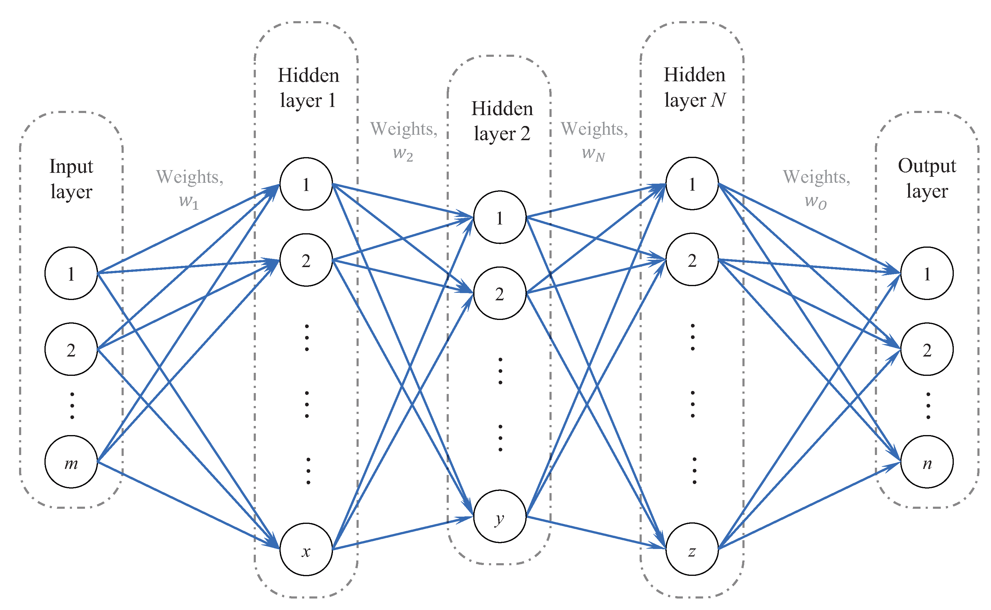
2.1. Artificial Neural Networks

The general ANN structure consists of three components denominated as layers, two “visible” layers being the known input layer to the network and the following output layer, and between these are either a singular or a multitude of hidden layers. These layers consist of a number of neurons each, with the input and output layers corresponding to the input size and the number of neurons in the hidden layers are chosen when setting up the network. Additionally, each neuron of one layer is connected to all neurons in the following layer. As the input is passed through the network, weights between each neuron calculate the output. These weights are initialized with random values and are in the training phase calibrated by iteratively minimizing the error between the output and the known target value through the backpropagation algorithm [24]. A schematic structure with N hidden layers can be seen in Figure 1.

2.2. Bearing Failure Cases

From three bearing failure cases, datasets of stored vibration measurements from the condition monitoring system databases were extracted covering different frequency ranges and measurement lengths. These datasets were processed with the enveloping technique where bandpass filtering and rectifying extracts the repetition frequency of impact resonances yielding an early detection of the defect in a bearing [25], and fast Fourier transform (FFT). Thereafter, condition indicator (CI) values for each failing bearing was constructed by a summation of three characteristic bearing defect frequency harmonics, and the failure progression could be analysed. The characteristic bearing defect frequency is calculated by multiplying the bearing shaft rotational speed and a relation between the bearing dimensions [26]. As it was on the inner ring of the bearings which experienced the defects, the ball pass frequency of the outer inner ring (BPFI) was used. This is calculated as:

$$BPFI=\frac{f{n}_i}{2}\left(1+\frac{D}{d_m}cos\left(\alpha \right)\right)$$

(1)

where f is the relative rotational frequency between the raceways, $n_i$ number of rolling elements, D rolling element diameter, $d_m$ pitch diameter, and $\alpha$ is the contact angle. Additionally, as the defects are mounted on rotating components, shaft speed sidebands will appear on each side of the BPFI harmonics. Three harmonics of the shaft speed sidebands on each BPFI harmonic were also used when calculating the CI-values, as:

$$C{I}_n=\sqrt{{\displaystyle \sum _{i=1}^{k=3}\sum _{j=1}^{l=\pm 3}{p}_{i,j}^2}}.$$

(2)

Here, $p_{i,j}$ is the specific peak acceleration amplitude level of $k=3$ fault frequency harmonics and $l=3$ shaft speed sideband harmonics where these theoretically should exist. An alternative method to convert the enveloped vibration measurements into the frequency domain which has previously shown to yield a higher CI-value increase, and in some cases at an earlier stage, is the wavelet packet transform (WPT). More information into this implementation and how it compares to the FFT, which is the standardized method in wind turbine drivetrain bearing monitoring to convert the enveloped measurements into the frequency domain, can be found in a previous study by the authors [27]. CI-values can therefore be calculated from two different spectra per measurement and trended over time. Henceforth, to differentiate between the two sets of CI-values these are denominated enveloped WPT and enveloped FFT CI-values.

The three bearing failure cases consists of two gearbox output shaft bearing failures, cases 1 and 3, and one planet bearing failure, case 2. For all cases, defects appeared on the inner raceways. Note: case 1 is partially reproduced results from [27]. The relevant failure case information is compiled in

Table 1. Bearing, damage and measurement information for each failure case.

Failure Case	1	2	3
Bearing	Output	Pl.2 Planet	Output
position	shaft		shaft
Bearing	SKF	SKF	SKF
designation	NU2230E	RN2238	32236J2
Damage	Inner ring	Inner ring	Inner ring
	spalling	spalling and flaking	spalling
Meas. type	Time sync	Time sync	Time sync and enveloped
Meas. time and	1.28 s, 0–5 kHz	6.4 s, 0–1 kHz	1.28 s, 0–5 kHz,
freq. range			32 rev, 0–10 kHz
Envelope filters	0.5–6.4 kHz,	0.2–1 kHz,	0.5–6.4 kHz, 0.2 kHz
	0.2 kHz	0.2 kHz	0.5–10 kHz, 0.5 kHz
Dataset size	562	1377	2102 and 754

. The specific envelope filters were determined to replicate the set filters in the vibration measurement systems mounted in the wind turbine drivetrains, as was the case in the authors previous study [27]. Comparative results between the enveloped FFT and the enveloped WPT CI-values for failure cases 1 and 2 can be seen in Figure 2a,b respectively with the enveloped FFT CI-values in blue and enveloped WPT CI-values in black trended over measurement number in the dataset as a parameter of time.

For the gearbox output shaft bearing failure in case 1 show an increase of the normalized, by z-score using the first 20 measurements as a healthy reference, CI-values as the defect has appeared. The enveloped WPT CI-value results can both yield a higher as well as an earlier increase, which is important for the monitoring to be as sensitive as possible. For the planet bearing failure in case 2 however, no apparent increase of the CI-values can be seen. A small difference can be seen in the last 200 measurements where the spread has decreased. However, these measurements have consistently been taken during high rotational speeds compared to earlier in the dataset and cannot be attributed to the present defect with any high degree of certainty. For failure case 3, enveloped FFT CI-values from 1.28 s long measurements and with a frequency range of 0–5 kHz were compared to CI-values extracted directly from the database from in-system enveloped measurements where the frequency range was extended to 0–10 kHz and the measurement time was taken over 32 revolutions of the gearbox output shaft, between 1.5 and 2.75 s. This type of in-system enveloped measurement is generally not stored in the databases and cannot, therefore, be used in a post-failure investigation. This comparison can be seen in failure case 3 in Figure 3 with the 0–5 kHz CI-values in blue in the top graph and 0–10 kHz in red in the bottom graph.

Additionally, since the number of CI-values for each frequency range differs, each CI-value is trended with respect to the number of days from the start of the dataset. The resonance frequencies demodulated by the enveloping technique primarily exist above the 5 kHz max frequency range of the extracted measurements until the last days of the dataset time period. Therefore, the 0–10 kHz CI-values can indicate the defect at a much earlier date.

2.3. Data Pattern and Filtration

An example of the relationship between the rotational speed measurement of the gearbox output shaft and the calculated CI-values, before normalization, can be seen in Figure 4a where the enveloped FFT CI-value results before the defect develops in failure 1 are used. Included in this is CI-values from measurements taken under two different scenarios. As this specific type of turbine has been at standstill, it will need to reach a rotational speed above 880 rpm before the generator starts to produce. Thereafter, it can be allowed to decrease in rotational speed to roughly 750 rpm before the generator stops producing again. However, the limitations set on the monitoring system regarding when to store a vibration measurement does not take this into account. Instead, limits have been set on the rotational speed between 700–1300 rpm and the rotational speed variance during the measurement to no more than 30 rpm. Thereby, measurements will exist in the database where the resistance in the drivetrain from the generator will be much lower, and this will in turn affect the general amplitude level of the vibration spectra. Additionally, the three measurements taken during the highest rotational speed of the gearbox output shaft do not follow the established pattern. It was shown that the variance in speed as these measurements was relatively high at 13.7, 8.96 and 17.8 rpm respectively.

Therefore, another input data filtering operation was added where measurements taken with more variance in rotational speed of 8 rpm were eliminated from the dataset. In Figure 4b, the enveloped FFT CI-values dependent on the variance in rotational speed during the measurement is presented. Therefore, the invalid CI-values, seen in red when taken during generator not producing and in black respect to the high variance in rotational speed in Figure 4a,b, has been identified in the failure case 1 and 3 datasets and removed, leaving the valid CI-values in blue. For the planet bearing failure in failure case 2 however, the variance in rotational speed of that bearing was only at most 4.3 rpm due to the downshift in rotational speed compared to the tachometer measurement position. Thereby, no further data elimination with respect to rotational speed variance was made in that case.

2.4. Procedure

After this, the first 300 CI-values with accompanying rotational speed value in each dataset was chosen as training data for each respective case. Two sets of ANNs, one for the enveloped FFT CI-value results and one for the enveloped WPT CI value results, were trained for each failure case. These had three hidden layers with 64, 8 and 64 neurons respectively. In the early stage of this investigation, a multitude of structures concerning the number of hidden layers and neurons, were tested. While it was shown that a simpler one or two hidden layer structure could produce comparable prediction results, as long as the number of neurons was sufficiently high, this three-layer structure was shown to yield more stable and repeatable results without any decrease in performance. Therefore, it was decided to use this structure for each failure case. The rotational speed measurements were used as input and CI-values before normalization as output. The ANNs were set up in Matlab using the fitnet function and trained using the Levenberg–Marquardt algorithm for optimal computational speed. By using these trained ANNs to predict the CI-values for the remaining measurements in the datasets, the effect of the defect on the measurements is separated from the inherent rotational speed dependant, CI-value variance. The difference, $d_n$ between the true CI-values, $C{I}_n$, and the predicted values, $p_n$, were calculated for each measurement, n, in the datasets by

$$d_n=\sqrt{{\left(C{I}_n-p_n\right)}^2}.$$

(3)

Z-score normalization was used to be able to compare the differentiation results between the true and predicted CI-values between the two signal analysis methods, and the detectability performance of the true CI-values by themselves. The normalization of one value of the difference between the true and predicted values is calculated by

$$Z_n=\frac{d_n-\mu \left(d_{1,2,\dots ,20}\right)}{\sigma \left(d_{1,2,\dots ,20}\right)},$$

(4)

where the $\mu$ and $\sigma$ values are calculated from the first 20 values.

3. Results and Discussion

3.1. Failure Case 1 Results

In Figure 5a, the ANN’s predicted enveloped FFT CI-values from failure case 1 can be seen together with the comparison with the true values and the normalized difference between them, before data filtration with respect to rotational speed variance.

At the top graph, the ANN’s predicted CI-values are seen in red and closely followed the true values, in blue, until the defect appeared except for three distinct peaks. These three predicted values coincided with the three mentioned measurements in Section 2.3 which were taken during a high rotational speed and large variance. The ANN learned that such a high rotational speed should coincide with a high CI-value but failed to take into account the flattening effect of the spectrum when the variance in rotational speed was high. Thereby, the calculated difference, using Equation (3) and seen in normalized form by Equation (4) in the bottom graph of Figure 5a, also highlighted these peaks. When the defect appeared at measurement 510, this calculated normalized difference permanently increased to roughly 20 on the normalized scale, indicating the defect being present in the measurement. Studying the CI-values by themselves, seen in the top graph of Figure 2a, only showed a relative increase of 8. Additionally, the incorporation of the ANN could indicate the defect earlier than purely using the enveloped FFT CI-values from Figure 2a by themselves.

After the rotational speed variance data filtration, the normalized difference between the ANN’s predicted and true CI-values can be seen in Figure 5b. Here, the three peaks before the defect appears were eliminated and the trend curve indicated normal operation of the bearing until the defect appeared at measurement 510. Additionally, the relative increase as the defect appears now increased to roughly 30 compared to 20 from before the data filtration. Thereby, the incorporation of the ANN increased the sensitivity of the monitoring by a factor of 3.75.

In Figure 6, the comparative results to Figure 5 using the enveloped WPT CI-values can be seen.

Here, the rotational speed variance was unable to produce the large differences between the ANN’s predicted CI-values and the true values, seen in Figure 6a. Thereby, the operation of the bearing was read as normal until the defect appears and was indicated by the normalized difference between the ANN’s predicted and true CI-values. In the time period when the defect appeared, however, measurements 533 and 536 where the rotational speed and variance were high resulted in a drop of the CI-values and negated the increased normalized difference. Thereby, these would be read as normal behaviour on the normalized scale while in fact, the defect was present. However, the filtration of these measurements eliminated this drop in Figure 6b. Additionally, the relative increase of the normalized difference by the data filtration reached a level of 50, which could be compared to the relative increase of the CI-values seen in the bottom graph of Figure 2a of 16. Thereby, the sensitivity of the monitoring increased by a factor of 3.125 by the ANN implementation.

3.2. Failure Case 2 Results

For failure case 2, the ANN’s predicted CI-values, the true CI-values from the enveloped FFT data and the normalized difference between them, by Equations (3) and (4), can be seen in Figure 7.

Here, the ANN’s predictions in red closely followed the true CI-values in blue until measurement 1024. This was made apparent in the normalized difference, in the bottom graph, which stayed consistent. Thereafter, a cluster of peaks appeared which even though the rotational speed was high the prediction could not replicate. While this behaviour was not a clear indication of the defect being present, it could indicate a defect appearing and subsequent over-rolling by the rolling elements flattening the defect and lowering the strength of the repeated impact resonances being monitored. At measurement 1226 however, a steady increase of the CI-values could not be replicated by the ANN’s prediction. This appeared in the normalized difference as a relative increase to 10 and clearly indicated the defect. The comparative normalized CI-values in the top graph of Figure 2b only reached a level of 3 for the same measurements, with the added uncertainty if this slight increase depended on the rotational speed being consistently high during this period, as hinted as by the high predicted values.

In Figure 8, the results using the enveloped WPT CI-values can be seen. Compared to the results from Figure 7, the ANN did not predict the CI-values as closely before the signs of the defect appeared. This was deemed to be a result of the enveloped WPT CI-values being less dependent on the rotational speed than the enveloped FFT CI-values, as evident in Figure 2b. The increase from measurement 1226 did appear, however, in this case also to a larger extent than the results in the bottom graph of Figure 2b leading to an improvement of the monitoring by the ANN’s implementation.

3.3. Failure Case 3 Results

For failure case 3, CI-values directly extracted from the condition monitoring database were available which had been calculated from the FFT spectra of enveloped measurements with a 0–10 Hz frequency range. Concurrent CI-values from extracted measurement with a 0–5 kHz frequency range, which was thereafter enveloped and the FFT applied, were also used. The ANN implementation was employed for both these sets of CI-values to evaluate the impact of measurement properties on the monitoring results and if more detail could be obtained to yield an earlier detection of the defect. The ANN’s predicted CI-values, the true enveloped FFT CI-values from measurements with a 0–5 kHz frequency range and the normalized difference between them can be seen in Figure 9.

Note, the dataset in total spanned 731 days and was trended in accordance to this value, with the first defined as day 0, to be able to make a comparison to the 0–10 Hz frequency range CI-value dataset as the number of values in each dataset differ. For the first 120 days of the dataset, the rotational speed and thereby the predicted CI-values varied substantially. As these values constitute a large part of training the ANN algorithm, the ANN started to underperform slightly during long periods of high rotational speed. At day 728, there was a sudden increase of the true CI-values which the prediction could not replicate and thereby indicating the defect. When comparing these results to the previous CI-value results in the top graph of Figure 3, the indication of the defect was improved. As the sudden increase of the CI-values happened, the normalized difference between them and the ANN’s prediction reached a level of 17.6, while the CI-value results only reached a level of 10.75. Therefore, the ANN implementation increased the sensitivity of the monitoring. However, it was not able to indicate the defect at an earlier stage.

The ANN’s predicted CI-values, the true enveloped FFT CI-values from the 0–10 kHz frequency range measurements and the normalized difference between them can be seen in Figure 10.

The ANN could closely predict the CI-values for the first 400 days. Thereafter, the normalized difference between the predicted and true CI-values started periods of experiencing slight increases before decreasing again. At day 510, the normalized difference started to increase and fully differentiated from normal behaviour, clearly indicating the presence of the defect in the bearing. In the previous CI-value results in the bottom graph of Figure 3, this time period between day 400 and 510 with slight indications of the defect were not indistinguishable. Thereby, the implementation of the ANN had the potential to indicate the defect at a substantially earlier stage. Additionally, the information of the defect being present on the bearing raceway lay outside the measured properties of the stored measurements in the database and this disadvantage could not be solved with more intricate signal analysis and machine learning techniques.

4. Conclusions

In this study, a simplistic artificial neural network implementation was used on condition indicator (CI) value monitoring results from three cases of wind turbine drivetrain bearing failures to improve detection sensitivity, without the need for labelled data for every type of conceivable failure case in the drivetrain before implementation. Feedforward neural networks with three hidden layers were set up for each bearing failure case. Rotational speed measurements of the gearbox output shaft, taken simultaneously as the vibration measurements, used as input to predict the constructed CI-values to trend the condition of the bearings experiencing defects on the inner raceways. In two cases, CI-values from two different methods of signal processing were used, where the enveloped vibration measurements were converted into the frequency domain by the fast Fourier transform (FFT) and the Wavelet Packet Transform (WPT). In the last failure case, enveloped FFT CI-values with differing measurement time and frequency range were used. By using CI-values and accompanying rotational speed values collected before the incipient defect developed to train individual networks for each set of CI-values, the relationship between the rotational speed and the CI-values is learnt and can be predicted for the whole dataset. This was then used to calculate the difference between the predicted values to the true CI-values, which will as the defect starts to affect the vibration measurements start to increase. The conclusions which could be drawn from the results are:

• Monitoring the difference between the ANN’s predicted and true CI-values was able to increase the relative sensitivity compared to monitoring the CI-values by themselves. In a gearbox output shaft bearing failure case, the normalized difference between the predictions and the true CI-values calculated from WPT spectra increases to a higher level compared to using the FFT spectra CI-values. By implementing the ANN into the analysis, the disadvantage of FFT spectra CI-values where the incipient increase is difficult to distinguish from the earlier variation in the data compared to the WPT spectra CI-values is eliminated. This as the normalized difference for both methods dramatically increases simultaneously.
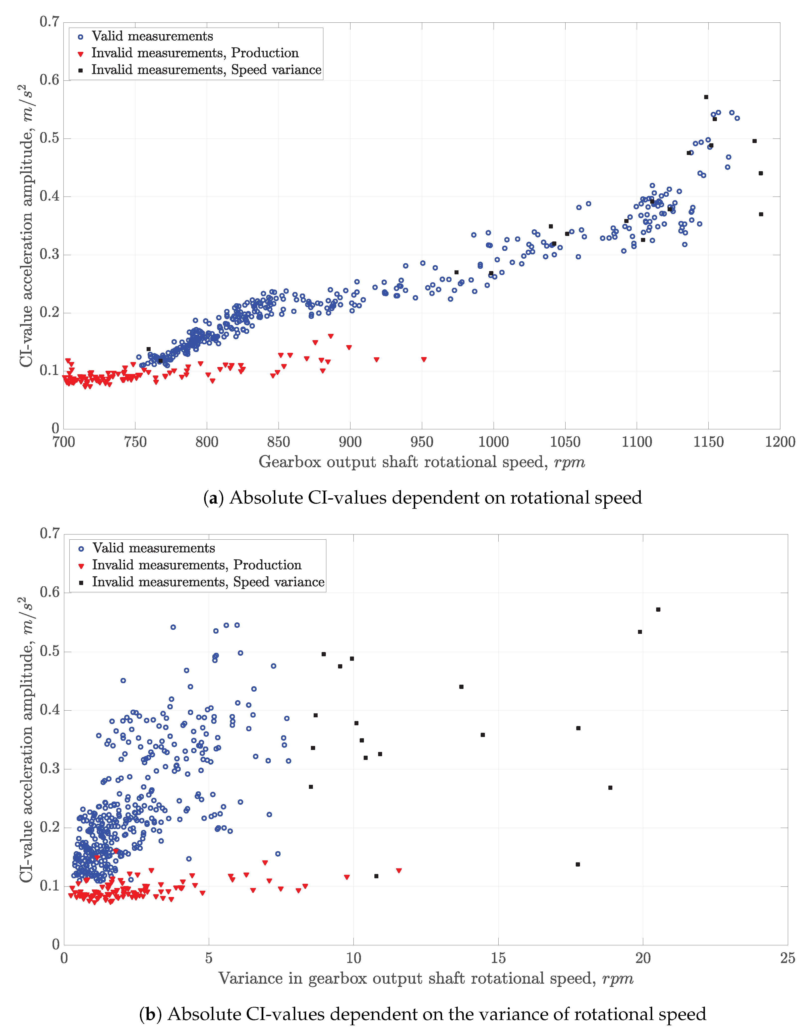
• The variance in rotational speed of the gearbox output shaft during the measurement time of the vibration measurements was shown to detrimentally influence the results, with singular peaks appearing in the trended normalized difference value between the prediction and the CI-results. This increase in non-stationarity lowered the noise level of the spectrum and the predictions were thereby overestimated, causing peaks in the normalized difference interfering. Thereby, the elimination of CI-values where the rotational speed variance was deemed too high from the analysis is recommended.
• By implementing the proposed ANN procedure on the planet bearing failure case it was shown to improve the sensitivity to such a degree that the defect could be detected, which was not possible by the CI-values only.

References

1. GWEC. Global Wind Report 2019; Technical report; Global Wind Energy Council: Brussels, Belgium, 2020. [Google Scholar]
2. Crowther, A.; Ramakrishnan, N.; Zaidi, N.A.; Halse, C. Sources of time-varying contact stress and misalignments in wind turbine planetary sets. Wind Energy 2011, 14, 637–651. [Google Scholar] [CrossRef]
3. Sheng, S. Wind Turbine Gearbox Reliability Database, Condition Monitoring, and Operation and Maintenance Research Update; Technical Report No. NREL/PR-5000-68347; National Renewable Energy Lab. (NREL): Golden, CO, USA, 2017. [Google Scholar]
4. Hameed, Z.; Hong, Y.S.; Cho, Y.M.; Ahn, S.H.; Song, C.K. Condition monitoring and fault detection of wind turbines and related algorithms: A review. Renew. Sustain. Energy Rev. 2009, 13, 1–39. [Google Scholar] [CrossRef]
5. Samanta, B.; Al-Balushi, K.R. Artificial neural network based fault diagnostics of rolling element bearings using time-domain features. Mech. Syst. Signal Process. 2003, 17, 317–328. [Google Scholar] [CrossRef]
6. Castejón, C.; Lara, O.; García-Prada, J.C. Automated diagnosis of rolling bearings using MRA and neural networks. Mech. Syst. Signal Process. 2010, 24, 289–299. [Google Scholar] [CrossRef]
7. Unal, M.; Onat, M.; Demetgul, M.; Kucuk, H. Fault diagnosis of rolling bearings using a genetic algorithm optimized neural network. Meas. J. Int. Meas. Confed. 2014, 58, 187–196. [Google Scholar] [CrossRef]
8. de Almeida, L.F.; Bizarria, J.W.P.; Bizarria, F.C.P.; Mathias, M.H. Condition-based monitoring system for rolling element bearing using a generic multi-layer perceptron. J. Vib. Control 2015, 21, 3456–3464. [Google Scholar] [CrossRef] [Green Version]
9. Li, G.; Deng, C.; Wu, J.; Chen, Z.; Xu, X. Rolling bearing fault diagnosis based on wavelet packet transform and convolutional neural network. Appl. Sci. 2020, 10, 770. [Google Scholar] [CrossRef] [Green Version]
10. Zhang, Z.; Wang, Y.; Wang, K. Fault diagnosis and prognosis using wavelet packet decomposition, Fourier transform and artificial neural network. J. Intell. Manuf. 2013, 24, 1213–1227. [Google Scholar] [CrossRef]
11. Widodo, A.; Yang, B.S. Support vector machine in machine condition monitoring and fault diagnosis. Mech. Syst. Signal Process. 2007, 21, 2560–2574. [Google Scholar] [CrossRef]
12. Soualhi, A.; Medjaher, K.; Zerhouni, N. Bearing health monitoring based on hilbert-huang transform, support vector machine, and regression. IEEE Trans. Instrum. Meas. 2015, 64, 52–62. [Google Scholar] [CrossRef] [Green Version]
13. Saari, J.; Strömbergsson, D.; Lundberg, J.; Thomson, A. Detection and identification of windmill bearing faults using a one-class support vector machine (SVM). Meas. J. Int. Meas. Confed. 2019, 137, 287–301. [Google Scholar] [CrossRef]
14. Saravanan, N.; Siddabattuni, V.N.S.K.; Ramachandran, K.I. A comparative study on classification of features by SVM and PSVM extracted using Morlet wavelet for fault diagnosis of spur bevel gear box. Expert Syst. Appl. 2008, 35, 1351–1366. [Google Scholar] [CrossRef]
15. Cabrera, D.; Sancho, F.; Sánchez, R.V.; Zurita, G.; Cerrada, M.; Li, C.; Vásquez, R.E. Fault diagnosis of spur gearbox based on random forest and wavelet packet decomposition. Front. Mech. Eng. 2015, 10, 277–286. [Google Scholar] [CrossRef]
16. Wang, Z.; Zhang, Q.; Xiong, J.; Xiao, M.; Sun, G.; He, J. Fault Diagnosis of a Rolling Bearing Using Wavelet Packet Denoising and Random Forests. IEEE Sens. J. 2017, 17, 5581–5588. [Google Scholar] [CrossRef]
17. El-Thalji, I.; Jantunen, E. A summary of fault modelling and predictive health monitoring of rolling element bearings. Mech. Syst. Signal Process. 2015, 60–61, 252–272. [Google Scholar] [CrossRef]
18. de Azevedo, H.D.M.; Araújo, A.M.; Bouchonneau, N. A review of wind turbine bearing condition monitoring: State of the art and challenges. Renew. Sustain. Energy Rev. 2016, 56, 368–379. [Google Scholar] [CrossRef]
19. Liu, Z.; Zhang, L. A review of failure modes, condition monitoring and fault diagnosis methods for large-scale wind turbine bearings. Meas. J. Int. Meas. Confed. 2020, 149, 107002. [Google Scholar] [CrossRef]
20. Tautz-Weinert, J.; Watson, S.J. Using SCADA data for wind turbine condition monitoring—A review. IET Renew. Power Gener. 2017, 11, 382–394. [Google Scholar] [CrossRef] [Green Version]
21. Yang, W.; Court, R.; Jiang, J. Wind turbine condition monitoring by the approach of SCADA data analysis. Renew. Energy 2013, 53, 365–376. [Google Scholar] [CrossRef]
22. Bangalore, P.; Letzgus, S.; Karlsson, D.; Patriksson, M. An artificial neural network-based condition monitoring method for wind turbines, with application to the monitoring of the gearbox. Wind Energy 2017, 20, 1421–1438. [Google Scholar] [CrossRef]
23. Singh, J.; Azamfar, M.; Li, F.; Lee, J. A systematic review of machine learning algorithms for PHM of rolling element bearings: Fundamentals, concepts, and applications. Meas. Sci. Technol. 2020, 32, 012001. [Google Scholar] [CrossRef]
24. Rumelhart, D.E.; Hinton, G.E.; Williams, R.J. Learning Internal Representations by Error Propagation; Technical report; California Univ. San Diego La Jolla Inst. for Cognitive Science: La Jolla, CA, USA, 1985. [Google Scholar]
25. McFadden, P.D.; Smith, J.D. Vibration monitoring of rolling element bearings by the high-frequency resonance technique—A review. Tribol. Int. 1984, 17, 3–10. [Google Scholar] [CrossRef]
26. Harris, T.A.; Kotzalas, M.N. Essential Concepts in Bearing Technology, 5th ed.; CRC Press: Boca Raton, FL, USA, 2006. [Google Scholar]
27. Strömbergsson, D.; Marklund, P.; Berglund, K.; Larsson, P.E. Bearing monitoring in the wind turbine drivetrain: A comparative study of the FFT and wavelet transforms. Wind Energy 2020, 23, 1381–1393. [Google Scholar] [CrossRef] [Green Version]
Figure 1. Schematic of an artificial neural network.
Applsci 11 03588 g001
Figure 2. Normalized CI-values from FFT spectra in blue and WPT in black on enveloped measurements from failure case 1 in (a) and failure case 2 in (b).
Applsci 11 03588 g002aApplsci 11 03588 g002b
Figure 3. Normalized condition indicator CI-values from FFT spectra on 0–5 kHz and 0–10 kHz frequency range enveloped measurements in blue and red respectively from failure case 3.
Applsci 11 03588 g003
Figure 4. Absolute CI-values dependent on rotational speed in (a) and variance in rotational speed in (b). CI-values filtered out with respect to the generator not producing in red and CI-values filtered out with respect to high variance in rotational speed in black.
Applsci 11 03588 g004
Figure 5. Gearbox output shaft bearing failure case 1, enveloped FFT CI-values. Comparison of ANN’s predicted CI-values in red and true CI-values in blue at the top graph in (a) and normalized difference between them at the bottom graph without rotational speed variance data filtration. Normalized difference between predicted and true CI-values with rotational speed variance data filtration in (b).
Applsci 11 03588 g005
Figure 6. Gearbox output shaft bearing failure case 1, enveloped WPT CI-values. Comparison of ANN’s predicted CI-values in red and true CI-values in blue at the top graph in (a) and normalized difference between them at the bottom graph without rotational speed variance data filtration. Normalized difference between predicted and true CI-values with rotational speed variance data filtration in (b).
Applsci 11 03588 g006
Figure 7. Planet bearing failure case 2, enveloped FFT CI-values. Comparison of ANN’s predicted CI-values in red and true CI-values in blue at the top graph and normalized difference between them at the bottom graph.
Applsci 11 03588 g007
Figure 8. Failure case 2, planet bearing failure, enveloped WPT CI-values. Comparison of ANN’s predicted CI-values in red and true CI-values in blue at the top graph and normalized difference between them at the bottom graph.
Applsci 11 03588 g008
Figure 9. Gearbox output shaft bearing failure case 3, CI-values trended per day of the dataset starting at 0 from FFT spectra on enveloped measurements with a 0–5 kHz frequency range. Comparison of ANN’s predicted CI-values in red and true CI-values in blue at the top graph and normalized difference between them at the bottom graph.
Applsci 11 03588 g009
Figure 10. Gearbox output shaft bearing failure case 3, enveloped FFT CI-values from measurements with a 0–10 kHz frequency range trended per day of the dataset starting at 0. Comparison of ANN’s predicted CI-values in red and true CI-values in blue at the top graph and normalized difference between them at the bottom graph.
Applsci 11 03588 g010