Abstract
Sheet piles are significantly more prone to advanced corrosion rates due to accelerated low water corrosion. Current inspection and assessment techniques are costly, time-consuming and labour-intensive. Guided wave testing (GWT) has gained increased attention due to its capability of screening long distances; however, it has not been used previously to inspect the active zone in steel sheet piles. This paper focuses on the numerical modelling of wave propagation and defect detection in U-shaped piles to demonstrate the capabilities of GWT for the inspection of non-accessible areas of steel sheet piles. Two shear transducer arrays were designed, bearing high mode purity and directionality. A wave propagation comparison study concluded that the back wall reflection signal from the web of a U-pile was 11.5% higher than the respective signal from the plate, and the excitation signal in the flange, at 5.65 m and 7.12 m, was respectively 35% and 46% less than the excitation signal in the web at the same distance. Defect reflection, measured from five representative defect scenarios, ranged from 7.5 to 47% of the signal amplitude in the web of the pile and 5 to 32.5% in the flange of the pile.
1. Introduction
Structural steel is the most widely used material of choice for the structures used in coastal and offshore locations. It offers many benefits, including durability and simplicity of fabrication, and facilitates relatively cost-effective solutions [1,2]. Although structural steel offers many advantages, corrosion is a major problem for many industries, including the marine and offshore industry [3,4]. It is the main cause of deterioration for waterfront steel structures. There are five other causes that deteriorate structural steel in the offshore industry: overloading, fatigue, abrasion, material loss and weakening of structural connections [5]. Recently it has been acknowledged that sheet piles made of structural steel are significantly more prone to advanced corrosion rates due to accelerated low water corrosion (ALWC) [2]. ALWC rapidly compromises the integrity of affected structures with major implications for safe operation and leads to significant costs for repair or replacement. ALWC is a type of microbiologically induced corrosion (MIC) that arises due to the presence of sulphates in marine environments. Sulphate reducing bacteria (SRB) convert sulphates into hydrogen sulphide (H2S), causing anaerobic corrosion. The H2S is converted by sulphide oxidising bacteria (SOB) into sulphuric acid (H2SO4). This electrolysis process never reaches the state of equilibrium due to the oxidation of hydrogen formed on the steel surface. The non-equilibrium state caused by this biochemical process accelerates corrosion [6].
The corrosion rates on steel pile surfaces vary non-linearly with increasing depth [2]. In order to reliably access sheet piles, determining the location of the most extreme values of thickness loss is of utmost importance [7]. Therefore, many researchers have adapted sheet pile terminology as shown in Figure 1 [2,6,8]. Marine structure designers have considered corrosion conditions at five different vertical exposure zones in relation to environmental conditions. These exposure zones are defined below:
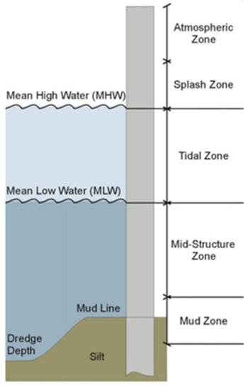
Figure 1.
“Corrosion conditions at five different vertical exposure zones”, adapted from [2].
- Atmospheric zone: The atmospheric zone is located between the top of the pile and the splash zone as illustrated in Figure 1. In this zone, corrosion can take place at the encapsulation point where the pile is covered with concrete.
- Splash zone: This exposure zone is most vulnerable to corrosion. Observations and findings to date suggest that the greatest corrosion rates and highest thickness loss of steel occurs at the splash zones. This is due to ALWC as explained earlier.
- Tidal zone: This exposure zone is found between the mean high water (MHW) and mean low water (MLW) tides. The tidal zone is alternately submerged and emerged, and therefore the corrosion rate is relatively slow due to partial atmospheric corrosion. This zone may also be prone to concentrated corrosion on fixings such as ladder brackets due to the presence of dissimilar metals.
- Mid-structure zone: This exposure zone is located just below the MLW. Corrosion is particularly active in this zone due to the differential aeration that is established with the upper structure. The highly oxygenated metal top, in the tidal zone, acts as a cathode, whereas the constantly submerged metal below acts as an anode, leading to corrosion.
- Mud zone: The mud zone corresponds to the area just below the mid-structure zone where the pile is buried. Observations and findings to date suggest that this area usually requires very little maintenance. In this exposure zone, corrosion can advance in anaerobic conditions where the soils are either acidic or contain SRB, but such conditions rarely arise.
This paper focuses on the corrosion defects in the tidal zone and mid-structure zone as discussed in Section 3.3. Currently, there are a variety of inspection and assessment techniques available to measure or monitor the deterioration of steel piles and obtain information on the mechanism of onset of corrosion. Initial or periodic monitoring can be carried out using rope access to check the condition of the steel sheet pile [9]. Inspection techniques are usually limited to accessible areas that enable visual and tactile inspection, with some thickness measurements done using ultrasonic testing (UT) equipment. These inspection methods are not only costly but time-consuming and labour-intensive. Alternative testing methods, such as integrity testing and crosshole sonic logging, have been used on cylindrical concrete piles [10]. However, they are not directly relevant to the technique used in this study.
This paper reports an investigation carried out using an advanced non-destructive testing (NDT) technique that uses ultrasonic guided wave (UGW) signals to inspect the full length of steel sheet piles. This technique is known as guided wave testing (GWT) [11]. Substantial effort has been expended on the development of such inspection systems due to their ability to screen long distances from a single source to assess a structure’s integrity. This method is extensively used for the inspection of pipelines in the oil and gas industry, as it can identify defects such as corrosion and erosion up to 50 m in each direction from a single location [12].
GWT has been used previously to inspect steel sheet piles in the dead zone, and this is the first time an attempt has been made to inspect the active zone [13]. The major difficulty is that the waveguide has a complicated transverse profile that is significantly different to those of pipes and rails, where the cross-sectional area is finite and small. The waves are bounded by the upper and lower surfaces of the sheet pile in the thickness direction. However, waves could be reflected from edges in the transverse direction as well as from potential defects that are intended to be detected. Nonetheless, it is possible to arrange phase delays between transducers to focus on sound energy in particular areas in order to avoid reflections from edges on the sheet piles.
This paper is organized as follows. The theoretical background of UGWs is presented in Section 2. The FEA theory and methodology implemented for numerical modelling is reported in Section 3, while numerical modelling and results are discussed in Section 4. Conclusions and future suggested work follow in Section 5.
2. Theoretical Background
2.1. Fundamentals of Guided Waves
Owing to advances being made in the fields of mathematics and mechanics of wave propagation, GWT has become a mainstream NDT inspection technique in the industry [11]. In order to develop a reliable inspection technique using UGW, it is imperative to understand the elastic wave propagation within the structural boundaries. The Navier–Stokes equation of motion for an isotropic elastic unbounded medium is as follows:
where and are Lamé constants, is the displacement vector, is the Laplace operator and is the material density. To simplify, Helmholtz decomposition can be utilised to express in the form of a gradient of a scalar and the curl of the zero divergence vector as shown in Equation (2):
where and are scalar and vector potentials of Helmholtz decomposition, respectively. Then, Equation (1) can be decomposed as two simplified wave equations by substituting Equations (2) and (3) of vector potentials:
where and are the longitudinal and shear wave velocities, respectively.
Based on this derivation, longitudinal waves and shear waves are the two elastic wave types that can travel within solids in any direction. However, solid media with multiple boundaries support several types of wave mode, acknowledged as guided waves [14]. Lamb waves are forms of guided waves that exist in a plate and are guided between two parallel tractions, the upper and lower surface of a plate. Lamb waves can be classified into two types, symmetric and asymmetric modes. Symmetric modes are characterised by particle motion being symmetric with respect to the mid-plane of the plate, whereas asymmetric modes are characterised by particle motion being opposite on either side of the mid-plane [15]. Both of these modes are equally used for structural health monitoring (SHM) and are dispersive in nature. Depending on the specimen geometry and material properties, the number of wave modes increases with pulse excitation frequency [12]. In order to identify these wave modes, guided wave nomenclature was specified as:
where is used to represent the type of vibration mode and denotes the order in which modes arrive. Therefore, the fundamental symmetric and asymmetric modes are referred to as and respectively. Shear modes are also addressed similarly, and the fundamental shear horizontal mode is referred to as . The particle vibration of shear modes is polarized parallel to the surface of the plate. Like Lamb modes, shear modes are dispersive in nature, with the exception of the mode [15]. Therefore, has been the preferred mode of excitation in this study.
Dispersion curves plot the variation of frequency with UGW modes’ velocities, and therefore these curves allow one to evaluate the modes that can be excited at a given frequency [16,17]. The dispersion curves for the S355 steel grade U-pile are shown in Figure 2. The dimensions and material properties of the S355 steel U-pile are listed in Table 1. Figure 3 and Figure 4 illustrate the group velocity and phase velocity dispersion curves, respectively. The dispersion curves were calculated using a graphical user interface for guided ultrasonic waves (GUIGUW), a MATLAB based software that calculates wave propagation characteristics using the SAFE (semi-analytical finite element) technique. GUIGUW allows the user to easily compute any waveguide cross-section with good numerical stability and high computational efficiency [17,18,19].
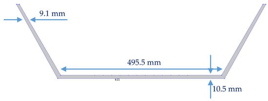
Figure 2.
U-pile dimensions used for generating the dispersion curves and numerical models.

Table 1.
Material properties used to generate the dispersion curves using GUIGUW.
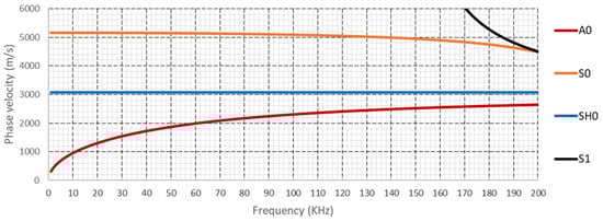
Figure 3.
Phase velocity dispersion curves for U-pile.
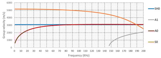
Figure 4.
Group velocity dispersion curves for U-pile.
2.2. Guided Wave Based Defect Detection in Complex Structures
UGWs have been used to inspect plate and pipe structures for decades. These structures have a well-defined yet simple and uniform cross-section, and the principles for generating pure wave modes are well established [20,21]. Pipes are used to transport fluids, and their hollow cylindrical geometry allows UGWs to form an efficient waveguide for longitudinal, flexural and torsional wave modes [22,23].
UGWs have also been applied to pipes with non-accessible areas, such as buried and coated pipes. Kwun et al. investigated the attenuation of T(0,1) mode in a coal-tar-enamel-coated pipe over a frequency range of 5 to 30 kHz and up to a soil cover of 1.7 m depth [24]. Leinov et al. experimentally studied the guided wave propagation and attenuation in an 8 inch schedule-40 carbon steel pipe buried in the sand over a frequency range of 11 to 34 kHz [25]. Hideo N. et al. investigated the attenuation of T(0,1) mode in petrolatum-anticorrosion-grease-coated steel pipe over a 20 to 40 °C temperature range [26].
Guided waves have also been employed for other complex structures, such as rails, wire rope, composite structures and commercial shipping containers. These structures have irregular cross-sectional areas of their profiles. There are many challenges faced in implementing guided waves for complex structures, such as poor signal-to-noise ratio (SNR), high attenuation, poor defect sensitivity and defect localization. Many researchers have proposed signal processing techniques to overcome these challenges. Kazys et al. demonstrated the use of UGW torsional mode in the non-dispersive region to detect defects in a section of rail [13]. Rizzo et al. demonstrated a rail inspection prototype based on UGWs and non-contact probing combined with a distinct signal processing algorithm [27]. Tse et al. applied UGWs on steel wire ropes made of a polymer core and encapsulated by twisted wires [28]. Application of band-pass filtering and discrete wavelet transform on the received signals significantly improved the defect sensitivity and SNR. Pedram et al. illustrated the use of the split-spectrum signal processing technique to improve the defect sensitivity and spatial resolution of UGWs [11]. Results showed a 30 dB improvement in SNR. James S. Hall et al. demonstrated a multipath UGW imaging technique to localise defect detection in two samples: an aluminium plate with three fasteners and sixteen through holes, and a carbon-fibre-reinforced plastic composite panel, each of which had three defects [29]. Clarke et al. evaluated the defect detection ability of a UGW-based SHM system on the door of a commercial shipping container prior to implementing a strategy that involved gating of signals and combining multiple images to significantly improve the defect localisation capability [30,31].
3. FEA Theory and Methodology
The present authors used the COMSOL Multiphysics package to build numerical models for wave propagation and defect detection. Such numerical models helped researchers to carry out their investigations without conducting time-consuming and expensive experiments.
3.1. Design of FEA Model
The model followed the geometry of a U-pile as illustrated in Table 1 and Figure 2. Two transducer arrays, for excitation and receiving of signal data in pulse–echo configuration, were modelled as point sources as shown in Figure 5. The design of modelled transducer arrays is explained in the Array Topology subsection.
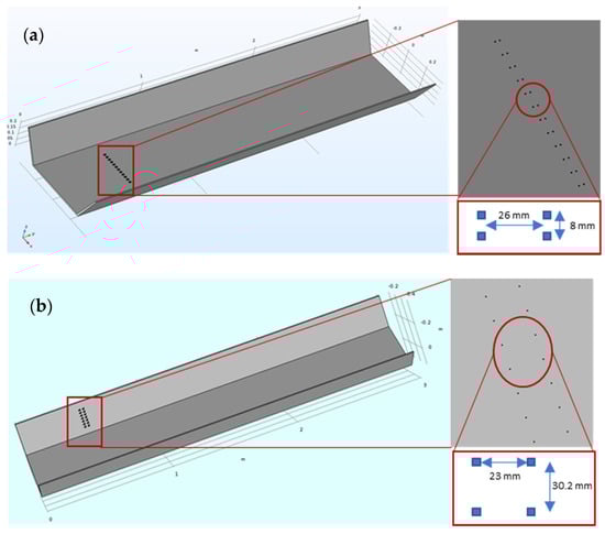
Figure 5.
(a) 12 × 2 configuration shear transducer array for the web of the pile and (b) 7 × 2 configuration shear transducer array for the flange of the pile.
Excitation points were positioned 1 m from one end of the pile. In order to transmit the shear horizontal mode, the point load was applied in the direction along the width of the pile. At each point was applied a 10-cycle sine wave modulated using the Hann window function in Equation (7) below:
where is the excitation central frequency, is time and is the number of cycles.
When setting up a dynamic transient simulation to model wave propagation throughout a structure, it is essential for the mesh to be optimal. In order to avoid potential inaccuracies, it is necessary for meshing and time stepping within the solver to complement each other; as required by the wave equations. Many researchers have recommended using a minimum of 8 mesh elements per wavelength as shown in Equation (8) [17,19,32]:
where is the element size and is the minimum wavelength within in the signal bandwidth. Meshing was kept the same throughout the structure to capture mode conversions and coherent noise generated from reflections.
The duration of the numerical models was decided based on the expected time of arrival () of the signal at the excitation location after reflecting from the simulated defects. The expected was calculated based on the velocity of the mode and the distance travelled by the mode to the end of the pile and back to the excitation location, as shown in Equation (9) below:
where is the total distance travelled and is the velocity of mode at the excitation frequency, obtained from the group velocity dispersion curves generated (Figure 4) for the U-pile.
It is computationally efficient to manually set up the time steps based on the maximum mesh element size. The time steps are chosen to resolve the wave equally over time, whereas meshing resolves the wave equally over the model. Shorter than optimal time steps increase the computation time without significantly improving the results, and longer time steps do not utilise the mesh optimally [33]. The relationship between time step and mesh size is shown in Equation (10):
where CFL is a stability condition. The 0.1 value was selected as it was considered to be near-optimal.
3.2. Trasnsducer Array Arrangement
In elastic waves, the superposition of two or more waves results in interference, which could either be constructive or destructive. The superposition of in-phase waves leads to constructive interference, whereas the superposition of out-of-phase waves leads to destructive interference, as illustrated in Figure 6.
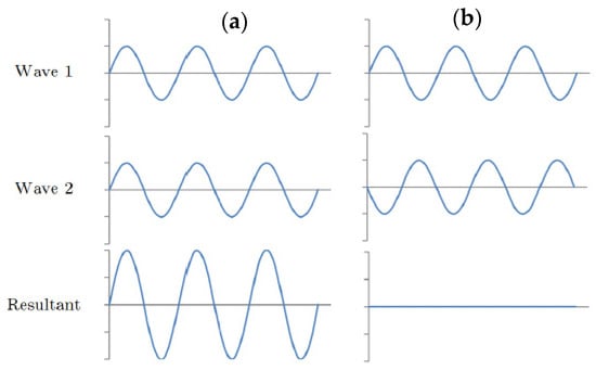
Figure 6.
Superposition of waves showing (a) constructive interference and (b) destructive interference (adapted from [34]).
The transducer array arrangement modelled was determined using the concept of linear superposition analysis (LSA) developed by Hugo Marques [34]. Several researchers have implemented LSA to achieve unidirectional wave excitation with significant mode purity [34,35,36]. The LSA principle is based on the summation of the sound field vectors from each distinct GW source determining the resultant sound field from an array at a given point. The resultant sound field from an array of two UGW sources can be obtained using Equation (11) below:
where
where is a receiver point on a plane, and are the distances between the receiving point and the two corresponding guided wave sources and is the phase velocity.
Using the LSA, Hugo Marques developed a 12 × 2 configuration shear array design that offered sound wave excitation in a single direction with significant mode purity [35]. This dual array design was implemented to achieve desired UGW interference aimed at mode beam directionality control. In order to achieve mode purity and directionality control, appropriate column/row spacing, out-of-phase excitation and time delay were applied. The result was a trade-off between mode destructive interference in one direction with constructive interference in the other, and simultaneous destructive interference of the unwanted Lamb modes in all directions.
In order to optimise the mode purity and directionality, apodisation of the amplitude of excitation signal was applied on transducers across each row. The apodisation function, also known as the tapering function, was achieved by exciting UGW sources across the array with different voltage amplitudes [37]. This resulted in gradually increasing signal amplitude from the outside to the inside of the array, reducing the contribution of outward UGW sources. The rate of apodisation, , was obtained using the following relationship [34]:
where is the number of transducers in the array and is the index number of each transducer.
The 12 × 2 configuration shear transducer array was further improved for the sheet pile inspection by optimising the row and column spacing according to the material properties and web width. Assuming a fixed 8 mm row spacing, the mode directionality and mode purity were evaluated against column spacing ranging from 10 mm to 30 mm, over the frequency range of 20 kHz to 100 kHz. The LSA results obtained for mode directionality and purity, shown in Figure 7, indicated that the 12 × 2 configuration array design with 26 mm column spacing and 8 mm row spacing could excite with relatively high mode purity and directionality at 70 kHz of excitation frequency.
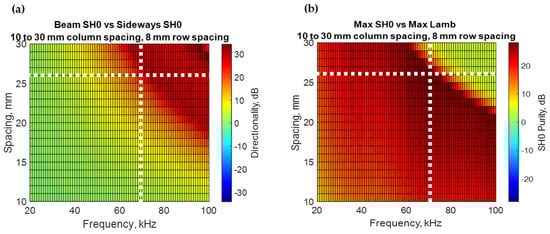
Figure 7.
LSA results for 12 × 2 configuration shear transducer array: (a) directionality and (b) mode purity.
The 12 × 2 configuration shear transducer array was excessively large to inspect the flange of the pile, and therefore a 7 × 2 configuration shear transducer array was also designed for flange inspection. For 30.2 mm row spacing, mode purity and mode directionality was evaluated against column spacing ranging from 10 mm to 30 mm and over the frequency range of 20 kHz to 100 kHz. The LSA results obtained for the 7 × 2 configuration array, shown in Figure 8, indicated that 30.2 mm row spacing and 24 mm column spacing could excite with high mode purity and relative directionality at 70 kHz of excitation frequency.
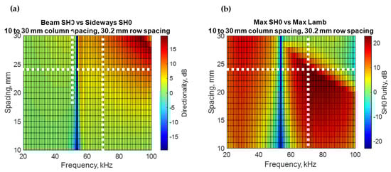
Figure 8.
LSA results for 7 × 2 configuration shear transducer array: (a) directionality and (b) mode purity.
3.3. Simulated Defect Locations
Steel sheet piles are used as foundation to support structures including buildings, towers, bridges and tanks. They are also used at river embankments, cofferdams and bulkheads. The 12 m pile is the commonly installed size in a number of applications and was considered in the current research. Input from experienced field engineers indicated the typical areas of interest where defects exist that can lead to buckling and therefore truly affect the integrity of the pile. Hence, the two defect locations that were selected for numerical modelling were 5.65 m and 7.12 m. Five defect scenarios, listed in Table 2, were considered at the aforementioned defect locations, as illustrated in Figure 9.
Table 2.
Defect scenarios considered.
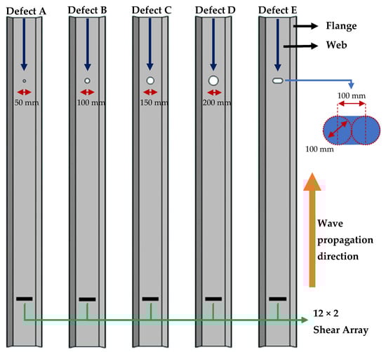
Figure 9.
Defect scenarios using 50 mm, 100 mm, 150 mm, 200 mm diameter defects and a slot defect were considered.
4. Numerical Results and Discussion
Initially, a wave propagation comparison study was conducted between the web and flange of a 7.5 m U-pile and a plate having the same length and cross-sectional area as the web of the pile. This was completed in order to understand the added complexity of the U profile on wave propagation. In the case of wave propagation on the web of the U-pile and the plate, a 12 × 2 configuration shear transducer array, represented by 24 point sources, was placed at 1 m from one end of the web of the pile to excite the 10-cycle signal at 70 kHz central frequency. In the case of wave propagation in the flange of the U-pile, a 7 × 2 configuration shear transducer array, represented by 14 point sources, was placed at 1 m from one end of the flange of the pile to excite the 10-cycle signal at 70 kHz central frequency. Apodisation of the amplitude of excitation signal was applied across each row of transduction points as shown in Figure 10 and Figure 11.
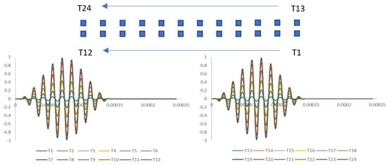
Figure 10.
Apodisation of the amplitude of the excitation signal applied across each row of 12 × 2 array transduction points.
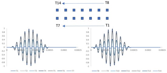
Figure 11.
Apodisation of the amplitude of the excitation signal applied across each row of 7 × 2 array transduction points.
Figure 12a demonstrates how the shear waves propagated on the web of the U-pile. It is evident that as the shear wave propagated, a part of the signal energy travelled into the flanges of the U-pile and interacted with the edges, due to which the signal spread over time. Figure 12b,c illustrates the excitation signal on the web when it reached the distances of 5.65 m and 7.12 m, respectively. It can be noted that the excitation signal at 5.65 m had higher Y and Z displacements due to the higher reflections from the edges at that distance. Figure 13 exhibits the shear wave propagation in the plate travelling in a similar manner as in the web of the U-pile.
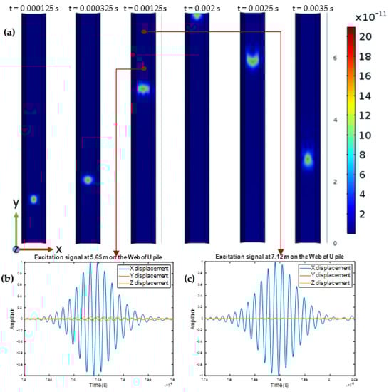
Figure 12.
(a) Shear wave propagation in the web of the U-pile, (b,c) the excitation signal when it reached the distance of 5.65 m and 7.12 m, respectively.
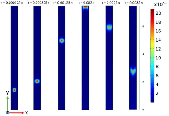
Figure 13.
Shear wave propagation in the plate with the same cross-sectional area as the web of the U-pile.
Figure 14 shows a wave propagation comparison between the plate and the web of the U-pile. Simulated data collection was carried out at 0.5 m ahead of the transduction points in both the plate and the U-pile in order to clearly capture the excitation signal and back wall reflection for comparison purposes. Results were normalized to the excitation signal on the web of the U-pile. The back wall reflection signal from the U-pile web was 11.5% higher than that from the plate. This is because a part of the signal energy reflected from the edges of the plate, leading to destructive interference, whereas in the case of the web of the U-pile, the signal energy travelled through the flanges, avoiding interference.
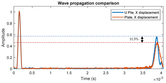
Figure 14.
Wave propagation comparison between the plate and the web of the U-pile.
Figure 15a illustrates how the shear wave propagated in the flange of the U-pile. It can be perceived that as the wave propagated, a part of the signal reflected from the edge of the flange and travelled into the web of the structure, causing the signal to lose energy in the flange. Figure 15b,c illustrates the excitation signal in the flange when it reached the distances of 5.65 m and 7.12 m, respectively. Results were normalized to the excitation signal on the web of the U-pile as shown in Figure 12. The results demonstrate that the excitation signal in the flange at 5.65 m and 7.12 m was respectively 35% and 46% less than the excitation signal in the web at the same distance. This is because, unlike the 12 × 2 configuration, the reduced 7 × 2 configuration forced a reduction in beam directionality and amplitude in favor of a higher mode purity, as shown in Figure 7 and Figure 8.
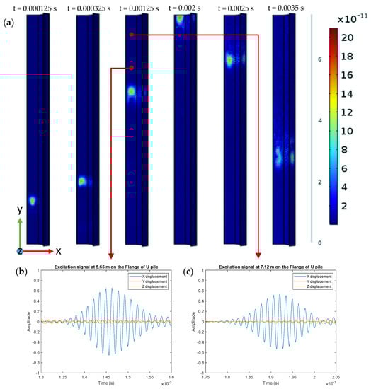
Figure 15.
(a) Shear wave propagation in the flange of the U-pile, (b,c) the excitation signal when it reached the distances of 5.65 m and 7.12 m, respectively.
The numerical models for the following case studies were solely focused on obtaining the reflections from defects. In order to capture pure reflection from defects, a low reflecting boundary condition was applied on the opposite end of the U-pile model. Therefore, U-piles with lengths of 7 m and 7.5 m were modelled instead of 12 m in order to make significant savings in time and computational resources. These case studies were conducted in order to understand the defect detection capability of UGWs on U-shaped steel sheet piles.
4.1. Defect Case Study 1: Defects Placed at 5.65 m for Both Web and Flange
Five defect scenarios listed in Table 2 were modelled on both the web and flange of a 7 m U-pile. Figure 16 and Figure 17 show the superposed results obtained from defects located at 5.65 m on the web and flange, respectively. These results were normalized to the excitation signal as displayed in Figure 16a and Figure 17a. Figure 16b and Figure 17b show defect reflection, i.e., the percentage of excitation signal reflecting from the defect. It was noted that the defect reflection increased with an increase in the size of the defect.
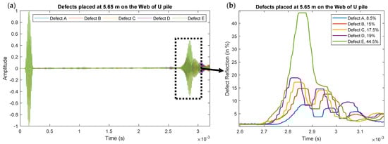
Figure 16.
(a) Results obtained from the defects placed at 5.65 m on the web of the U-pile. (b) Defect reflection results from the respective defects.
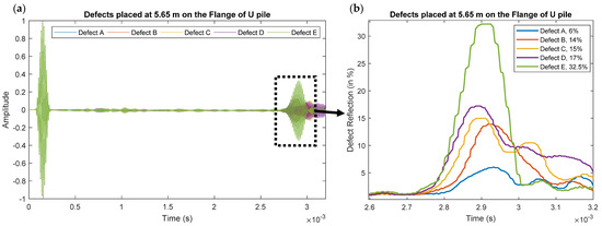
Figure 17.
(a) Results obtained from the defects placed at 5.65 m on the flange of the U-pile. (b) Defect reflection results from the respective defects.
In the case of the defects located on the web, defect reflection from Defect A was 8.5% of excitation signal, which increased to 44.5% of excitation signal for the case of Defect E. A similar trend was observed for defects placed on the flange of the pile at the same location. Defect reflection increased from 6% of excitation signal for the case of Defect A to 32.5% of excitation signal for the case of Defect E. In both the web and flange of the U-pile, Defect E had a much higher defect reflection compared to the rest of the defect scenarios. This is because of the shape of this defect, as a larger portion of the defect was perpendicular to the wave propagation direction.
4.2. Defect Case Study 2: Defects Placed at 7.12 m for Both Web and Flange
As in the last case study, the five defect scenarios listed in Table 2 were modelled on both the web and flange of a 7.5 m U-pile. Figure 18 and Figure 19 show the superposed results obtained from defects located at 7.12 m on the web and flange, respectively. These results were normalized to the excitation signal as displayed in Figure 18a and Figure 19a. Figure 18b and Figure 19b show defect reflection, i.e., the percentage of excitation signal reflecting from the defect.
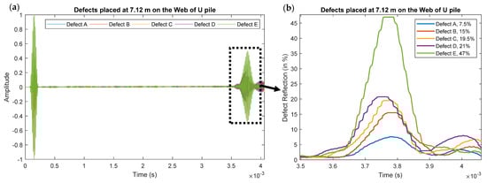
Figure 18.
(a) Results obtained from the defects placed at 7.12 m on the web of the U-pile. (b) Defect reflection results from the respective defects.
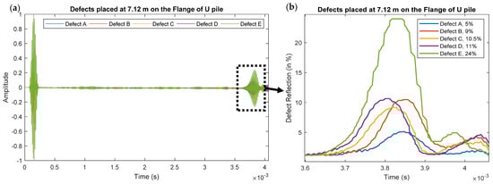
Figure 19.
(a) Results obtained from the defects placed at 7.12 m on the flange of the U-pile. (b) Defect reflection results from the respective defects.
In the case of defects located on the web, defect reflection from Defect A was 7.5% of excitation signal, which increased to 47% of excitation signal for the case of Defect E. A similar trend was observed for defects placed on the flange of the pile at the same location. Defect reflection increased from 5% of excitation signal for the case of Defect A to 24% of excitation signal for the case of Defect E.
The COMSOL models were validated by comparing the theoretical time of arrival () for the expected reflections from the defects at 5.65 m and 7.12 m with the obtained from the numerical models. The theoretical was calculated using the velocity of the mode obtained from the group velocity dispersion curves (Figure 4) for 70 kHz operating frequency. There is approximately 2.5% error in the comparison as presented in Table 3.
Table 3.
Comparison of theoretical and numerical time of arrival.
5. Conclusions and Future Work
In the present study, the authors conducted wave propagation and defect detection modelling using COMSOL to investigate the potential of using GWT as a novel NDT technique for the inspection of steel sheet piles. Due to its non-dispersive nature, the present study preferred for signal excitation. The LSA principle was used to design shear transducer arrays having high mode purity and directionality. A 12 × 2 configuration and a 7 × 2 configuration shear transducer array were modelled for the inspection of the web and flange of a U-shaped steel sheet pile, respectively. Initially, a wave propagation comparison study was conducted between the web of a 7.5 m U-pile and a plate having the same length and cross-sectional area as the web of the pile. Results demonstrated the back wall reflection signal from the web of the U-pile to be 11.5% higher than the reflection signal from the plate. Another wave propagation comparison study was conducted between the web and flange of a 7.5 m U-pile. Results concluded that the excitation signal on the flange at 5.65 m and 7.12 m was respectively 35% and 46% less than the excitation signal on the web at the same distance. To evaluate defect detection capability, models of five defect scenarios, 50 mm hole, 100 mm hole, 150 mm hole, 200 mm hole and 100 mm slot, were considered at two locations, 5.65 m and 7.12 m, on both the web and flange of a U-pile model. Defect detection numerical models were validated by comparing the theoretical and numerical. Defect reflection was measured to demonstrate the ability to use UGW for defect detection in the U-piles.
These numerical models allowed the current authors to carry out their investigations without conducting countless time-consuming and expensive empirical experiments. The next stage for this research is to build only the respective shear transducer arrays modelled for pile inspection and conduct experiments in order to validate the numerical modelling results. Further research will also be completed on transducer characterization to develop novel transducer arrays with higher mode purity and directionality.
Author Contributions
A.D. (Anuj Dhutti) was the lead author and main contributor to this paper. He conducted the numerical investigation and literature review and wrote the original draft of the manuscript. A.D. (Anurag Dhutti) contributed to data analysis and visualization for the manuscript and to reviewing and editing the original manuscript. S.M. contributed by research supervision, project management and coordination of research activity. H.M. created the LSA model and shear transducer array design, and also contributed to reviewing the original manuscript. W.B. contributed to supervision along with the review and editing of the manuscript. T.-H.G. contributed to supervision and project administration along with the review and editing of the manuscript. All authors have read and agreed to the published version of the manuscript.
Funding
This research was funded by Innovate UK, grant number 104362.
Institutional Review Board Statement
Not applicable.
Informed Consent Statement
Not applicable.
Acknowledgments
The authors would like to express gratitude to Innovate UK, Transmission Dynamics Ltd. and TWI Ltd. for all their efforts and contributions to the project and this work.
Conflicts of Interest
The authors declare no conflict of interest.
References
- Hüttenwerke, A.G.D.D. Structural Steel for the Application in Offshore, Wind and Hydro Energy Production: Comparison of Application and Welding Properties of Frequently Used Materials Falko Schröter. Int. J. Microstruct. Mater. Prop. 2011, 6, 4–19. [Google Scholar]
- Sánchez-amaya, J.M. Monitoring the Corrosion of Steel Sheet Piles by Means of Ultrasound and Corrosion Potential Measurements. In Proceedings of the EUROCORR, Freiburg, Germany, 9–13 September 2007; 2007; pp. 9–13. [Google Scholar]
- Popoola, L.T.; Grema, A.S.; Latinwo, G.K.; Gutti, B. Corrosion Problems during Oil and Gas Production and Its Mitigation. Int. J. Ind. Chem. 2013, 4, 1–15. [Google Scholar] [CrossRef]
- Iannuzzi, M.; Barnoush, A.; Johnsen, R. Materials and Corrosion Trends in Offshore and Subsea Oil and Gas Production. NPJ Mater. Degrad. 2017, 1, 2. [Google Scholar] [CrossRef]
- Adler, T.A.; Aylor, D.; Bray, A. Corrosion: Fundamentals, Testing, and Protection; ASM International: Almere, The Netherlands, 2003; Volume 12, p. 459. [Google Scholar]
- Kumar, A.; Stephenson, L.D. Accelerated Low Water Corrosion on Steel Structures in Marine Environments, 27th ed.; Port Technology International: London, UK, 2005. [Google Scholar]
- Schoefs, F.; Yanez-godoy, H. Time-Function Reliability of Harbour Infrastructures from Stochastic Modelling of Corrosion. Eur. J. Environ. Civ. Eng. 2012, 1187–1201. [Google Scholar] [CrossRef]
- Schoefs, F.; Capra, B. Long-Term Stochastic Modeling of Sheet Pile Corrosion in Coastal Environment from On-Site Measurements. J. Mar. Sci. Eng. 2020, 8, 70. [Google Scholar] [CrossRef]
- CONSTRUCTEX Maritime Civil Engineering Services Overview. Available online: https://www.constructex.co.uk/services-overview (accessed on 23 February 2021).
- Niederleithinger, E.; Alexander, T. Concept for Reference Pile Testing Sites for the Development and Improvement of NDT-CE. Available online: https://www.ndt.net/article/ndtce03/papers/v026/v026.htm (accessed on 17 April 2021).
- Pedram, S.K.; Mudge, P.; Gan, T. Enhancement of Ultrasonic Guided Wave Signals Using a Split-Spectrum Processing Method. Appl. Sci. 2018, 8, 1815. [Google Scholar] [CrossRef]
- Catton, P. Long Range Ultrasonic GuidedWaves for the Quantitative Inspection of Pipelines. Ph.D. Thesis, Brunel University London, Uxbridge, UK, 2009. [Google Scholar]
- Kazys, R.; Mudge, P.J.; Sanderson, R.; Ennaceur, C.; Gharaibeh, Y.; Mazeika, L. Development of Ultrasonic Guided Wave Techniques for Examination of Non-Cylindrical Components. Phys. Procedia 2010, 3, 833–838. [Google Scholar] [CrossRef][Green Version]
- Rose, J.L. Waves in Plates. In Ultrasonic Guided Waves in Solid Media; Cambridge University Press: Cambridge, UK, 2014; pp. 76–106. ISBN 9781107273610. [Google Scholar]
- Abbas, M.; Shafiee, M. Structural Health Monitoring (SHM) and Determination of Surface Defects in Large. Sensors 2018, 18, 3958. [Google Scholar] [CrossRef]
- Raisutis, R.; Kazys, R.; Mazeika, L.; Samaitis, V. Propagation of Ultrasonic Guided Waves in Composite Multi-Wire Ropes. Acoust. Waves Adv. Mater. 2016, 9, 451. [Google Scholar] [CrossRef]
- Lowe, P.S.; Lais, H.; Paruchuri, V.; Gan, T.-H. Application of Ultrasonic Guided Waves for Inspection of High Density Polyethylene Pipe Systems. Sensors 2020, 20, 3184. [Google Scholar] [CrossRef] [PubMed]
- Bocchini, P.; Asce, M.; Marzani, A.; Viola, E. Graphical User Interface for Guided Acoustic Waves. J. Comput. Civ. Eng. 2011, 25, 202–210. [Google Scholar] [CrossRef]
- Lais, H.; Lane, K.; Ub, M. Characterization of the Use of Low Frequency Ultrasonic Guided Waves to Detect Fouling. Sensors 2018, 18, 2122. [Google Scholar] [CrossRef]
- Wilcox, P.D.; Lowe, M.J.S.; Cawley, P. Mode and Transducer Selection for Long Range Lamb Wave Inspection. J. Intell. Mater. Syst. Struct. 2001, 12, 553–565. [Google Scholar] [CrossRef]
- Ling, E.H.; Hj, R.; Rahim, A. A Review on Ultrasonic Guided Wave Technology. Aust. J. Mech. Eng. 2020, 4846, 1–13. [Google Scholar] [CrossRef]
- Lowe, M.J.S.; Alleyne, D.N.; Cawley, P. Defect Detection in Pipes Using Guided Waves. Ultrasonics 1998, 36, 147–154. [Google Scholar] [CrossRef]
- Lissenden, J. Applied Sciences Special Issue: Ultrasonic Guided Waves. Appl. Sci. 2019, 18, 3869. [Google Scholar] [CrossRef]
- Kwun, H.; Kim, S.Y.; Choi, M.S.; Walker, S.M. Torsional Guided-Wave Attenuation in Coal-Tar-Enamel-Coated, Buried Piping. Ndt E Int. 2004, 37, 663–665. [Google Scholar] [CrossRef]
- Leinov, E.; Lowe, M.J.S.; Cawley, P. Investigation of Guided Wave Propagation and Attenuation in Pipe Buried in Sand. J. Sound Vib. 2015, 347, 96–114. [Google Scholar] [CrossRef]
- Nishino, H.; Tateishi, K.; Ishikawa, M.; Furukawa, T.; Goka, M. Attenuation Characteristics of the Leaky Mode Guided Wave Propagating in Piping Coated with Anticorrosion Grease. Jpn. J. Appl. Phys. 2018, 57, 07LC02. [Google Scholar] [CrossRef]
- Rizzo, P.; Ni, Y.Q.; Zhu, J.; Hong, T.; Polytechnic, K.; Kong, H. Structural Health Monitoring for Civil Structures: From the Lab to the Field Aerospace Engineering. Adv. Civ. Eng. 2010, 2010, 165132. [Google Scholar] [CrossRef]
- Tse, P.W.; Rostami, J. Advanced Signal Processing Methods Applied to Guided Waves for Wire Rope Defect Detection. In AIP Conference Proceedings; AIP Publishing LLC: College Park, MD, USA, 2016; Volume 1706, p. 030006. [Google Scholar] [CrossRef]
- Hall, J.S.; Michaels, J.E. Multipath Ultrasonic Guided Wave Imaging in Complex Structures. Struct. Health Monit. 2015, 14, 345–358. [Google Scholar] [CrossRef]
- Clarke, T.; Cawley, P.; Wilcox, P.D.; Croxford, A.J. Evaluation of the Damage Detection Capability of a Sparse-Array Guided-Wave SHM System Applied to a Complex Structure Under Varying Thermal Conditions. IEEE Trans. Ultrason. Ferroelectr. Freq. Control 2009, 56, 2666–2678. [Google Scholar] [CrossRef] [PubMed]
- Clarke, T.; Cawley, P. Enhancing the Defect Localization Capability of a Guided Wave SHM System Applied to a Complex Structure. Struct. Health Monit. 2010, 10, 247–259. [Google Scholar] [CrossRef]
- Lais, H.; Lowe, P.S.; Gan, T.; Wrobel, L.C. Ultrasonics-Sonochemistry Numerical Investigation of Design Parameters for Optimization of the in-Situ Ultrasonic Fouling Removal Technique for Pipelines. Ultrason. Sonochem. 2019, 56, 94–104. [Google Scholar] [CrossRef] [PubMed]
- COMSOL Resolving Time-Dependant Waves. Available online: https://www.comsol.com/support/knowledgebase/1118 (accessed on 24 January 2021).
- Marques, H.R. Omnidirectional and Unidirectional SH0 Mode Transducer Arrays for Guided Wave Evaluation of Plate-Like Structures. Ph.D. Thesis, Brunel University London, Uxbridge, UK, 2016. [Google Scholar]
- Niu, X.; Fah, K.; Marques, H.R. Enhancement of Unidirectional Excitation of Guided Torsional T (0, 1) Mode by Linear Superposition of Multiple Rings of Transducers. Appl. Acoust. 2020, 168, 107411. [Google Scholar] [CrossRef]
- Niu, X. Optimising Circumferential Piezoelectric Transducer Arrays of Pipelines through Linear Superposition Analysis Optimising Circumferential Piezoelectric Transducer Arrays of Pipelines through Linear Superposition Analysis. In Proceedings of the Sixth International Symposium on Life-Cycle Civil Engineering (IALCCE 2018), Ghent, Belgium, 28–31 October 2018. [Google Scholar]
- Szabo, T.L. Chapter 6—Beamforming. In Diagnostic Ultrasound Imaging: Inside Out, 2nd ed.; Academic Press: Cambridge, MA, USA, 2014; pp. 167–207. [Google Scholar]
Publisher’s Note: MDPI stays neutral with regard to jurisdictional claims in published maps and institutional affiliations. |
© 2021 by the authors. Licensee MDPI, Basel, Switzerland. This article is an open access article distributed under the terms and conditions of the Creative Commons Attribution (CC BY) license (https://creativecommons.org/licenses/by/4.0/).