1. Introduction
The opportunities within information and communication technology have revolutionized the industry by bringing the fourth industrial revolution, Industry 4.0, into reality. The main enablers of this new era are associated with the opportunities within emerging technologies such as the internet of things, big data, and cloud computing (including detection, diagnosis, and prognosis). These technologies are the fundamentals of Industry 4.0′s core concept, namely the cyber-physical-system that enables converging the physical space of equipment with cyberspace. Therefore, Industry 4.0 is considered as the future scenario of industrial production since it enables a new level of organizing and controlling the entire value chain within the product lifecycle, by creating a dynamic and real-time understanding of cross-company behaviors.
Several case studies [
1] highlight the benefits of digital transformation in the oil and gas (O&G) sector. For example, reducing the upstream operations’ finding and development costs by 5 percent; maintenance costs by 20 percent; overtime cost by 20 percent; downtime by 5 percent (mainly due to predictive maintenance (PdM)); inventory levels for spare parts by 20 percent; while boosting production by a conservative 3 percent in conventional land operations [
1]. However, maintenance management and performance are complex aspects of an asset’s operation that are difficult to justify because of their multiple inherent trade-offs and hidden systems causalities. Nevertheless, companies want to be capable of estimating the lifetime benefits in terms of improving availability and reducing the maintenance management workload, etc., by incorporating intelligent maintenance into the operation and maintenance of their engineering assets to demonstrate (1) how much to invest, (2) when to invest, and (3) the resulting expected lifetime benefits.
Therefore, the industry has really begun to appreciate the benefits of applying modeling and simulation methodologies as a supportive function to enable assessing the behavior and predicting the future outcome of, e.g., maintenance management. For example, Shoreline AS provides a simulation model that helps to simulate possible maintenance alternatives for offshore wind farms and select the most cost-effective by considering operational aspects such as weather forecast, accessibility, and resources i.e., technicians and type of vessel. Moreover, Miriam RAM studio simulates the availability and productivity of O&G installations based on reliability analysis. This helps designers to redesign or design out items to enhance availability and overall equipment effectiveness. These industrial simulation tools shall be enhanced until they capture and are able to estimate all the lifetime benefits of an intelligent maintenance management system. For example, industrial managers are looking forward to estimating the lifetime benefits of PdM and the potential opportunistic maintenance intervals in (1) reducing the corrective maintenance and unintended maintenance events, (2) reducing the preventive maintenance workload and minimizing the planned maintenance campaigns, (3) reducing the level of damage and repair, and (4) extending the lifetime of industrial assets. The desired simulation tool shall support estimating the scheduled maintenance workload (maintenance campaigns), potential corrective maintenance workload, PdM capabilities (effectiveness and earliness), and the planned and potential opportunistic maintenance intervals to perform intelligent maintenance. These basic functions shall enable industrial managers to (1) redesign their maintenance campaigns and potential corrective maintenance (with the help of intelligent maintenance) to fit opportunistic maintenance intervals, (2) reschedule maintenance campaigns at the utilization phase, and (3) redefine their loading and operating profile (optimal profile to produce as high as possible at a deterioration rate as low as possible) either for short-term tactical decisions as toleration to utilize the next potential opportunistic maintenance (avoid unintended maintenance visit) or for long-term strategic decisions to extend their assets’ lifetime. For instance, Arun [
2] illustrates how the change in loading profile (from stand-by redundancy to preschedule redundancy) extends the asset lifetime. In this case study, two out of three crude oil pumps were operating continuously, while one pump was in stand-by mode functioning as redundancy (triggered once one of the other two pumps fail). Following this, the company decided to change the operating policy and run each pump based on time, whereas each pump was operating for two months followed by one month in redundancy (monthly shift between the pumps to ensure that two pumps were running continuously).
The state-of-the-art of simulation models for maintenance practices shows three schools of thinking: discrete event, system dynamics, and agent-based modeling. The discrete-event simulation models for maintenance services and failure events are nicely summarized by Alabdulkarim, Ball et al. [
3]. These models have the objective of independently simulating preventive maintenance and corrective maintenance events (due to probabilistic failures) and consider them as discrete events that return the asset to a state of “as good as new”. First, maintenance practitioners and researchers [
4,
5] have noticed that preventive maintenance has a long-term effect on corrective maintenance and maintenance resources, and they defined the “shift the burden” phenomenon. Second, they noticed that preventive maintenance activities fix the symptoms of failures but might not fix the fundamental problem or cause of the propagating deterioration. Therefore, the system dynamics approach came as the second wave with its ability to model interactions (causalities) between maintenance policies (corrective and preventive) to enable the field of maintenance simulation to study the effect of several and mixed maintenance policies e.g., total productive maintenance [
5], reliability centered maintenance [
6], overall equipment effectiveness [
7], and condition-based maintenance (CBM) [
8,
9,
10,
11]. In this context, simulation models involving maintenance policies using systems dynamics are nicely summarized by Linnéusson, Ng et al. [
12]. In fact, system dynamics models are well known for their high level and abstractive representations (they consider the entire industrial system as one single system), which made maintenance practitioners and researchers search for another approach that models the individual behaviors (where they can decompose the system, but with traceable connections). Therefore, the third wave of maintenance simulation started with agent-based modeling where multi-agent models, multi-simulation models, and individual state-transition (statechart) were enabled. The agent-based models for maintenance simulation are still few, but rapidly growing [
2,
13,
14,
15].
The literature clearly introduces two research gaps. First, none of the existing simulation models have modeled the deterioration based on loading. Second, a model that includes the PdM capabilities of detection, diagnosis, and prediction processes is missing. In summary, to get the lifetime benefits of the referred simulation models and make them fit with the required above-mentioned functionalities (opportunistic maintenance intervals, PdM, and load-based deterioration), further contributions are required. In fact, the future simulation model required shall be able to consider: (1) the individual agent (physical component and failure modes), as Endrerud, Liyanage et al. [
14] have done, besides, (2) modeling the PdM module, as Adegboye, Fung et al. [
15] have done, (3) modeling the asset determination based on loading function as Arun [
2] has done, and (4) modeling opportunistic maintenance intervals and leveraging PdM into these intervals in terms of intelligent maintenance.
Table 1 highlights what is covered by the three latter studies and the missing scientific contribution (research gap) required to enable simulating intelligent maintenance operations.
Therefore, the purpose and scientific contribution of this work is to develop a novel multi-method simulation model that enables estimating the lifetime benefits of an industrial asset, whereas intelligent maintenance is utilized as mixed maintenance strategies and the PdM is leveraged into opportunistic intervals.
Leveraging PdM requires an enhanced level of detection, diagnosis, and prognosis [
16] with an integrated load-based deterioration model. To be more specific, the desired simulation model shall enable simulating the behavior of several maintenance strategies and fulfill specific industrial requirements to ensure its effectiveness, fitness to purpose, and adaptability. The desired model shall enable maintenance engineers to (1) allocate the scheduled maintenance campaigns for each component and differentiate between campaigns that lead to operational unavailability and not, (2) simulate the potential failure events and associated corrective maintenance events, and utilize their real historical failure and maintenance data or data extracted from the well-known failure database, i.e., the offshore and onshore reliability data handbook (OREDA) [
17], or both, (3) assign “failure rate” and “mean time to repair” (MTTR) values for each maintainable item (component level) and associated failure modes, (4) simulate maintenance events that are triggered by CBM or PdM algorithms, (5) assign the capability level of condition monitoring techniques and prediction algorithms [
16], and leverage the predicted failure events into opportunistic maintenance intervals in terms of intelligent maintenance, (6) simulate deterioration process and predict failure events based on realistic (fluctuating, seasonal patterns, stand-by operations, extreme loading intervals) loading and operating profiles. Thus, to build such a model and validate its structure and behavior, a case study of a centrifugal compressor used for natural gas transportation is purposefully selected.
The novel multi-method computational simulation model in this paper is decomposed into four sub-models (1) working state for operational availability and intelligent maintenance, (2) scheduled maintenance states (component level and equipment level) which also presents the opportunistic maintenance intervals, (3) failure states which represent failure modes and triggers for failure events, and (4) corrective maintenance states. Furthermore, to highlight the expected lifetime benefits of intelligent maintenance during 20 years of operation, two main use case scenarios shall be modeled: with and without intelligent maintenance. The latter use case scenario (without intelligent maintenance) has several sub-scenarios that also study the effectiveness of several possible data sources: (1) empiric case study data (experience), (2) manipulated empiric case study data, (3) the OREDA database [
17], and (4) mixed data-input from both the empiric case study and the OREDA database. These four sub-scenarios along with the intelligent maintenance scenario result in a total of five simulated use case scenarios.
The six-step modeling and simulation methodology, presented in the following section, is applied to build the desired novel multi-method computational simulation model that combines agent-based modeling with system dynamics to simulate the five use case scenarios. In this case, the multi-method modeling software Anylogic 8 is utilized.
The rest of this section is organized as follows. First,
Section 2 explains the materials and methodology of this study, which includes the entire six-step simulation modeling methodology adopted.
Section 3 presents the simulated results obtained from the computational model.
Section 4 discusses and validates the findings of this study. Finally,
Section 5 offers some conclusions and makes recommendations for future work.
2. Materials and Methods
In this section, the adopted six-step simulation modeling methodology is presented. Thus, detailed descriptions of how the real-world case study was analyzed, conceptualized, and computerized into a simulation model are presented.
In fact, model-based representations in terms of process modeling and industrial simulation approaches have become a highly embraced tool with their growing complexity and capabilities [
18]. Current literature presents several different methodologies that facilitate the successful development of a simulation model, with the most trusted modeling methodologies being that of [
19,
20,
21], whereas the majority of literature relies on the methodology proposed by Sterman [
21]. Nevertheless, the essence of the different methodologies is quite similar. This research adopts a six-step simulation modeling methodology that extends the essence of Sterman [
21] by allocating additional emphasis on systems analysis and scenario modeling. The adopted six-step modeling and simulation methodology is as follows: (1) System analysis and project planning, (2) Conceptual modeling, (3) Computational modeling, (4) Scenario modeling, (5) Verification and validation, and (6) Visualization. In the following subsections, each step will be described in detail.
2.1. Step 1: System Analysis and Project Planning
The first step in the six-step modeling and simulation process starts with a system analysis addressing the needed fundamentals to attain an understanding of the system’s behavior, i.e., structure, interfaces, processes, interactions, etc. To do so, relevant stakeholders must be addressed, including their needs and requirements to the system under study. Then, the model constraints must be defined by studying, e.g., system context, hierarchy, interface architecture, and functional and physical architecture in greater detail. In addition, other features posing a significance to the purpose must be identified, e.g., politics, market, technology.
The purpose of the system analysis step is to (1) identify the purpose and objective of the simulation, (2) analyze the case study data that is required to conceptualize the maintenance management practices (scheduled, corrective, condition monitoring, opportunistic intervals), especially, workflow, rules, conditions, and actions, (3) analyze the case study data that is required as inputs for the simulation model e.g., failure rates, maintenance service times, and (4) analyze the case study data that is required to validate the simulated behavior e.g., real availability and real corrective maintenance workload.
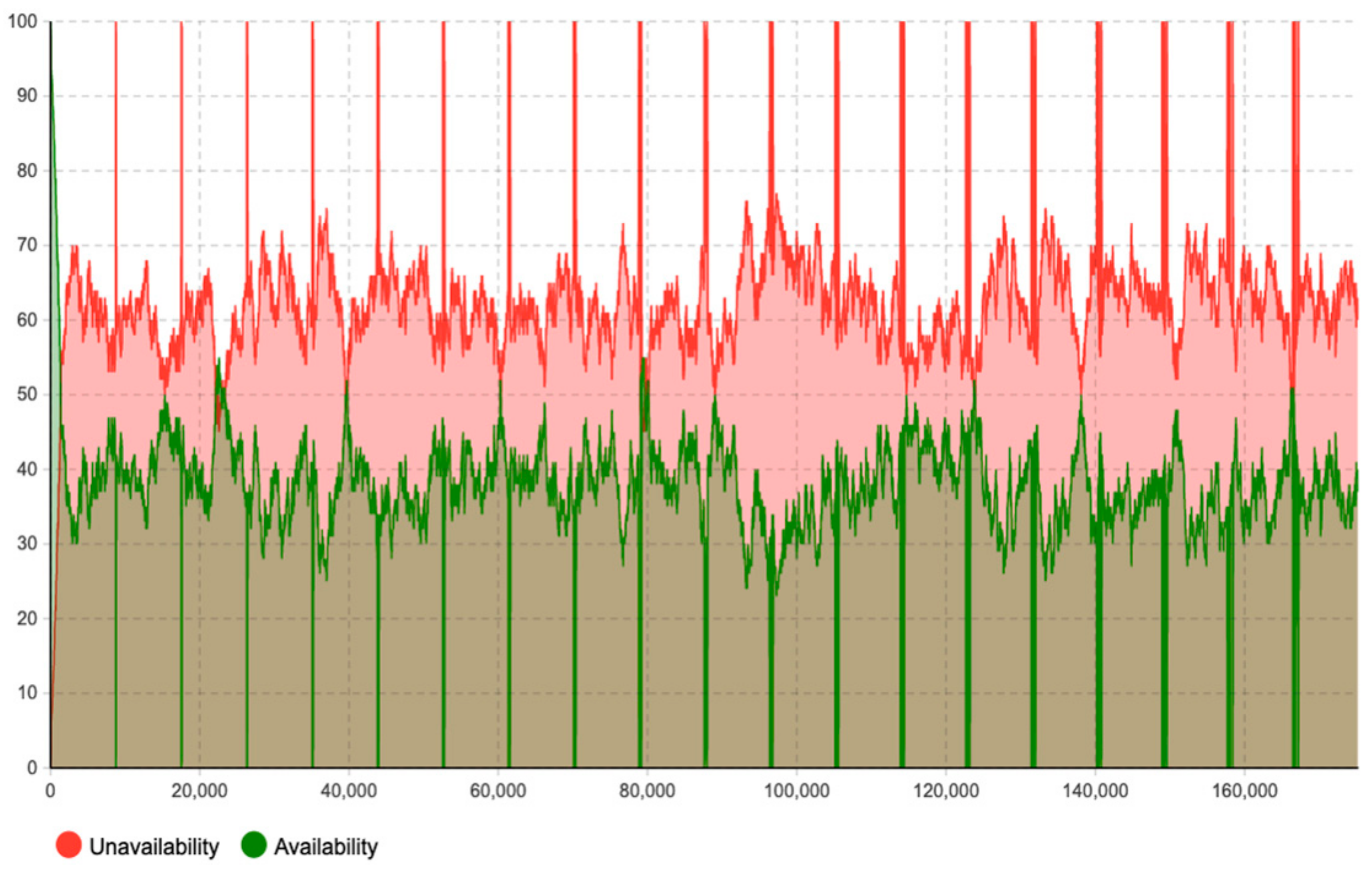
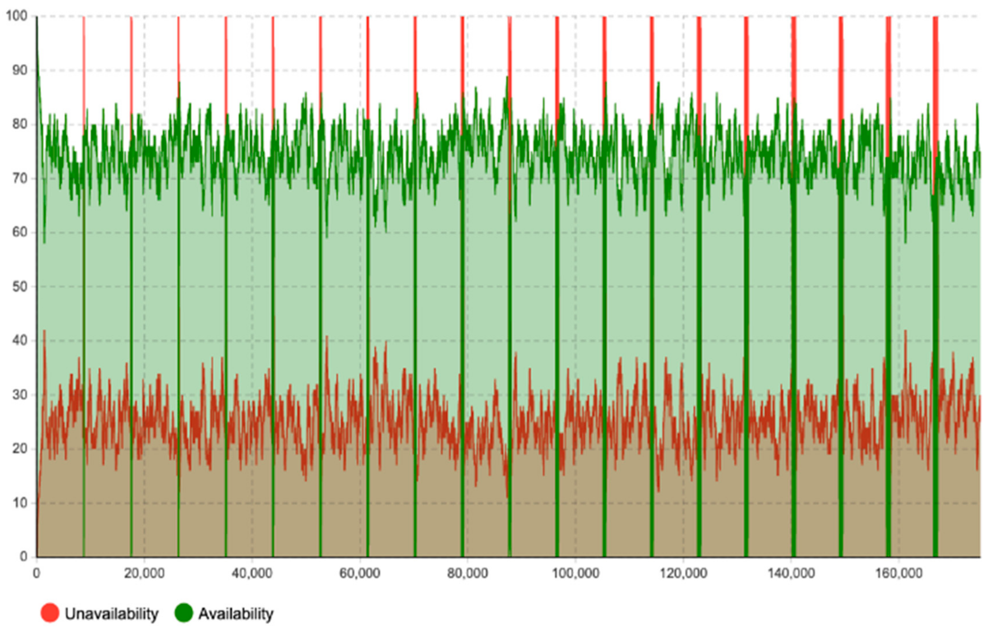
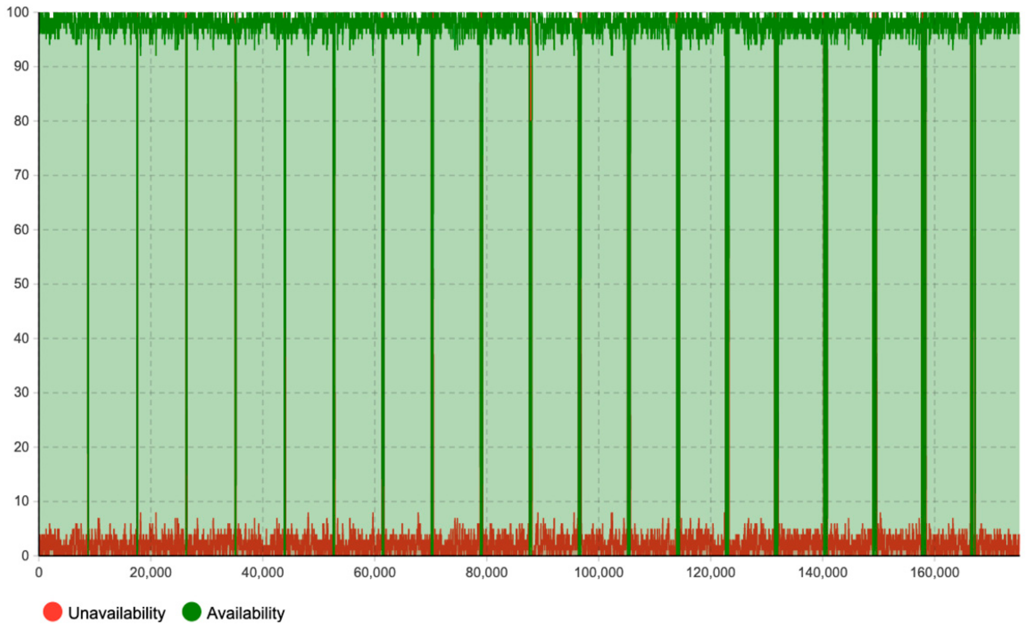
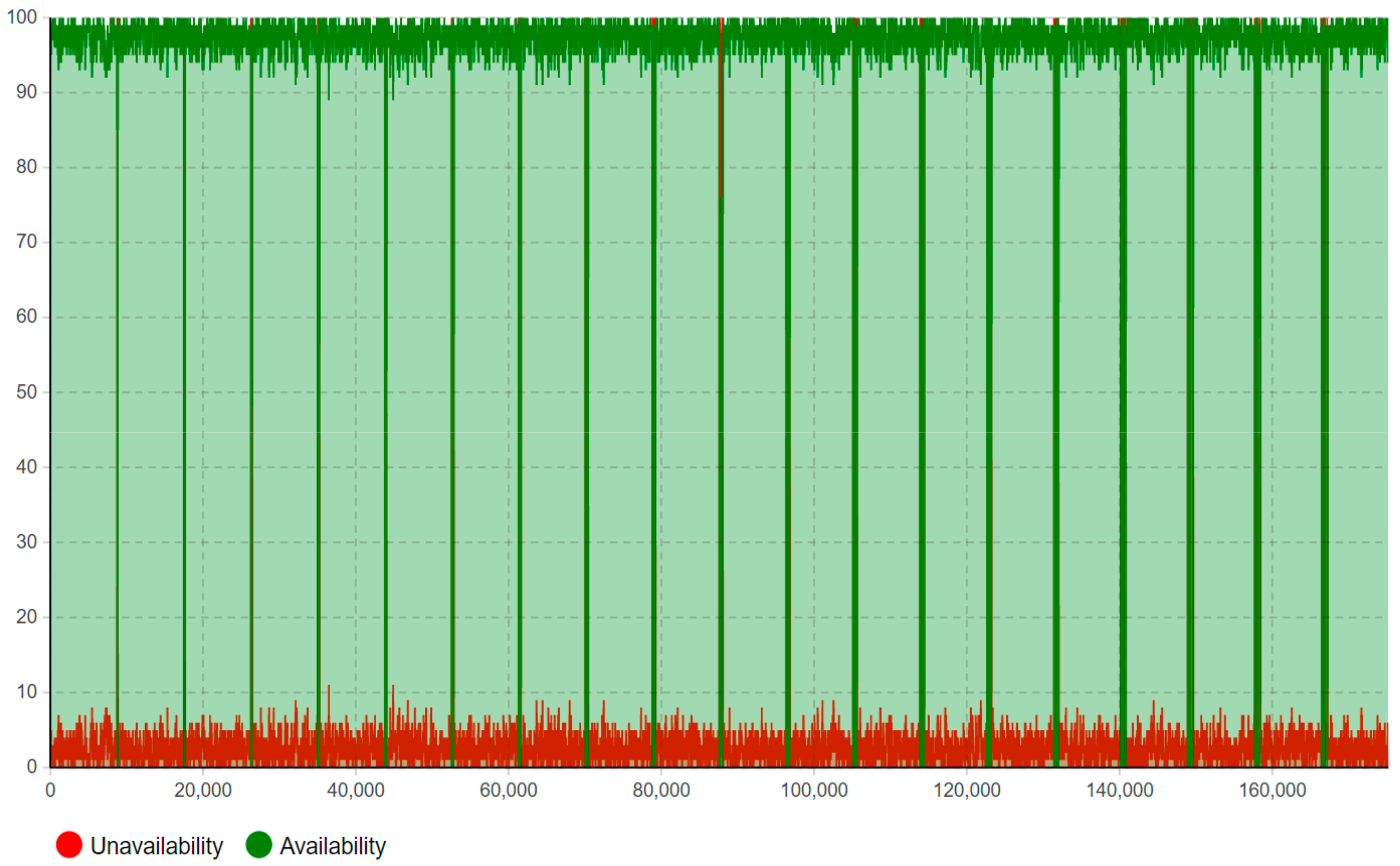
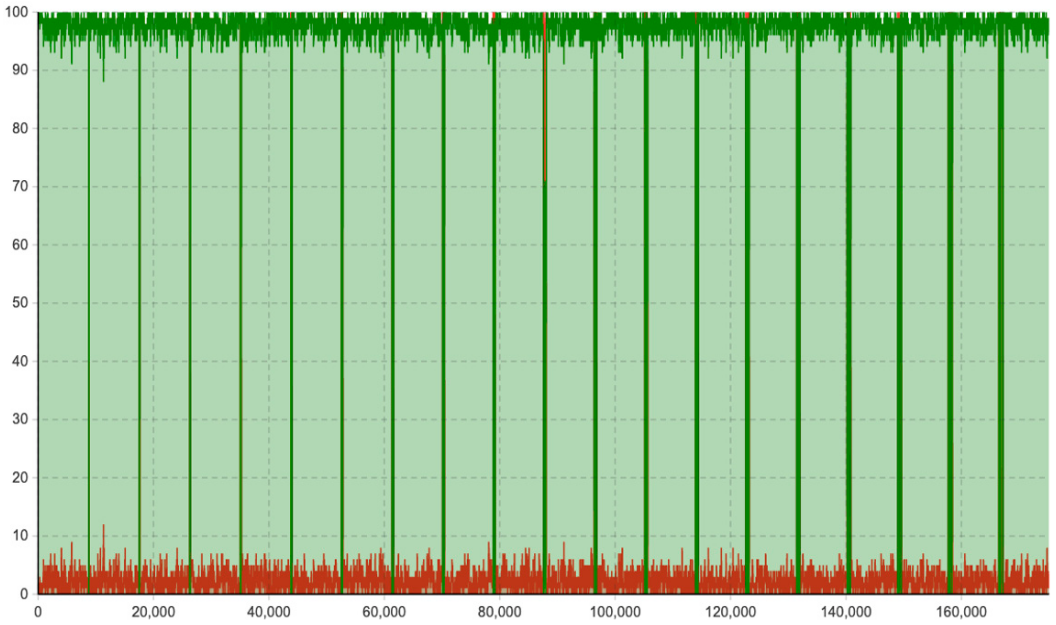
The purpose of the proposed multi-method simulation model is to simulate and estimate the potential lifetime benefits of implementing an intelligent maintenance management system in terms of availability and corrective maintenance workload during a time period of 20 years. Thus, the simulated outputs of the computational model address: (1) operational behavior, (2) maintenance event: timeline and workload, and (3) the occurrence of failures allocated at the component level. It is evident that operational availability is essential for the case company, as the end-user consumption is traceable to industrial operation and human welfare in Europe. Therefore, the operational behaviors including availability and unavailability caused by failures and the need for corrective maintenance are analyzed. This is easiest illustrated through a time-plot diagram showing continuous availability and unavailability as a function of time during operation. The maintenance event timeline of both scheduled maintenance and corrective maintenance is analyzed. First, a scheduled maintenance event timeline is analyzed as it introduces opportunistic maintenance intervals whereas future predicted failures can be allocated. Second, a corrective maintenance event timeline that demonstrates the corrective maintenance events required by the different use case scenarios is analyzed. This is especially interesting when it comes to comparing the corrective use case scenarios with the intelligent maintenance scenario. The maintenance workload is analyzed to demonstrate the allocation of maintenance management. The number of component failures occurring during operation is analyzed to compare different use case scenarios, which supports highlighting the number of corrective maintenance events that can potentially be replaced with intelligent maintenance. In addition, it addresses possible differences in input data originating from the empiric case study and the OREDA database.
To simulate the possible lifetime benefits of incorporating an intelligent maintenance system into the specific case study, data concerning failure rates and MTTR values of the specific case of interest is needed. In addition, data that enables determining the capabilities of detection, diagnosis, and prognosis of such a system is also needed. To do so, an analysis tool that has been developed by the authors on a previous occasion can be adapted [
16]. A more detailed system analysis has already been performed and presented by the authors in [
22].
2.2. Steps 2 and 3: Conceptualization and Computational Modeling
The conceptual modeling is all about synthesizing the developer’s understanding of the real situation analyzed in the “system analysis and project planning” into a conceptual model. This is known as a time-consuming task in comparison to the other steps in the simulation modeling process [
23]. In this context, the authors have already published a paper [
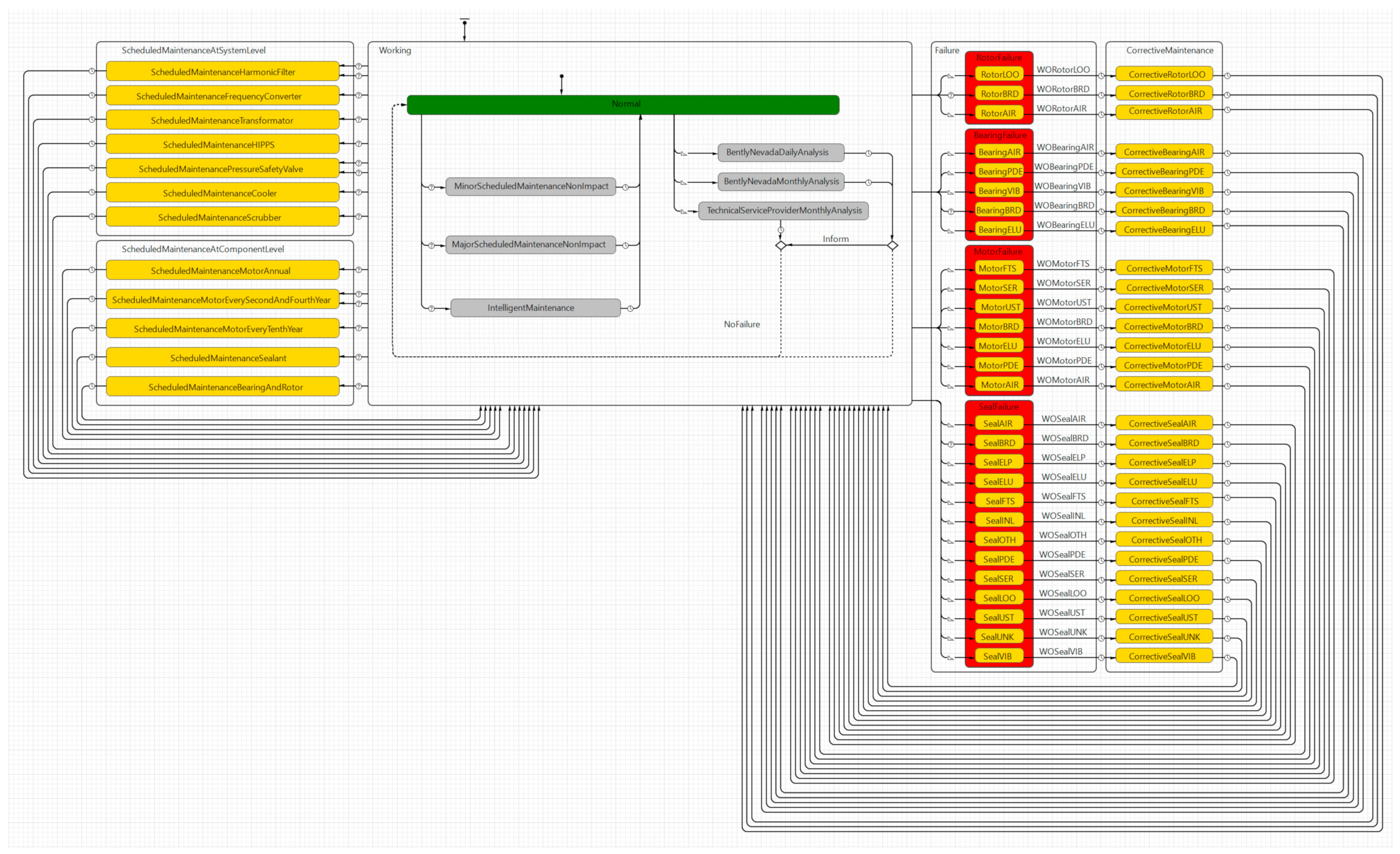
24] where the conceptual model is described using a system dynamic approach. However, the authors later recognized that a multi-method modeling approach combining system dynamics with an agent-based modeling approach, whereas statecharts either triggered by rates, parameters, or conditions connected to system dynamics approaches are used, can enable better modeling of the maintenance policies. The statecharts in
Figure 1 represent the maintenance management process in the case company, specifically for compressor equipment. The statechart is modeled using Anylogic Simulation package (8.5.1) and decomposed into the following four sub-models (1) Working state for operational availability and intelligent maintenance representing the daily operation and maintenance (including condition monitoring) activities that do not affect the operational behavior, (2) scheduled maintenance states (at component level and equipment level), requiring shutdown of the compressor equipment (presents the opportunistic maintenance intervals), (3) failure states, representing failure modes and triggers for failure events, and (4) corrective maintenance states, referring to the corrective maintenance needed to put the compressor equipment back in normal operation post-failure. These four sub-models are illustrated in
Figure 2,
Figure 3 and
Figure 4 and described in more detail in the following subsections, respectively.
2.2.1. Operational Availability and Intelligent Maintenance
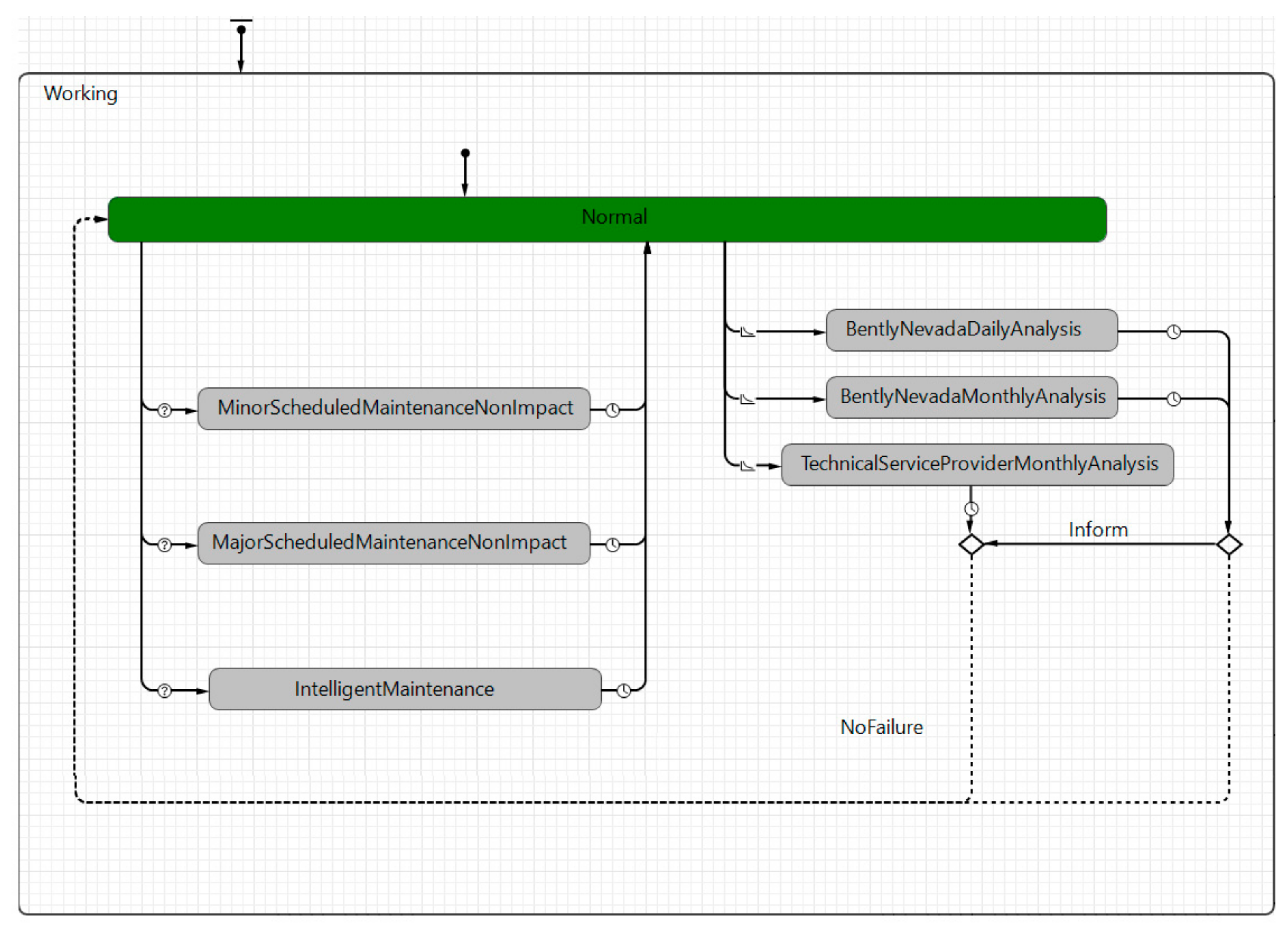
The “working” state is considered as the mother state in
Figure 2, which means that the equipment is available as long as the agent “Compressor” has not triggered a maintenance event requiring equipment stoppage. However, the equipment might be available and running normally in the “normal” state while the condition monitoring system is active, and the equipment health is being checked on a daily and monthly basis (rates). The daily and monthly checks have specific time amounts (i.e., timeout in Anylogic) and might trigger a maintenance event that results in equipment stoppage. The monthly monitoring checks are done by two stakeholders (1) condition monitoring providers and (2) the technical service provider. Moreover, there are minor and major scheduled maintenance work that is taking place while the equipment is running (which does not lead to production stoppage). Furthermore, the PdM might also trigger a maintenance event that can take place in the following opportunistic intervals. This state is named “Intelligent Maintenance” and does not lead to production stoppage as it utilizes potential opportunistic intervals. The time amount for these maintenance events specifically connected to the intelligent maintenance and is extracted based on OREDA data for MTTR.
Table 2 addresses the triggers of the transitions between the different states included in
Figure 2. As seen, the transitions from the “normal” state to the states concerning (minor and major) “scheduled maintenance”, and back again, are triggered by timeouts (specific time interval). The states of “condition monitoring” are triggered by rates. In this case, a conditional transition including a “randomTrue probability distribution” of the input failure data is used to demonstrate the probability of detection. This means that, if the condition is false, the condition monitoring system is not able to detect anything abnormal with the operation and enters the normal working state again. In contrast, if the condition is true, the condition monitoring system has detected abnormal behavior of the system and the presence of failure. The logic of these latter states concerning condition monitoring is not yet incorporated into the computational model, as the extracted failure rates used in this research only contain system failure, and therefore the impact of the monitoring system has already been taking into consideration, indirectly. However, the states are included in the computational model as they pose an impact on the model output in terms of maintenance workload. At last, the “IntelligentMaintenance” is triggered by the flow “OpportunisticMaintenance” from system dynamics and then back to the “normal” state again by a timeout function of 18 h that is extracted from the OREDA database [
17] and traceable to the specific MTTR values of the failure modes monitored in this case study.
2.2.2. Scheduled Maintenance and Opportunistic Maintenance Intervals
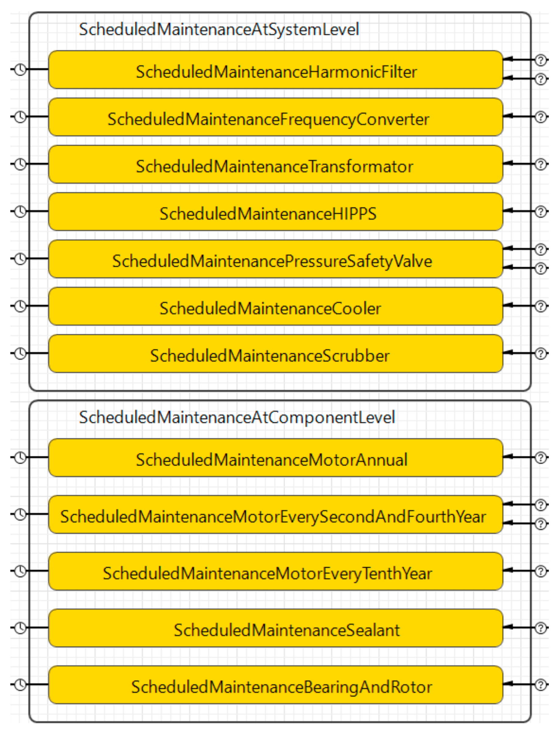
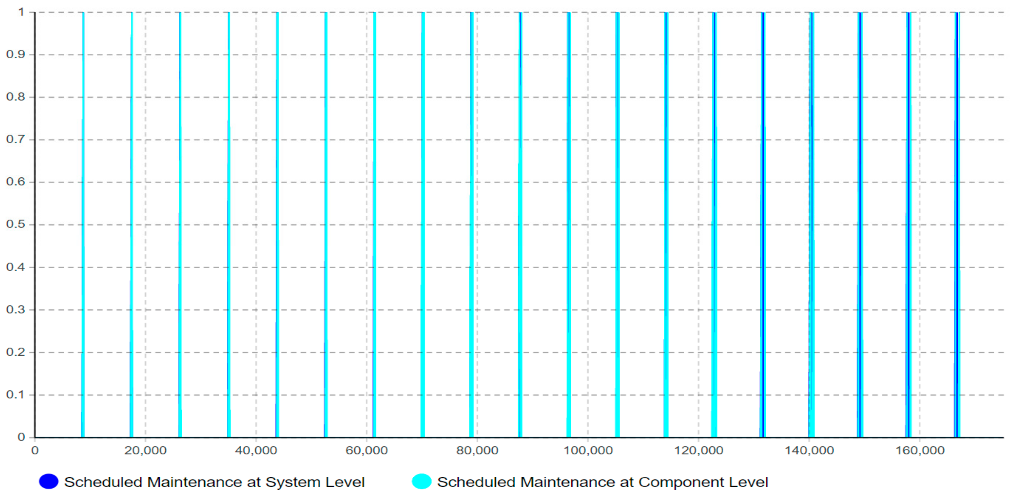
The second sub-model highlights the scheduled maintenance at both system level and component level, as depicted in
Figure 3. More specifically, the scheduled maintenance at both component and system level includes all the scheduled maintenance activities that require stoppage of the system under study. In this case, scheduled maintenance at the component level concerns maintenance activities directly connected to the components of the case study, while scheduled maintenance at the system level focuses on system-level (systems connected to the case study, e.g., scrubber, cooler)—hence, scheduled maintenance causing unavailability of any of these systems requires stoppage of the case study.
Table 3 highlights the triggers that are causing transitions between the different states present in the scheduled maintenance and opportunistic maintenance intervals. In this case, the scheduled maintenance states are triggered by rates that are extracted from the case company data. The durations of the states are, on the other hand, highlighted by triangular distributions either based on the case study data or the OREDA database [
17] (dependent on use case scenario). Since the MTTR values of the scheduled maintenance activities are average values (assuming normal distribution), the triangular distribution is used to incorporate some variance in the data.
The main purpose of modeling the scheduled maintenance at both system and component levels is to address all planned maintenance activities that are causing production stops. These stops are decisive to address as they can be used as opportunistic maintenance intervals in which PdM can be leveraged in terms of intelligent maintenance. Hence, if the intelligent maintenance system enables detecting and predicting the future deterioration propagation of a failure, it can allocate the future required maintenance activity to a coming opportunistic maintenance interval, as long as this interval appears prior to the component fault.
2.2.3. Failure Events and Corrective Maintenance
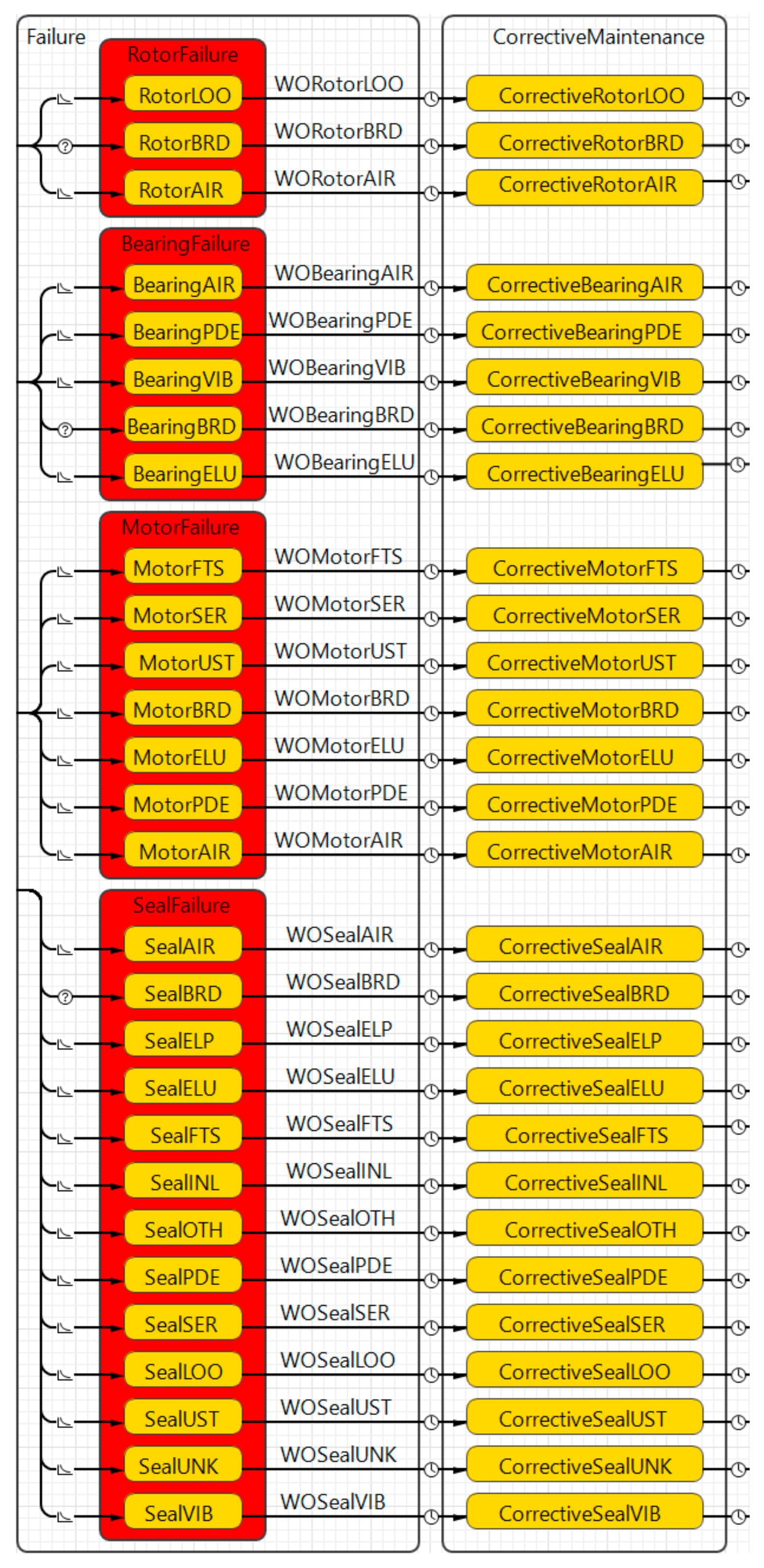
The third sub-model concerns the occurrence of failure events and the associated corrective maintenance actions required to put the component back in operation.
Figure 4 highlights all the failure modes that are associated with the case study based on both the empiric case study data and the OREDA database. The systems analysis step revealed some differences between the failure modes presented in the OREDA database and the ones presented in the case company notification system, as demonstrated in
Table 4. Therefore, only the failure modes represented by the specific scenarios are assigned with values traceable to their specific data source, while the failure modes that do not appear in the specific use case scenario are assigned with a value of zero.
During simulation, the “failures” are triggered by either (1) failure rates that are either extracted from the empiric case study data or the OREDA database [
17] (Scenarios 1–4) or (2) a condition based on deterioration rates supported by Calixto [
25] (only valid for intelligent maintenance and thus Scenario 5). Then, the state of “corrective maintenance” is triggered by timeout functions including a triangular distribution of the MTTR values that are transparent with the specific use case scenario. Since the MTTR values of the corrective maintenance activities are average values (assuming normal distribution), the triangular distribution is used to incorporate some variance in the data. The connection between the states, triggers, values, and data source are summarized in
Table 5.
2.3. Step 4: Scenario Modeling
This section is dedicated to scenario modeling, which facilitates simulating different use case scenarios, and furthermore attaining an understanding of sensitive data and influencing factors identified through the model outputs. To do so, four different use case scenarios are modeled with the purpose of highlighting the associated sensitiveness connected to the model input data i.e., failure rates and MTTR values extracted from either (1) the case study, (2) the well-known OREDA database, [
17] which is highly applied in the O&G industry, or (3) both. In final, the last use case scenario (use case scenario 5) that concerns the loading and deterioration process of the case study is modeled. Its purpose is to highlight the connection between component deterioration, detection, diagnosis, and prognosis purposes in the context of implementing an intelligent maintenance management system into the case study. Therefore, this paper models in total five use case scenarios. The connection between the input data and use case scenarios is summarized in
Table 6 and described in more detail in the following subsections.
2.3.1. Scheduled and Corrective Maintenance Scenarios (1, 2, 3, and 4)
Scenario 1 includes failure rates and associated MTTR values that are extracted from the notification system of the case company. The data is extracted exactly how it is presented in the notification system.
Scenario 2 includes the same data as in the previous scenario. However, the difference in Scenario 2 is that all the values considered as “unreasonably extreme” are replaced with values the authors anticipate to be more reasonable when taking the connection between the specific failure and associated MTTR value into consideration.
Scenario 3 addresses input data involving both failure rates and MTTR values extracted from the OREDA database [
17]. The OREDA database is in fact well-known and highly adopted by O&G companies in connection with analyses concerning risk and technical integrity. In practice, the OREDA database categorizes failure rates in terms of “lower”, “mean”, and “upper” failure rates, and MTTR values in terms of “mean” and “max”. This research adopts the “upper failure rates” and the “max MTTR values”, which experts claim to represent industrial experience the best.
The interesting context of this use case scenario is to highlight whether the case company experiences either higher or lower failure rates and MTTR values in comparison to the OREDA database. This will underpin whether the industry shall be recommended to support integrity assessments based upon their own empiric case study data or the OREDA database, dependent on the associated risk profile (“risk-averse”, “risk-seeking”, etc.).
The estimation of MTTR values originating from the empiric case study data is associated with the highest uncertainty as it depends on two different variables the maintenance personnel need to report (start of maintenance and end of maintenance). Therefore, Scenario 4 replaces the MTTR values from the empiric case study data with the ones presented in the OREDA database.
2.3.2. Intelligent Maintenance Based on Deterioration Modeling (Scenario 5)
One of the main issues of applying failure rates in connection with detection, diagnosis, and prognosis purposes is due to the straight lines in terms of pulses produced by the simulation. In more detail, such straight lines make it difficult, or even impossible, to justify the opportunity to detect, diagnose, and predict future deterioration evolution. The maintenance timeline concept based on failure events is not effective to enable CBM and PdM, as they require deterioration curves instead. Therefore, a deterioration model based on loading that addresses the deterioration curves for the individual component associated with the case study must be modeled.
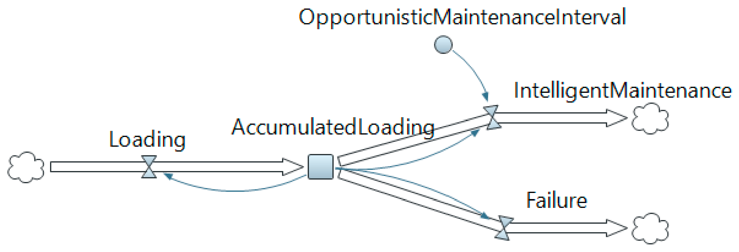
The deterioration modeling process starts by first modeling the component deterioration using system dynamics, depicted in
Figure 5. As seen from the loading model, it contains three different flows: (1) Loading, (2) Failure, and (3) Intelligent maintenance. Furthermore, one stock representing the “accumulated loading”, and one parameter of “Opportunities” which represents the future opportunistic maintenance intervals defined by the scheduled maintenance requiring stops in operation.
The logic of each flow in the deterioration and intelligent maintenance module is described in more detail in
Table 7.
In more detail, the “Loading” flow expresses the entire deterioration process and includes the loading equation of the specific component under study. Such an equation can be established by first identifying a failure distribution that demonstrates the evolution of a specific failure through a deterioration curve. To do so, there exist several failure distributions applied to demonstrate the degradation evolution from a healthy component to a faulty one [
26,
27,
28]. Some of the most applied failure distributions concerning aging equipment are, e.g., “traditional view”, “bathtub curve”, and “slow aging” (linear deterioration) [
29]. However, concerning component deterioration, the distribution of either exponential distribution or power-law distribution is most frequently adopted.
Second, a designed load case that assumes constant loading from the beginning of the operation until it fails must be addressed. Such time to failure can for instance be based on recommendations from the component vendor, estimated through equations offered by the manufacturer (e.g., [
30]) or other reliable data sources (e.g., Calixto [
25] or OREDA [
17]). In final, the suitable deterioration curve identified must be fitted with the time to failure through an iterative simulation process that highlights the entire deterioration process from a healthy component to a faulty one.
In practice, the condition monitoring system monitors the deterioration process of the component during normal operation. If the monitoring system is not capable of detecting and predicting the deterioration, the accumulated deterioration level reaches the designed lifetime (100% deterioration) that triggers the “Failure” flow in system dynamics (
Figure 5), which furthermore triggers the associated “failure” state in the agent-based computational model (shown in
Figure 1). However, if the condition monitoring system is able to detect and predict the level of deterioration propagation prior to component failure, it tries to leverage the PdM event into a coming opportunistic maintenance interval represented by the “OpportunisticMaintenanceInterval” parameter connected to the “IntelligentMaintenance” flow. In this case, the opportunity of leveraging a predicted failure event to a future opportunistic maintenance interval is based on two criteria: (1) when the future opportunistic maintenance intervals appear and (2) the capabilities offered by the specific monitoring system, i.e., levels of detection and prediction that are demonstrated in detail in [
16]. Illustratively, if the condition monitoring system is able to detect component deterioration one week prior to failure and the next opportunistic maintenance interval appears first after four weeks, there exists no opportunity to leverage the PdM into an opportunistic maintenance interval, and corrective maintenance is thus required. In contrast, if the deterioration is detected five weeks prior to component failure and the next opportunistic maintenance interval appears after four weeks, the PdM can be leveraged into the future opportunistic maintenance interval in terms of “intelligent maintenance”. Therefore, exploiting these opportunistic maintenance intervals to perform intelligent maintenance will thus reduce the unplanned operational unavailability and cost (since corrective maintenance is replaced by intelligent maintenance).
At last, this paper presents an illustrative example of how an intelligent maintenance system that enables detecting, diagnosing, and predicting the specific failure mode of breakdown (BRD) of the rotor, bearing, and seal. It is important to emphasize that the transparency between failure modes, and detection, diagnosis, and prognosis processes shall be analyzed individually for the specific condition monitoring system applied. In this context, the authors recommend the future readers perform the analysis presented in [
16] to determine these specific capabilities of an associated condition monitoring system of interest.
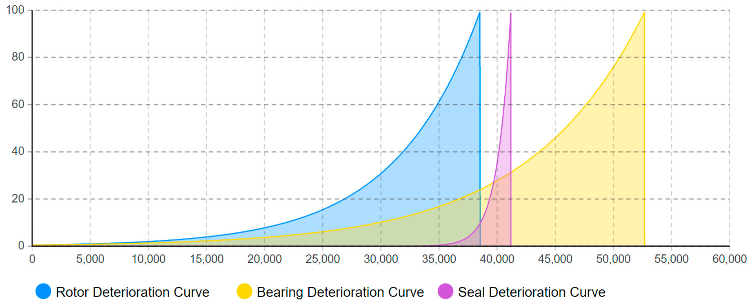
The final use case scenario, Scenario 5, is dedicated to the deterioration modeling of the components associated with the case study, i.e., rotor, bearing, and seal. Modeling component deterioration is required to highlight the capabilities of implementing an intelligent maintenance management system, i.e., levels of detection, diagnosis, and prognosis [
16]. This paper develops individual loading equations of the components of interest, based on the plot presented by Calixto [
25]. Since Calixto only represents the deterioration curves and not the specific deterioration equations, the associated loading equations presented in
Table 8 are replications.
The individual loading equations developed are then incorporated into the “Loading model” (shown in
Figure 5) and are simulated and optimized to fit the designed lifetime presented by Calixto [
25] using Anylogic, as depicted in
Figure 6. As seen, the deterioration curves highlight the entire deterioration process from when the specific component starts operating until a fault is present at the designed lifetime. The deterioration curves also demonstrate that the component deterioration propagates differently. Clearly, this affects the opportunities of detecting, diagnosing, and predicting the future behavior of the associated component deterioration process. For example, the deterioration of the seal appears with a steeper slope in comparison to the two other components, which thus reduces the opportunities of performing intelligent maintenance as it is more difficult to detect and predict the occurrence of seal deterioration. In contrast, the deterioration curve of bearing introduces the gentlest slope, which increases the opportunities to perform intelligent maintenance as it is possible to detect and predict the occurrence of bearing deterioration at an early stage.
It is important to highlight that this research adopts a detection and prediction level of 70% for Scenario 5. The main justification of this selection is based on recommendations from the literature [
31] and experts in the field.
2.4. Steps 5 and 6: Verification, Validation, and Visualization
The fifth step in the simulation modeling methodology concerns the verification and validation of the simulation. In this case, all the applied data, i.e., operation and maintenance including condition monitoring (
Figure 2), scheduled maintenance plans (
Figure 3), and experienced failures and following corrective maintenance (
Figure 4) including failure modes, failure rates, and MTTR values are extracted from the notification system of the case company and incorporated into the computational model. The applied data is also validated through several discussions with engineers and experts in the field represented by the case company and stakeholders for verification and validation purposes to attain a correct description of the case study, to increase the reliability of the results obtained from the simulations. In final, to improve the reliability of the simulations even more, similar data, i.e., failure modes, failure rates, and MTTR values are extracted from the well-known OREDA database [
17] and also compared to the real-time data extracted from the notification system of the case company.
The computational model is considered generic in that sense the future adopter can fit the model to their own purposes. In more detail, this means that the future adopters can replace the components with the ones of interest. Furthermore, the associated scheduled maintenance causing operational unavailability and thereby representing opportunistic maintenance intervals, and corrective maintenance data including failure modes, failure rates, and MTTR values can be replaced. This means that all data can be replaced by the ones of interest, however, the logic of the model must be kept, i.e., triggers and equations.
4. Discussion and Validation
4.1. Data Collection
Data in terms of scheduled maintenance plans and experienced corrective maintenance including failure modes, failure rates, and MTTR values were extracted from the notification system of the case company and incorporated into the computational model. In addition, several discussions with engineers have been conducted to attain a correct description and understanding of the case study and its data. In final, to improve the reliability of the simulations, data including failure modes, failure rates, and MTTR values were extracted from the OREDA database and compared with the experienced case study data.
4.2. Human Factors in Notification Processes
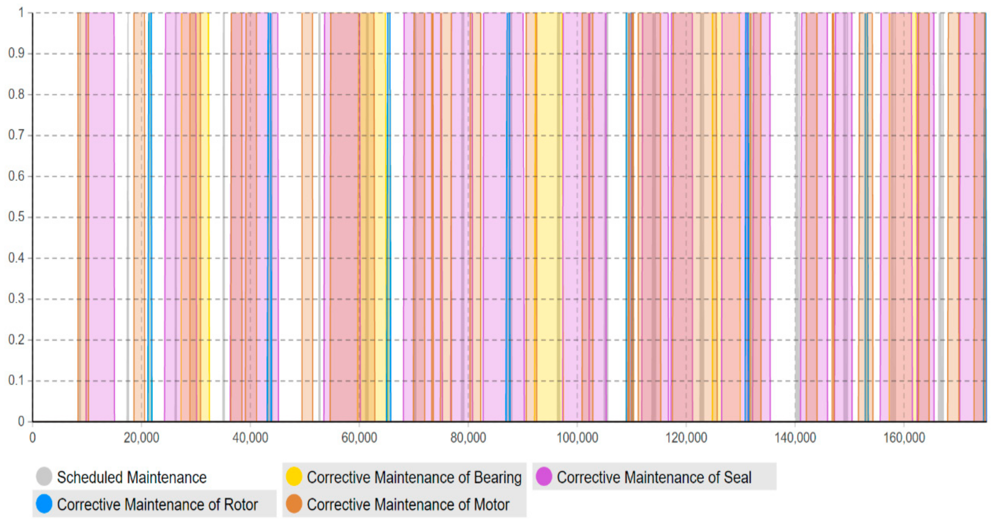
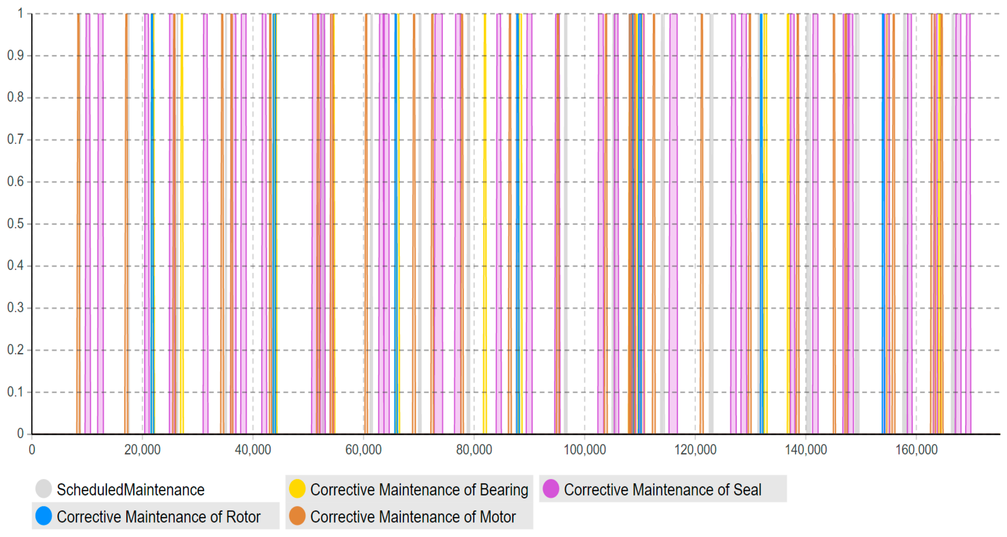
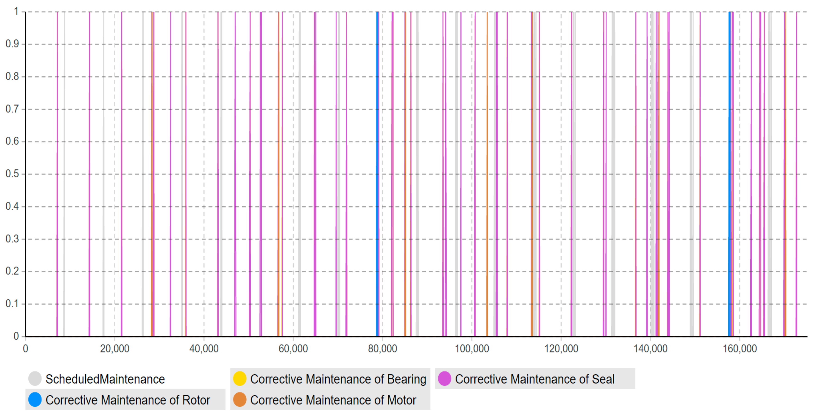
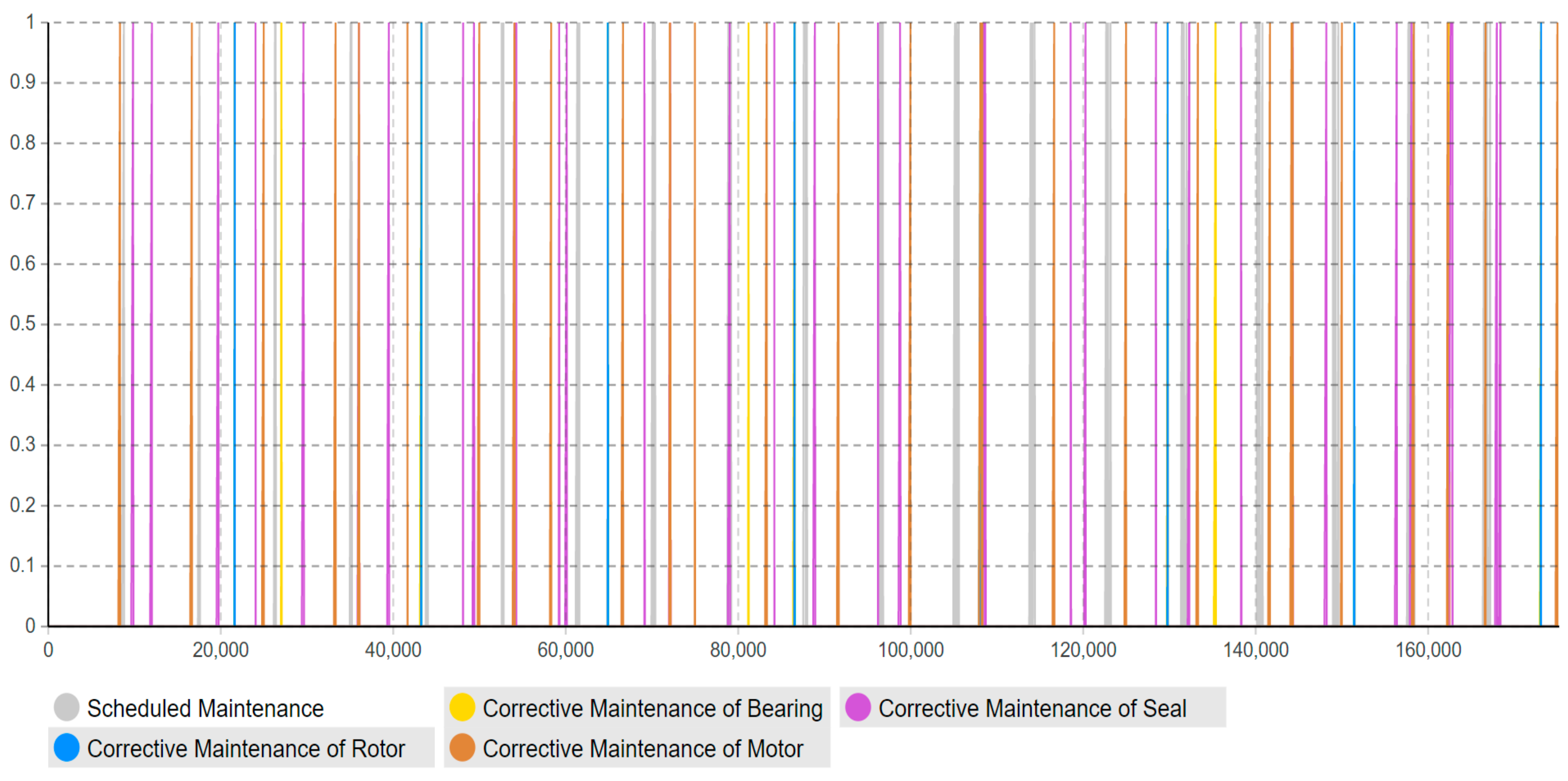
The data collection process of the empiric case study data became a lot more time-consuming than first anticipated. Its sole reason is traced back to human factors present in the notification processes that evidentially reduced the quality of the data significantly. This issue is clearly demonstrated by the simulated results. Use case Scenarios 1, 2, and 4 include the same failure rates extracted from the case study but with different MTTR values. In more detail, Scenario 1 includes MTTR values as presented in the notification process, Scenario 2 includes manipulated MTTR values considered as unreasonable extremes in the previous scenario, and Scenario 4 includes MTTR values extracted from the OREDA database [
17]. Therefore, the volatile changes in operational behavior and significant differences in maintenance workload between these three scenarios are solely traced back to the MTTR values. Respectively, the maintenance workload (in hours) devoted to corrective maintenance for Scenarios 1, 2, and 4 are 107,700, 44,055, and 3262 with associated operational availabilities of 37.756, 73.384, and 95.750%.
From the authors’ perspective, the main issue of incorporating human factors in the notification processes is traced back to the maintenance personnel’s opportunity of developing a notification that is solely based on subjective perceptions, without any associated requirements concerning the level of details of the individual notifications. Following this, the simulated results also justify why the O&G companies keep using the OREDA database [
17] and not their own empiric data in connection with analysis related to, e.g., technical integrity and risk. However, it is a paradox that case-specific data do not express the case of interest the best. Therefore, for the future, it shall be recommended that the notification processes avoid incorporating human factors, at least, reducing its impact by making the notification process (partial) automatic or based on a templated questionary with pre-defined alternatives the maintenance personnel is required to answer before the notification is considered as complete.
At last, it is also important to emphasize that the failure data originating from the case study includes several components of one component, i.e., rotor, bearing, and seal. However, due to difficulties in differentiating between these specific components, the failure rates presented in this research do not take into consideration the number of each component. Illustratively, this means that this research estimates one failure rate composing all the failures associated with one type of component, without taking its population into consideration. Therefore, the failure rate assumes that failure of, for instance, one bearing, results in failure of all the bearings present in the case study at the same time.
4.3. Intelligent Maintenance (Scenario 5) vs. Corrective Use Case (Scenario 4)
The final results of this research clearly demonstrate tempting lifetime benefits during 20 years of operation. In comparison, the intelligent maintenance system is expected to improve the operational availability by 0.268% by replacing 2.721% ((4183/16181) − (3724/16101) = 2.721%) of the corrective maintenance workload with intelligent maintenance. In workload, it equals replacing 459 h of corrective maintenance which corresponds to a reduction of 11% ((4183 − 3724)/4183 = 11%) of the total corrective maintenance workload. Specifically, the intelligent maintenance system reduced the unintended corrective maintenance visits by 20 (26.316%), whereas a reduction of 5 (62.500%), 8 (61.538%), and 7 (24.138%) corrective maintenance visits are traced back to the rotor, bearing, and seal, respectively. Following, these 20 corrective maintenance events were replaced by intelligent maintenance which leverages the PdM capabilities into opportunistic maintenance intervals and thereby does not affect the operational availability.
4.4. Additional Lifetime Benefits of Intelligent Maintenance in Industry 4.0
There exist some aspects that can improve the lifetime benefits even more, which are not presented in this paper. First, reducing component loading to extend the remaining useful life estimation and by this reach an opportunistic maintenance interval that was initially not reachable. Second, the expected improvements in terms of maintenance performance and in reducing the level or repair. In fact, enabling detecting, diagnosing, and predicting the future behavior of component deterioration is expected to support developing detailed work orders and ensure that the necessary spare parts and resources are available at the time of intelligent maintenance. However, since the proposed intelligent maintenance system remains to be implemented, it is difficult to justify the realistic values of these improvements. Nevertheless, this can be implemented in a future stage after obtaining operational experience post the implementation, which is traceable back to the MTTR values presented in, e.g., the notification system.
4.5. Intelligent Maintenance vs. Maintenance 4.0
There exists a large number of terminologies that are supposed to define maintenance management in Industry 4.0 such as, e-Maintenance [
32], intelligent maintenance [
33,
34], smart maintenance [
35], deep digital maintenance [
36], and Maintenance 4.0 [
37]. However, this paper adopts the terminology of intelligent maintenance, which intentionally differs from other terminologies e.g., smart maintenance [
35], e-maintenance [
32], as the focus is not primarily based on data analysis i.e., detection, diagnosis, and prognosis. However, this paper extends the scope to also consider enterprise-level data e.g., spare part management, seasonal loadings, available resources, in order to provide a solid foundation for the maintenance decision management that shall ensure that the right maintenance takes place at the right time. Furthermore, the term Maintenance 4.0 might bring the question about other technologies like robotics, augmented reality, additive manufacturing, i.e., 3D printed spare parts.
4.6. From a Case-Specific Computational Model into a Generic Computational Model
Although this paper develops a computational model based on a case study and presents simulated results associated with the case-specific data, it is important to emphasize that the computational model is easily converted to other cases of interest as the paper adopts a generic research methodology. To do so, the future adopter solely needs to incorporate general information from the specific case of interest including failure modes, scheduled maintenance plans representing opportunistic maintenance intervals, failure rates, and MTTR values. In this context, the authors recommend future adopters apply the PdM assessment matrix [
16] to identify associated failure modes, failure mechanisms, and to determine the levels of detection, diagnosis, and prognosis associated with the specific condition monitoring system included in the case of interest. The only requirement is that the computational model presented in this research retains its model structure, triggers, and logic.
5. Conclusions
The simulated results obtained from the multi-method computational model developed in this paper clearly show the ability to estimate the lifetime benefits of applying several maintenance strategies (preventive, corrective, predictive, and opportunistic) on an industrial asset. Simulating preventive, corrective, and opportunistic maintenance is already done in literature (discussed in the introduction). The novelty and scientific contribution of this computational model is mainly traced back to its ability to (1) simulate and estimate CBM and PdM behaviors and their lifetime benefits, (2) leverage PdM into opportunistic maintenance in terms of intelligent maintenance, and (3) estimate and quantify the maintenance workload and determine the specific maintenance event timeline.
Simulating CBM and PdM behaviors was enabled by the deterioration timeline concept where a deterioration curve based on loading profile is simulated, and detection and prediction levels are incorporated. In fact, most of the existing simulation models utilize the failure timeline concept generating pulse train curve, which is useless in order to incorporate detection and prediction levels. It can be concluded that the load-based deterioration curve, shown in
Figure 6, is an effective concept to enable the lifetime benefits estimation of CBM and PdM. Definitely, this is a challenging issue since there are some components that either have an unknown deterioration curve or random failure curve (undetectable or unpredictable). For example, only deterioration curves for the rotor, bearing, and seal were available for this case study.
The developed multi-method simulation model enables leveraging PdM capabilities into potential opportunistic intervals in terms of intelligent maintenance. It enables studying if the designed PdM specifications support gaining the lifetime benefits by utilizing potential opportunistic intervals or not. It is a core aspect to consider whether the maintenance system is intelligent or not. Intelligence in this context means that the maintenance management system is able to use detection, prediction, and scheduling analytics to optimize the maintenance events and utilize opportunistic intervals. It can be concluded based on
Table 11 that the corrective maintenance events were reduced by earlier detection level or farther predictive horizon, e.g., detection and prediction at 60% of a component lifetime offers increased lifetime benefits (72.727% reduction in corrective maintenance events related to bearing, seal, and rotor) compared with the corrective maintenance reduction percent (27.272%) at 90% of asset lifetime. Please note that PdM at 90% of a component lifetime is capable of detecting sudden failures before their occurrence, however, the opportunistic intervals will not be utilized due to the short time notice. It is important to enable maintenance engineers to determine the optimal technical specifications, i.e., detection and predictive capabilities, and be able to revise and optimize such technical specifications at the design phase.
Moreover, this model has adopted the “timeline” concept to estimate and quantify the maintenance workload amount (how much) in the specific timeline (when), rather than just the accumulated workload amount for the entire lifetime. As shown in
Figure 13,
Figure 14,
Figure 15,
Figure 16 and
Figure 17, the corrective maintenance events are time-specific. The timeline concept is required and highly useful for maintenance scheduling purposes, especially, to utilize opportunistic maintenance (based on usage or season) in an intelligent manner. Regarding the quantification of lifetime benefits of intelligent maintenance, the developed simulation model mainly covers two aspects of lifetime benefits (1) operational behavior and (2) maintenance workload. For example, the intelligent maintenance system for this case study at 70% detection and prediction level (able to detect failures after 70% of the asset lifetime), is estimated to improve the operational availability by 0.268% (shown in
Table 9) and reduce the maintenance workload devoted to corrective maintenance by 459 h (based on
Table 10) which equals 11% during 20 years of operation. Furthermore, intelligent maintenance management is also estimated to reduce the scheduled maintenance workload (that leads to downtime) by 0.339% ((3262–3251)/3262 = 0.339%), however, it will increase the scheduled maintenance workload (that does not lead to downtime) by 0.333% ((8765–8736)/8736 = 0.333%).
In summary, the developed simulation model has shown the ability to estimate the lifetime benefits in terms of operational availability and its reduction of corrective maintenance workload. The authors claim that the lifetime benefits of intelligent maintenance will become even greater than what is anticipated in this paper, once other lifetime benefit aspects, which are not covered by this research, are considered. This includes lifetime benefit aspects, i.e., increasing both number and levels of detection and prediction of failure modes, improving maintenance performance by reducing the level of repair, reducing scheduled maintenance workload, enhancing asset performance, lifetime extension measures for tactical and strategical decisions, and health, safety, and environmental issues, and capital allocations. Definitely, the simulation model shall be developed further to estimate all these lifetime benefits.
The structure of the developed simulation model is valid as it was extracted and validated based on experts from the case study. The structure illustrated in the statechart (
Figure 1) represents (1) maintenance policy type (corrective and scheduled) and decision making (trigger and condition to get notifications), and (2) failure modes. The statechart represents how the system in this specific case company generates failure or maintenance notification and how it can trigger maintenance events. It is important to highlight that this state chart is valid for other O&G companies operating in the Norwegian Continental Shelf. Regarding the failure modes, the statechart considers all standardized failure modes (based on ISO14224) matching the well-known OREDA database. Thus, the authors claim that the presented state chart is generic for O&G compressors, while the methodology is generic for any equipment of interest.
The model inputs are also analyzed in a pragmatic manner, i.e., several data sources (historical data records from the case study, OREDA, and physics-based deterioration curves). The historical data related to failure and corrective maintenance events provide valid and reliable failure rates and MTTR values, as long as the incomplete data (e.g., maintenance ending date) are manipulated. Failure rates and MTTR values extracted from the OREDA data are well known and accepted in the Norwegian O&G industry as a valid and reliable source of information. The deterioration curves extracted from Calixto [
25] are also valid and reliable curves.
The model outputs, i.e., simulated behaviors and estimated key performance indicators have been validated by comparing them to real-world data (case study historical data). The simulated availability and corrective maintenance timelines were validated with case company experts and numbers originating from case study literature [
1]. It can be concluded that the computational model is quite effective in terms of computation time. This simulation model uses hours as time-unit, which means it simulates failure rate per hour and checks all conditions (triggers) every time unit. It takes on average around 48 h (where a “normal computer” is used) to provide results at equipment level, i.e., compressor. However, for future simulations, the authors recommend days as time-unit, especially once the model is scaled up to system-level, i.e., compression section and plant-level. In addition, it is recommended that the failure rates are simulated based on years instead of hours.
The computational model is easily generalized to fit any condition monitoring system of interest. In this context, future adopters solely need to incorporate general information from the specific case of interest, i.e., failure modes, scheduled maintenance representing opportunistic maintenance intervals, failure rates, and MTTR values. In fact, the authors recommend applying the PdM assessment matrix [
16] to identify associated failure modes, failure mechanisms, and to determine the levels of detection, diagnosis, and prognosis associated with the specific condition monitoring included in the case of interest. The only requirement is that the computational model presented in this retains its model structure, triggers, and logic.
Regarding scenarios (
Table 6), it is recommended to use Scenario 4 for further simulation as the failure rates are quite reliable in the case study historical data, while the MTTR values presented by the OREDA database are most reliable and accurate (presented in hours in comparison to the case study presenting the MTTR in days).
At last, besides the quantifiable results presented in this research, it also addresses the sensitiveness and challenges concerning incorporating human factors into the failure notification processes. From the authors’ perspective, the main issue of incorporating the human factors in the notification processes is traced back to the maintenance personnel’s opportunity of developing a notification that is solely based on subjective perceptions, without any associated requirements to the level of detail for the individual notification. Following this, the simulated results also justify why O&G companies keep using the OREDA database [
17] and not the company’s own empiric data in connection with analysis related to, e.g., technical integrity and risk. Therefore, for the future, it shall also be recommended that the notification processes avoid incorporating human factors, at least, reducing its impact by making the notification process (partially) automatic or based on a templated questionary with pre-defined alternatives that the maintenance personnel are required to answer before the notification is considered as complete.


