Hybrid Optimization Method for Correcting Synchronization Errors in Tapping Center Machines

Abstract

A hybrid method is proposed for optimizing rigid tapping parameters and reducing synchronization errors in Computer Numerical Control (CNC) machines. The proposed method integrates uniform design (UD), regression analysis, Taguchi method, and fractional-order particle swarm optimizer (FPSO) to optimize rigid tapping parameters. Rigid tapping parameters were laid out in a 28-level uniform layout for the experiments in this study. Since the UD method provided a layout with uniform dispersion in the experimental space, the UD method’s uniform layout provided iconic experimental points. Next, the 28-level uniform layout results and regression analysis results were used to obtain significant parameters and a regression function. To obtain the parameter values from the regression function, FPSO was selected because its diversity and algorithmic effectiveness are enhanced compared with PSO. The experimental results indicated that the proposed method could obtain suitable parameter values. The best parameter combination in FPSO yielded the best results in comparisons of the non-systematic method. Next, the best parameter combination was used to optimize actual CNC machining tools during the factory commissioning process. From the commissioning process perspective, the proposed method rapidly and accurately minimizes synchronization error from 23 pulses to 18 pulses and processing time from 20.8 s to 20 s. In conclusion, the proposed method reduced the time needed to tune factory parameters for CNC machining tools and increased machining precision and decreased synchronization errors.

1. Introduction

Manufacturing internally threaded mechanical parts, particularly parts with numerous threads, requires high machining precision. Fabrication of threads using high-precision molds is usually the final step in the manufacturing process. Therefore, manufacturers require a reliable method of maintaining high quality in machining internal threads, especially in mass-produced mechanical components with internal threads. Tapping accuracy largely depends on whether the movement of the feed of the tapping axis is well synchronized with the rotation of the spindle during the tapping cycle. The observed index of the tapping axis feed to spindle rotation is the synchronization error. Therefore, to obtain a high-precision internal thread by rigid tapping, the goal is to minimize synchronization error.

For servo parameter commissioning, Lee et al. [1] proposed an iterative measurement and contour performance simulation. Servo parameters were adjusted to reduce contour error, and the Kreuz–Gitter–Meβsystem (KGM) method was used to verify the contour’s accuracy. Yeh et al. [2] proposed “learning automata,” an automatic parameter adjustment method for improving parameter convergence and improving efficiency in adjusting control parameters. To optimize the synchronous motion between the spindle and the tap-ping axis, Yeh et al. [3] proposed several linear and nonlinear control design techniques for improving control performance and synchronization, including (1) Cross-coupling control, (2) Nonlinear friction compensation, and (3) Interference observation. Servo gain was optimized by the command control method. The authors achieved synchronization accuracy within 10 ums at a spindle speed of 6000 rpm by applying these techniques. Lu et al. [4] used a fuzzy adaptive proportional–integral–derivative (PID) controller to control Computer Numerical Control (CNC) machine tools used in rigid tapping. The proposed control method can be performed without establishing a controlled object, and the online PID controllable parameters are automatically adjusted by the fuzzy inference method. In another study, Ishizaki et al. [5] proposed a cross-coupled controller for accurately synchronizing the motion of a servo system driven by dual motors. The proposed cross-coupled controller compensates for differential positioning errors between dual servo drives by modifying reference positions and speed commands. Biris et al. [6] performed experiments to compare the effectiveness of eliminating positioning and contour errors. The authors also proposed an adjustment method based on a mathematical model and evaluated its performance in reducing positioning and contour errors in CNC machine tools. Chen et al. [7] proposed an iterative learning control (ILC) algorithm for reducing synchronization error in rigid tapping.

In recent years, additive manufacturing (AM) technology has been proposed to be suitable for manufacturing critical components. Additive manufacturing is completely different from traditional subtractive processing. In contrast, additive manufacturing uses polymer, metal, or ceramic material spray stacking to construct a 3D shapes method that can quickly and flexibly produce a small number of diverse products, significantly reducing the time from the design stage to mass production of the products and considerably improving the utilization rate of materials [8,9,10,11,12]. At present, additive manufacturing can be used to produce energy, aerospace, or biomedical parts, providing high-strength and lightweight products. The machine tools manufacturer MAZAK’s hybrid multi-objective machine tool type can perform laser additive manufacturing and 5-axis machining processes on machine tools, demonstrating the possibilities and characteristics of future advanced techniques [13].

The learning control modifies the z-axis and the spindle commands to optimize synchronicity between z-axis output responses and the spindle. Their experiments revealed that 10 runs of the ILC algorithm reduced synchronization error from 0.26 mm to 2.6 × 10⁻¹³. That is, the use of ILC learning control can substantially reduce synchronization error. Chen et al. [14] proposed intelligent computer-aided process planning (i-CAPP). When the machining process’s complexity increases, i-CAPP’s Integration intelligence function works together with the domain expert’s procedure. Ma et al. [15] accord the coupling between the radial and axial vibrations and the dynamic cutting forces modeled along the tapping path. The radial and axial chatter stability is separately predicted in the frequency domain for the tapping process’s stability.

In the past, when the machining process was executed in the factory, the teeth or the tapping tools occasionally broke when the tapping speed was different. Usually, it was necessary to wait for the equipment manufacturer to inspect the equipment to obtain the best parameters. The current study developed a novel method of adjusting rigid tapping electrical control parameters and explored the effects of the adjusted parameters on thread quality obtained by tapping in internally threaded parts. The proposed method combines uniform design (UD) [16,17,18,19], regression analysis [20,21,22,23], fractional-order particle swarm optimizer (FPSO) [24,25,26,27,28], and the Taguchi method [29,30,31,32,33,34,35,36] to analyze the effects of rigid tapping parameters on thread quality and to determine the key parameters and the optimal parameter values. Application of the proposed method in an actual factory process verified its effectiveness for improving thread tapping quality. Through the method provided in this article, the processing industry can get the minimum error parameter combination at different tapping speeds through experiments to avoid breaking the tool when rigid tapping is performed at the end of the processing process and causing damage to the workpiece.

This paper is organized as follows. The problem considered in this study is briefly described in Section 2. Section 3 briefly discusses relevant methods, including UD, regression analysis, FPSO, and the Taguchi method. Section 4 presents and discusses the experimental and simulation results. Finally, Section 5 concludes the study.

2. Problem Description

Machining internal threads is an essential process in mechanical parts manufacturing in various industries. For example, numerous internally threaded holes are required to manufacture printed circuit boards (PCBs) in the computer, communications, and consumer-electronics (3C) electronics industry and manufacture mobile phone cases in the mold industry. Holes are typically threaded in a late stage of the manufacturing process. Poorly threaded holes can severely diminish the manufactured part’s quality and performance; therefore, manufacturers require a fast and reliable method for tapping internally threaded holes.

Tapping can be classified as floating or rigid. Each method uses a different tool clamping device, so each method has different synchronization requirements for the spindle and the tapping axis. Floating tapping was developed to solve the problem of synchronization between the spindle and the tapping axis. In floating tapping, the tap-ping tool is clamped in an elastic chuck. The advantage of floating tapping is that tapping can be achieved without complex control theory. The disadvantage, however, is that an excessively high tapping speed causes severe vibration resulting in imprecise tapping and/or disordered or broken teeth. In rigid tapping, a tap collet is typically used to clamp the tapping tool, which provides more precise teeth and enables a more efficient tapping speed than floating tapping. Rigid tapping is also much faster than floating tap-ping. However, synchronization between the spindle and the tapping axis must be exact. Even a slight difference can cause a breakage of the tool. Therefore, accurate synchronization of the spindle and tapping axis is essential. Most research in rigid tap-ping control has focused on minimizing the synchronization error between the tapping axis movement and the spindle to obtain internal threads with high quality and accuracy.

To obtain the required screw pitch specifications in a rigid tapping process, the tapping axis and the spindle must be adjusted to meet the required combination of spindle speed and feed rate of the tapping axis. The relationships can be formulated as in Equation (1)

P = F/S

(1)

where P is the thread pitch (unit: mm), F is the feed rate of the tapping axis (unit: mm/min), and S is the spindle speed (RPM).

In a rigid tapping procedure, the spindle speed and tapping axis feed rate must maintain a certain proportional relationship according to the required pitch specifications. Because pitch P depends on the scale of spindle speed and feed rate of the feed axis, if spindle speed and feed rate of feed axis do not match, it causes synchronization error which is too large and pitch P, not precision. Therefore, the controller has a command-type compensation architecture, and the controller simultaneously commands the spindle and the tapping axis and compensates for positioning errors.

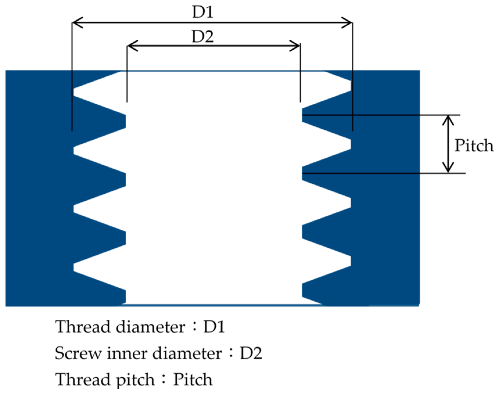
Additionally, the FANUC 31iMA controller used in this experiment is that the control method in which the tapping axis follows the spindle identifies synchronization errors between the spindle and the tapping axis. Figure 1 shows that synchronization error is an essential indicator in rigid tapping because it affects internal threads’ shape and precision.

3. Related Research

This section briefly describes the methods applied in the modeling process, including the UD method [16,17,18,19], regression analysis [20,21,22,23], FPSO [24,25,26,27,28], and Taguchi method [29,30,31,32,33,34,35,36].

3.1. Uniform Design and Regression Analysis

The UD method proposed by Fang and Wang [17,18] was used to design and plan experiments in which the test points were evenly distributed within the test range. A uniform layout is expressed as U_n(n^s), where U is the uniform layout, n is the level number, and s is the factor number.

Table 1. The U₆(6⁶) uniform layout.

U6(66)	1	2	3	4	5	6
1	1	2	3	4	5	6
2	2	3	6	1	3	5
3	3	6	2	5	1	4
4	4	1	5	2	6	3
5	5	3	1	6	4	2
6	6	5	4	3	2	1

shows the distribution of a U₆(6⁶) uniform layout.

In the UD method, data collected in experiments were used for model building, and data analysis was performed using regression analysis. Regression analysis is a statistical method for analyzing relationships between input variables and output variables. Its main purposes are understanding the relationships among independent variables and dependent variables and then building a mathematical model for predicting dependent variables. Depending on the complexity, a regression analysis can be classified as simple regression and multiple regression. Simple regression uses a single independent variable to predict a dependent variable, and multiple regression explores how a dependent variable is related to multiple independent variables.

The unary linear regression equation expresses the relationship between a dependent variable and an independent variable:

Y = β₀ + β_1×1 + ε

(2)

where β₀ is a constant, β₁ is a regression coefficient, and ε is an error.

A multiple linear regression equation expresses the relationship of a dependent variable to multiple independent variables:

Y = β₀ + β_1×1 + β_2×2 + β_3×3 + … + β_m×m + ε

(3)

where β₀ is a constant, β₁, β₂, β₃, …, β_m is a regression coefficient, and ε is an error.

Regression analysis is often used for the interpretation of experimental data and prediction. For interpretation, the regression equation was calculated from the obtained experimental data. The equation was then used to determine the contribution of each independent variable to the dependent variable. A common application of regression analysis is determining the significance of the independent variable to the dependent variable. Since the regression equation is linear, regression analysis can be used for prediction, i.e., to estimate how an independent variable will change a dependent variable. That is, after regression analysis, a regression model is used to predict a future change in a dependent variable, it can be used to determine how to compensate or respond to the change.

3.2. Fractional-Order Particle Swarm Optimization (FPSO)

The FPSO was first proposed by Solteiro Pires et al. [27] and was derived from PSO by introducing the Grünwald–Letnikov fractional-order derivative to enhance its diversity and algorithmic effectiveness. The PSO algorithm [37,38,39,40,41] was inspired by the group behavior of foraging birds and seeks the best solution in the solution space by maximizing or minimizing fitness value, which is analogous to the process in which foraging birds maximize the amount of food they consume. Evolution of position and evolution of speed occur as the optimal parameters for position and speed are updated after each iteration. The calculation formula for PSO is as follows:

V_i(k + 1) = ω∙V_i(k) + c₁∙r₁∙ (P_i^l(k) − p_i(k)) + c₂∙r₂∙ (P^g(k) − p_i(k))

(4)

p_i(k + 1) = p_i(k) + V_i(k + 1)

(5)

where i = 1, 2, …, m (m is the number of particles); k is the number of iterations; w is the inertial weight; V is the velocity; c₁ and c₂ are individual and group parameters, respectively; p_i(k) is the position vector; P_i^l(k) is the best local solution in the current iteration; P^g(k) is the best global solution in the current iteration, and r₁ and r₂ are random numbers from 0 to 1.

Recently, many studies enhanced the performance and effectiveness of PSO, including adjusting the strategies [42,43], particle grouping [44,45,46], inertia weights [47,48,49], and other optimization techniques [50,51,52,53]. However, PSO has its main drawbacks, such as lack of robustness and tendency to fall into the local optimum. Additionally, the fractional-order derivative describes the real world more than the integer-order one. Therefore, Solteiro Pires et al. [27] involved the fractional-order derivative in PSO to improve the performance and effectiveness, called FPSO. After that, Gao et al. [28] took a nonlinear time-varying inertia weight in FODPSO (Fractional-order Darwinian PSO) to improve. In this paper, the inertial weight was applied to FPSO, and the calculation formula is as follows:

V_i(k + 1) = ω∙V_i(k) + c₁∙r₁∙ (P_i^l(k) − λ∙p_i(k) − λ/2∙(1 − λ)∙p_i(k − 1) − λ/6∙(1 − λ)∙(2 − λ)∙p_i(k − 2) − λ/24∙(1 −
λ)∙(2 − λ)∙(3 − λ)∙p_i(k − 3)) + c₂∙r₂∙ (P^g(k) − p_i(k))

(6)

p_i(k + 1) = p_i(k) + V_i(k + 1)

(7)

where λ is the fractional order of the derivative.

3.3. Taguchi Method

The purpose of the Taguchi method [29,30,31,32,33,34,35,36] is to achieve a design process in which product quality is stable and insensitive to various noises in the production process. In the product design process, functional relationships among quality, cost, and benefit are analyzed to maximize product quality and minimize production costs. A large number of design variables are studied in a small number of experiments. The best combination of design variables can be expressed by the orthogonal table and the signal-noise ratio (SNR). The basic concept of the Taguchi method is to maximize the performance index by using the orthogonal table to perform experiments. Using the orthogonal table reduces experiment time and increases convergence speed. In the Taguchi method, orthogonal arrays and SNR are tools used to optimize the design of engineering parameters in the experimental plan, to reduce variation in important quality characteristics, and to achieve the goal of total cost reduction.

Table 2. The L₉(3⁴) orthogonal array.

L9(34)	1	2	3	4
1	1	1	1	1
2	1	2	2	2
3	1	3	3	3
4	2	1	2	3
5	2	2	3	1
6	2	3	1	2
7	3	1	3	2
8	3	2	1	3
9	3	3	2	1

shows an example of an L₉(3⁴) orthogonal array that accommodates a maximum of 4 factors with 3 levels per factor.

The SNR was calculated for quality characteristics, and the goal of this study was the smaller, the better characteristics. The quality function characteristic Y is a non-negative value with a smaller-the-better characteristic; Y can be equal to zero. The SNR of the smaller-the better characteristic is defined as

$$SNR=-10lo{g}_{10}\frac{1}{n}{\displaystyle \sum }_{i=1}^n\left(Y_i^2\right)$$

(8)

4. Experimental Planning and Methods

Drilling and tapping processes are used in the manufacturing processes for diverse products ranging from cylinder engines in the automobile industry to mobile phone molds in the consumer electronics industry. Since the manufacture of these products often requires numerous drilling and tapping procedures, determining the parameter combination that provides the best tapping accuracy is needed to achieve high product quality in the post-process. This study’s objective was to find the parameter combination that minimizes rigid tapping synchronization error without increasing manufacturing time.

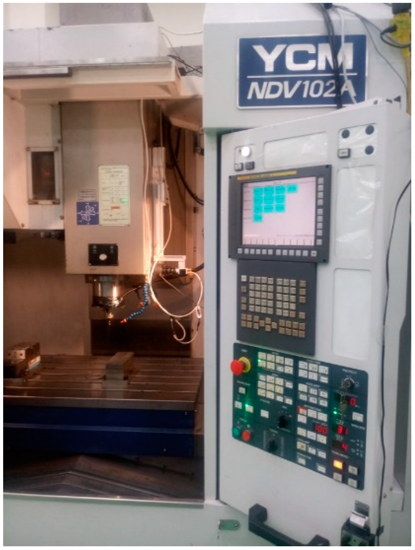
Figure 2 shows that the experiments were performed in an NDV series machine tool (Yeong-Chin machinery industries Co. Ltd., Taichung, Taiwan) with a FANUC 31iMA controller. The material used for the through-hole processing experiments was polymethyl methacrylate (PMMA) due to its high plasticity, high hardness, and low brittleness. The PMMA was considered an excellent experimental material because it enabled observation of broken or irregular cutters’ effects. Therefore, even a significant synchronization error would be unlikely to damage the tapping tool in the tapping axis. The phenomena of stripped thread or thread damage can still be observed in PMMA. An M6 × 1 tapping tool was used in the experiments. The cutting conditions were as follows. Spindle speed, tapping axis feed rate, and tapping depth were set to 3000 RPM, 3000 mm/min, and 50 mm, respectively. The experiment was performed five times at these settings. Figure 3 shows the processing path.

The experimental input was the factor that affected synchronization error, and the output was synchronization error. Input factors were factors that affected synchronization error, including feedforward speed coefficient (x₁, unit: 0.01%), rigid tapping speed loop proportional gain (x₂, unit: As), motor excitation delay time (x₃, unit: microsecond), rigid tapping speed loop integral gain (x₄, unit: microsecond)), feed position coefficient (x₅, unit: 0.01%) and tapping axis position gain (x₆, unit: 0.01s-1) [54,55,56,57]. These parameters were set on the FANUC controller system.

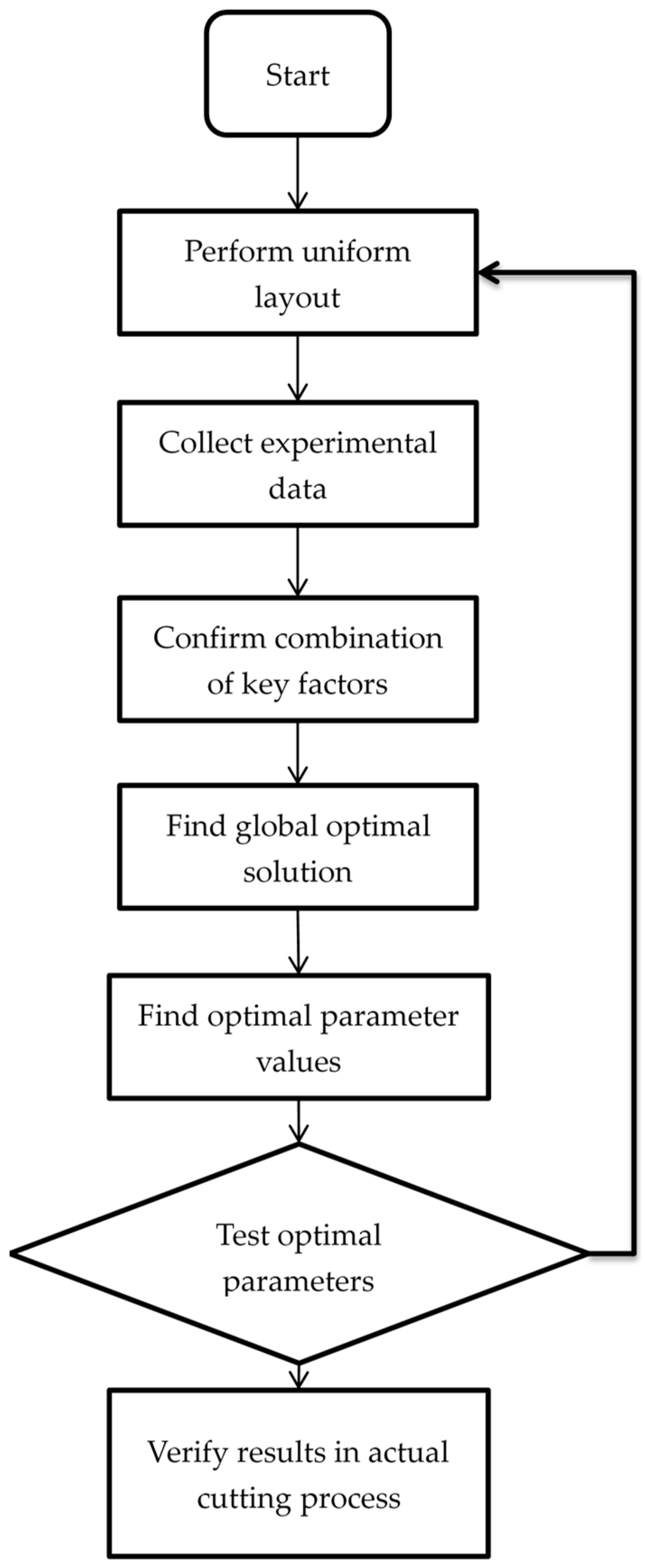
Figure 4 shows the experimental procedure. The uniform distribution characteristic of UD made each experimental combination meaningful, which substantially reduced the required number of experiments.

Table 3. The U *₂₈(28⁸) uniform layout.

U *28(288)	1	2	3	4	5	6	7	8
1	1	7	16	18	20	23	24	25
2	2	14	3	7	11	17	19	21
3	3	21	19	25	2	11	14	17
4	4	28	6	14	22	5	9	13
5	5	6	22	3	13	28	4	9
6	6	13	9	21	4	22	28	5
7	7	20	25	10	24	16	23	1
8	8	27	12	28	15	10	18	26
9	9	5	28	17	6	4	13	22
10	10	12	15	6	26	27	8	18
11	11	19	2	24	17	21	3	14
12	12	26	18	13	8	15	27	10
13	13	4	5	2	28	9	22	6
14	14	11	21	20	19	3	17	2
15	15	18	8	9	10	26	12	27
16	16	25	24	27	1	20	7	23
17	17	3	11	16	21	14	2	19
18	18	10	27	5	12	8	26	15
19	19	17	14	23	3	2	21	11
20	20	24	1	12	23	25	16	7
21	21	2	17	1	14	19	11	3
22	22	9	4	19	5	13	6	28
23	23	16	20	8	25	7	1	24
24	24	23	7	26	16	1	25	20
25	25	1	23	15	7	24	20	16
26	26	8	10	4	27	18	15	12
27	27	15	26	22	18	12	10	8
28	28	22	13	11	9	6	5	4

shows the U *₂₈ (288) uniform layout selected for this study’s experiments. First, input factors were entered in the U *₂₈ uniform layout. Synchronization error was the quality characteristic, and the response value was obtained by the-smaller-the-better characteristic.

Table 4. Table for selecting column numbers for the U *₂₈ uniform layout.

Number of Factors	Column
2	1 4
3	1 2 5
4	1 2 5 7
5	1 2 3 7 8
6	1 2 3 5 6 7
7	1 2 3 5 6 7 8

is the table for selecting column numbers according to the experiment number. Table 4 shows that columns 1–7 were used to construct the U *₂₈ (286) uniform layout, and

Table 5. The U *₂₈(28⁶) uniform layout implemented in this study.

U *28(288)	1	2	3	5	6	7
1	1	7	16	20	23	24
2	2	14	3	11	17	19
3	3	21	19	2	11	14
4	4	28	6	22	5	9
5	5	6	22	13	28	4
6	6	13	9	4	22	28
7	7	20	25	24	16	23
8	8	27	12	15	10	18
9	9	5	28	6	4	13
10	10	12	15	26	27	8
11	11	19	2	17	21	3
12	12	26	18	8	15	27
13	13	4	5	28	9	22
14	14	11	21	19	3	17
15	15	18	8	10	26	12
16	16	25	24	1	20	7
17	17	3	11	21	14	2
18	18	10	27	12	8	26
19	19	17	14	3	2	21
20	20	24	1	23	25	16
21	21	2	17	14	19	11
22	22	9	4	5	13	6
23	23	16	20	25	7	1
24	24	23	7	16	1	25
25	25	1	23	7	24	20
26	26	8	10	27	18	15
27	27	15	26	18	12	10
28	28	22	13	9	6	5

shows the resulting layout.

Table 6. Level-cut for rigid tapping factors.

Level	x1	x2	x3	x4	x5	x6
	Velocity Feed Forward Coefficient	Proportional Gain of Velocity Loop for Spindle in Servo Mode	Delay Time for Motor Excitation	Integral Gain of Velocity Loop for Spindle in Servo Mode	Advanced Feed Forward	Position Gain of Servo Axis for Rigid Tap
1	30	23	200	100	2500	3455
2	47	24	206	106	2778	3694
3	64	25	212	112	3056	3933
4	81	26	218	118	3334	4172
5	98	27	224	124	3612	4411
6	115	28	230	130	3890	4650
7	132	29	236	136	4168	4889
8	149	30	242	142	4446	5128
9	166	31	248	148	4724	5367
10	183	32	254	154	5002	5606
11	200	33	260	160	5280	5845
12	217	34	266	166	5558	6084
13	234	35	272	172	5836	6323
14	251	36	278	178	6114	6562
15	268	37	284	184	6392	6801
16	285	38	290	190	6670	7040
17	302	39	296	196	6948	7279
18	319	40	302	202	7226	7518
19	336	41	308	208	7504	7757
20	353	42	314	214	7782	7996
21	370	43	320	220	8060	8235
22	387	44	326	226	8338	8474
23	404	45	332	232	8616	8713
24	421	46	338	238	8894	8952
25	438	47	344	244	9172	9191
26	455	48	350	250	9450	9430
27	472	49	356	256	9728	9669
28	489	50	362	262	10,000	9908

shows the 28 levels for each factor. A CCD electronic image microscope was used to observe the results (thread pitch and workpiece shape) of the tapping experiments performed using the factor combinations in Table 5 and Table 6.

Table 7. The U *₂₈(28⁶) uniform layout implemented in this study.

No.	x1	x2	x3	x4	x5	x6
1	30	29	290	214	8616	8952
2	47	36	212	160	6948	7757
3	64	43	308	106	5280	6562
4	81	50	230	226	3612	5367
5	98	28	326	172	10,000	4172
6	115	35	248	118	8338	9908
7	132	42	344	238	6670	8713
8	149	49	266	184	5002	7518
9	166	27	362	130	3334	6323
10	183	34	284	250	9728	5128
11	200	41	206	196	8060	3933
12	217	48	302	142	6392	9669
13	234	26	224	262	4724	8474
14	251	33	320	208	3056	7279
15	268	40	242	154	9450	6084
16	285	47	338	100	7782	4889
17	302	25	260	220	6114	3694
18	319	32	356	166	4446	9430
19	336	39	278	112	2778	8235
20	353	46	200	232	9172	7040
21	370	24	296	178	7504	5845
22	387	31	218	124	5836	4650
23	404	38	314	224	4168	3455
24	421	45	236	190	9172	9191
25	438	23	332	136	8894	7996
26	455	30	254	256	7226	6801
27	472	37	350	202	5558	5606
28	489	44	272	148	3890	4411

displays the experimental results.

The rigid tapping command for the FANUC 31iMA controller used in the experiments was as follows:

M29 S__;

G84 X__Y__Z__R__F__K__;

where

M29 is the rigid tapping command,

S is the spindle speed, G84 is the right-hand thread tapping by M3 spindle rotation,

X, Y are the hole positions in the X- and Y-axes,

Z is the tapping depth from the R-plane to Z-depth,

R is the R plane position,

F is the tapping axis feed rate, and

K is the number of cycles.

The rigid tapping program was as follows:

G91 G94

N1

N2 M29 S3000

G84 Z-50.000 R-20.000 F3000.000 K5

G80

G04 X1.N999 G04 X1.

M99

Table 8. Results based on U *₂₈(28⁶) uniform layout.

No.	x1	x2	x3	x4	x5	x6	Sync Error
1	30	29	290	214	8616	8952	511.8
2	47	36	212	160	6948	7757	1303.2
3	64	43	308	106	5280	6562	2375.2
4	81	50	230	226	3612	5367	3909
5	98	28	326	172	10,000	4172	21.4
6	115	35	248	118	8338	9908	560
7	132	42	344	238	6670	8713	1270
8	149	49	266	184	5002	7518	2205.6
9	166	27	362	130	3334	6323	3479.8
10	183	34	284	250	9728	5128	178.4
11	200	41	206	196	8060	3933	1609
12	217	48	302	142	6392	9669	1247
13	234	26	224	262	4724	8474	2070
14	251	33	320	208	3056	7279	3161.2
15	268	40	242	154	9450	6084	310
16	285	47	338	100	7782	4889	1503
17	302	25	260	220	6114	3694	3423.4
18	319	32	356	166	4446	9430	1963.8
19	336	39	278	112	2778	8235	2915.6
20	353	46	200	232	9172	7040	409
21	370	24	296	178	7504	5845	1425.8
22	387	31	218	124	5836	4650	2651.2
23	404	38	314	224	4168	3455	5470.6
24	421	45	236	190	9172	9191	2719.4
25	438	23	332	136	8894	7996	488.8
26	455	30	254	256	7226	6801	1374.2
27	472	37	350	202	5558	5606	2627.4
28	489	44	272	148	3890	4411	4540.4

presents the results obtained by the U *₂₈(28⁶) uniform layout. Based on the regression analysis results and the experimental results in Table 8, the following regression equation was obtained:

y = 180.116319 − 3.143699x₂ − 0.023775x₆ + 0.008271x₂x₃ + 0.000115x₄x₅ + 0.000450x₂x₆ + 2.93 × 10⁻⁶
x₅x₆ − 4.18 × 10⁻⁷ x₃x₄x₅ −6.61 × 10⁻⁸ x₂x₅x₆

(9)

According to Equation (9), the key factors in synchronization error in rigid tapping are x₂ (rigid tapping speed loop proportional gain), x₃ (motor excitation delay time), x₄ (rigid tapping speed loop integral gain), x₅ (position feed coefficient) and x₆ (tapping axis position gain). Next, FPSO was used to find the global best combination of values for factors x₂, x₃, x₄, x₅, and x₆ and to find the global best output value. According to the FPSO results, the global best combination was (x₂, x₃, x₄, x₅, x₆) = (50, 360, 260, 9400, 9400), and the global best output value was 39.9329.

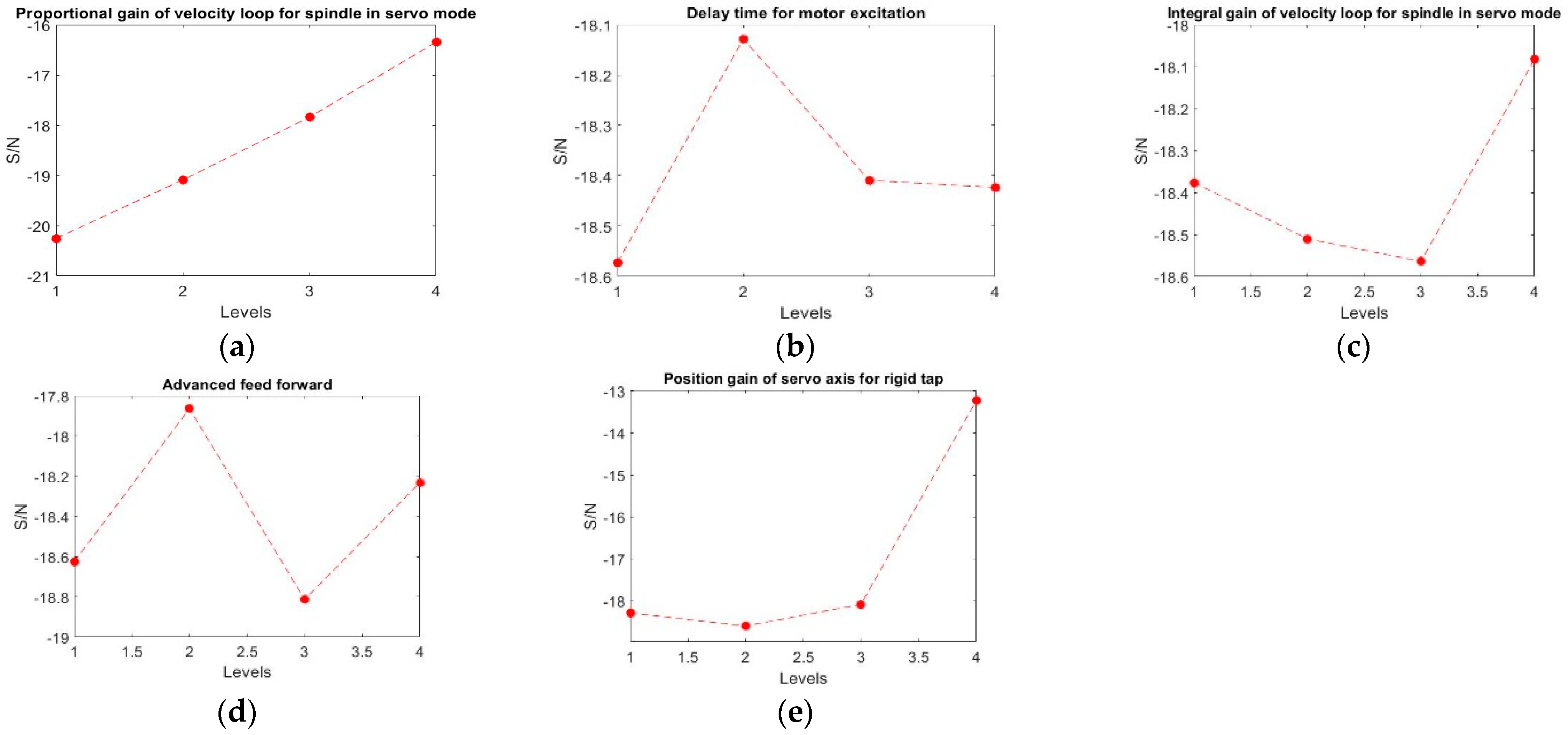
Next, the Taguchi method was used to verify the global best combination obtained by UD and FPSO.

Table 9. The L’₁₆(4⁵) orthogonal array.

No.	1	2	3	4	5
1	1	1	1	1	1
2	1	2	2	2	2
3	1	3	3	3	3
4	1	4	4	4	4
5	2	1	2	3	4
6	2	2	1	4	3
7	2	3	4	1	2
8	2	4	3	2	1
9	3	1	3	4	2
10	3	2	4	3	1
11	3	3	1	2	4
12	3	4	2	1	3
13	4	1	4	2	3
14	4	2	3	1	4
15	4	3	2	4	1
16	4	4	1	3	2

is the L’₁₆(4⁵) orthogonal array selected for this number of factors. Here, the levels of the L’₁₆(4⁵) orthogonal array were based on the global best combination obtained by UD and FPSO.

Table 10. The L’₁₆(4⁵) orthogonal array with level value for each factor.

No.	x2	x3	x4	x5	x6
1	40	350	245	6900	9600
2	45	355	250	7900	9700
3	50	360	255	8900	9800
4	55	365	260	9900	9900

shows the values for x₂, x₃, x₄, x₅, and x₆, and

Table 11. An L’₁₆(4⁵) orthogonal array with level value for each factor.

No.	x2	x3	x4	x5	x6
1	40	350	245	6900	9600
2	40	355	250	7900	9700
3	40	360	255	8900	9800
4	40	365	260	9900	9900
5	45	350	250	8900	9900
6	45	355	245	9900	9800
7	45	360	260	6900	9700
8	45	365	255	7900	9600
9	50	350	255	9900	9700
10	50	355	260	8900	9600
11	50	360	245	7900	9900
12	50	365	250	6900	9800
13	55	350	260	7900	9800
14	55	355	255	6900	9900
15	55	360	250	9900	9600
16	55	365	245	8900	9700

shows the factor combinations of L’₁₆(4⁵). The values in Table 11 were used to obtain the results shown in

Table 12. Results for L’₁₆(4⁵) orthogonal array.

No.	Factors					Results					Avg. 1	RMSD 2	H 3
	x2	x3	x4	x5	x6	1	2	3	4	5
1	40	350	245	6900	9600	10.5	10.5	11	11	10.5	10.7	114.55	−20.59
2	40	355	250	7900	9700	10	10	9.5	10	9.5	9.8	96.1	−19.8272
3	40	360	255	8900	9800	10.5	10	10.5	11	11.5	10.7	114.75	−20.5975
4	40	365	260	9900	9900	10	10.5	9.5	10	10	10	100.1	−20.0043
5	45	350	250	8900	9900	10	10	10	10	10	10	100	−20
6	45	355	245	9900	9800	8.5	8	8	8.5	8.5	8.3	68.95	−18.3853
7	45	360	260	6900	9700	9	9.5	9	9	9.5	9.2	84.7	−19.2788
8	45	365	255	7900	9600	9.5	8	8.5	8.5	8.5	8.6	74.2	−18.704
9	50	350	255	9900	9700	8	8.5	8.5	8	8	8.2	67.3	−18.2802
10	50	355	260	8900	9600	8	8	7	7.5	7.5	7.6	57.9	−17.6268
11	50	360	245	7900	9900	7.5	7.5	7.5	7.5	7.5	7.5	56.25	−17.5012
12	50	365	250	6900	9800	8	8	8	7.5	8	7.9	62.45	−17.9553
13	55	350	260	7900	9800	6	6	6	5.5	6	5.9	34.85	−15.422
14	55	355	255	6900	9900	6	6.5	7	7	7.5	6.8	46.5	−16.6745
15	55	360	250	9900	9600	6.5	6.5	6.5	6.5	6.5	6.5	42.25	−16.2583
16	55	365	245	8900	9700	7.5	6.5	6.5	6.5	6.5	6.7	45.05	−16.5369

¹ Avg: Average value in experiments. ² RMSD: Root-mean-square deviation. ³ η: Signal-to-noise ratio.

.

Table 13. Response table for L’₁₆(4⁵) orthogonal array results in Table 12.

No.	x2	x3	x4	x5	x6
1	−20.2548	−18.573	−18.3763	−18.6247	−18.2948
2	−19.0921	−18.1285	−18.5102	−17.8636	−18.6037
3	−17.8409	−18.409	−18.5641	−18.8132	−18.0901
4	−16.3459	−18.4231	−18.083	−18.232	−13.2319

and Figure 5 are the response table and figure, respectively, which show that the best combination of values for x₂, x₃, x₄, x₅, and x₆ was 55, 355, 260, 7900, and 9900, respectively.

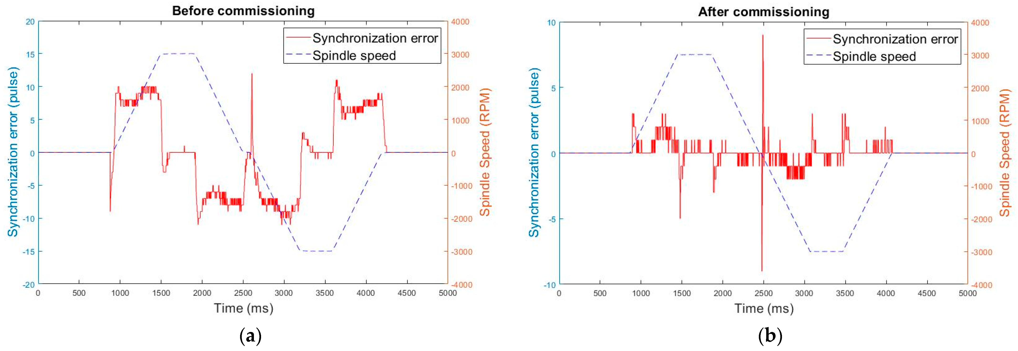
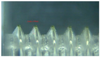
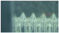
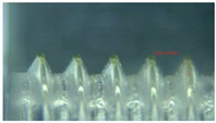
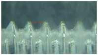
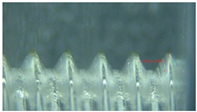
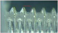
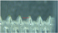
Figure 6 displays the rigid tapping errors obtained under the optimal parameter combination. Synchronization error was 23 pulses before adjustment and 18 pulses after adjustment. For verification, the simulation results and actual processing results were compared before and after optimization. The optimal combination was then used in an actual thread cutting process. After the process was performed five times, the bolt was cut in half with a face milling cutter, and the workpiece was placed under a CCD electronic image microscope to observe its shape and measure the pitch and appearance of the thread. The outer diameter (D1) and inner diameter (D2) of the thread were measured, and the difference between D1 and D2 was obtained.

Table 14. Difference between outer diameter (D1) and inner diameter (D2) before and after commissioning.

No.	Before Commissioning		After Commissioning
1		difference		difference
		0.96		1.06
2		difference		difference
		0.96		1.04
3		difference		difference
		0.98		1.04
4		difference		difference
		0.98		1.06
5		difference		difference
		0.98		1.04
	Average	0.972	Average	1.048

shows that a significant difference between D1 and D2 indicated that the screw teeth were well-shaped and that the potential for tooth collapse was minimal.

Conversely, a slight difference indicated poorly-shaped screw teeth and a high potential for tooth collapse. Screw thread pitch was also measured to determine whether disordered teeth had caused an excessive error during the same period. Table 14 shows that the proposed method obtained superior tapping results compared to the results obtained without optimizing rigid tapping electrical control parameters.

5. Conclusions

The proposed hybrid method for optimizing synchronization in rigid tapping was verified in an actual thread cutting process. Errors in synchronization of the spindle and the tapping axis were captured, and parameter values were adjusted for optimal synchronization.

Rigid tapping is easily performed when the CNC machine tool used for spiral tap-ping is operated at the expected speed and feed rate. However, high synchronization of motion is required to achieve a high-quality tap and avoid damage to the tapping tool and the workpiece. Therefore, the UD method proposed in this study integrated regression analysis, FPSO, and the Taguchi method to optimize rigid tapping parameters and obtained excellent tapping results.

For parameters x₂, x₃, x₄, x₅, x₆, the optimal combination of values was 55, 355, 260, 7900, and 9900, respectively. This combination reduced synchronization error from 23 pulses under the original parameters to 18 pulses, which was a 22% improvement in accuracy. The optimized combination also reduced processing time from 20,880 ms to 20,033 ms.

The method proposed in this study improves machining accuracy by determining the critical factors in rigid tapping synchronization error and the optimal values for the key factors. Additionally, the proposed method reduces the potential for damage to the workpiece during a tapping procedure and reduces the time required for parameter commissioning. The four main findings of the experiments were as follows:

• The proportional gain and integral gain of the spindle can be adjusted to increase its rigidity during rigid tapping.
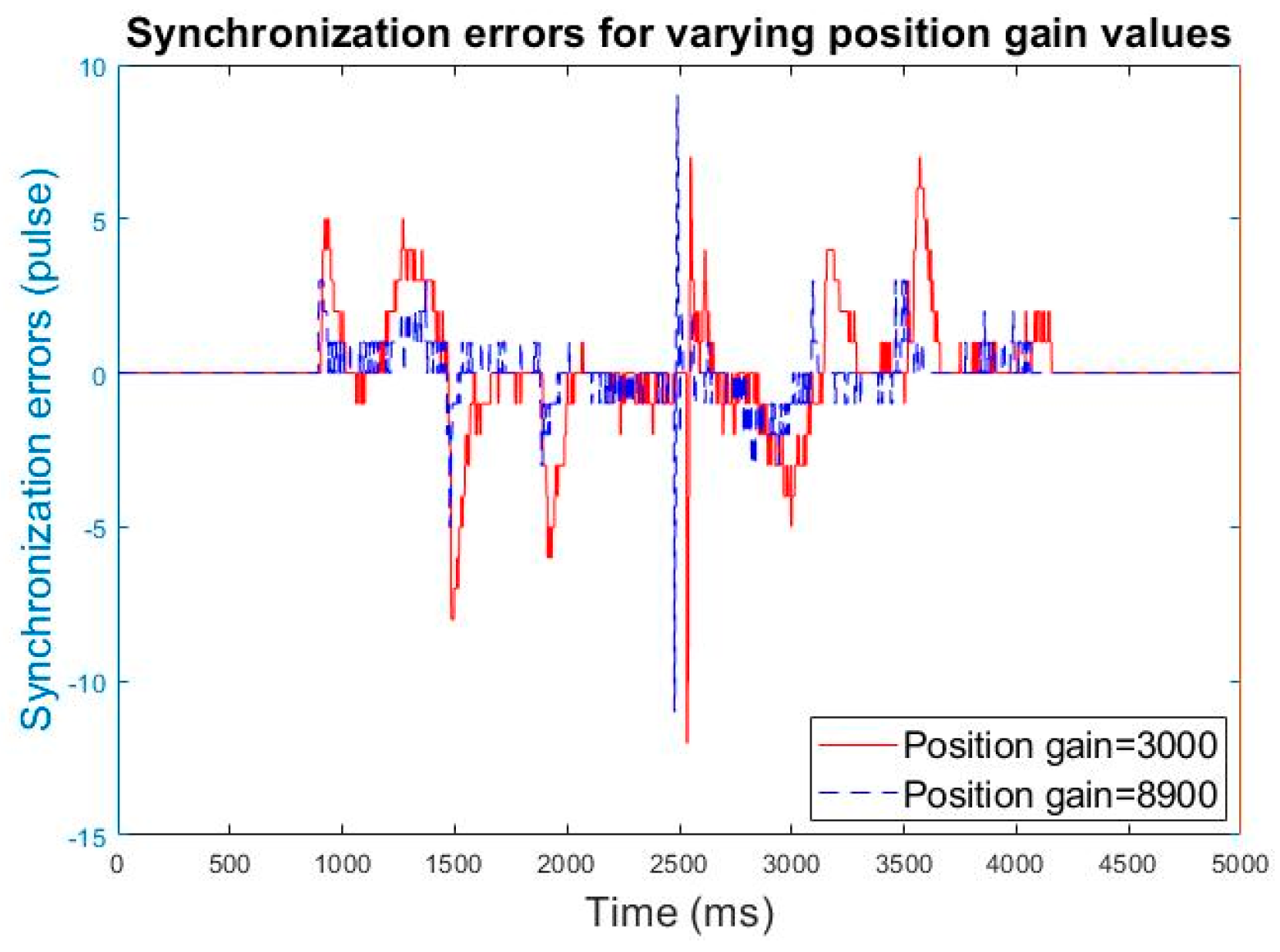
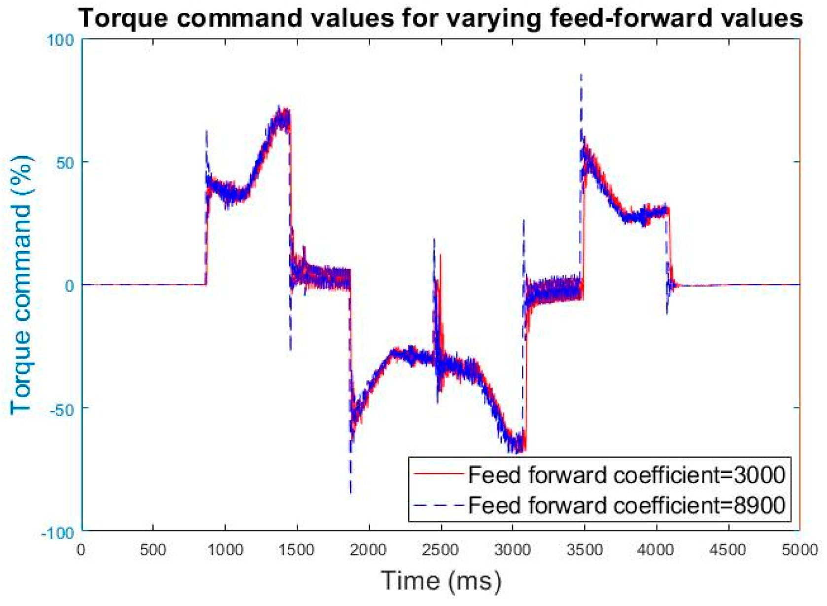
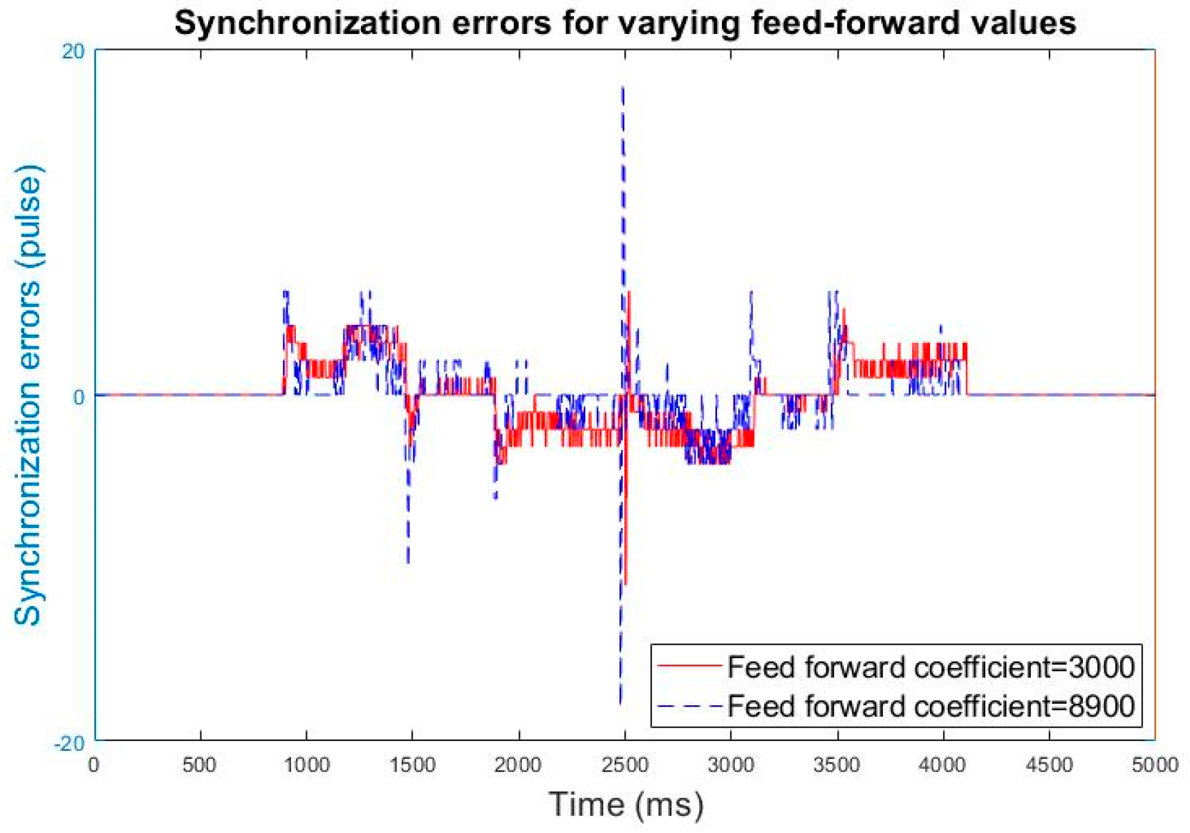
• Adjusting the position gain of the tapping axis and the feedforward coefficient can substantially decrease synchronization errors. Figure 7 and Figure 8 show how to position gain affects synchronization error and torque command. When position gain is significant, synchronization error is small, but current increases. Notably, the present value during air cut commissioning should not exceed 70–80%, and a reserve margin should be set to avoid overheating or overloading the motor during actual cutting. Air cut commissioning means dry run commissioning. Figure 9 and Figure 10 compare the effects of different feedforward coefficients on torque command.
• Adjusting the time required for motor excitation and stabilization can reduce errors at the start of rigid tapping.
• Reducing the z-axis following error, the synchronization error of rigid tapping can get better performance. After a synchronization error, reducing the z-axis following error and commissioning proportional gain, integral gain, and position gain can improve rigid tapping precision.

References

1. Lee, K.; Ibaraki, S.; Matsubara, A.; Kakino, Y.; Suzuki, Y.; Arai, S.; Braasch, J. A servo parameter tuning method for high-speed NC machine tools based on contouring error measurement. Laser Metrol. Mach. Perform. VI 2003, 44, 181–192. [Google Scholar]
2. Yeh, S.S.; Lee, J.I. Optimal tuning of control gains for rigid tapping processes using a learning automata methodology. In Proceedings of the IEEE Congress on Evolutionary Computation (CEC), Sendai, Japan, 25–28 May 2015; pp. 3248–3255. [Google Scholar]
3. Yeh, C.F.; Huang, W.S.; Kuo, C.H.; Hsu, P.L. Design and applications of the synchronized motion controller for tapping processes. In Proceedings of the 2012 XXth International Conference on Electrical Machines, Marseille, France, 2–5 September 2012; pp. 143–149. [Google Scholar]
4. Lu, J.; Zou, H.; Shen, L.; Zou, X. Application of adaptive fuzzy-pid control in servo spindle rigid tapping. Adv. Mater. Res. 2011, 301–303, 1477–1481. [Google Scholar] [CrossRef]
5. Sencer, B.; Ishizaki, K.; Shamoto, E. Cross coupling controller for accurate motion synchronization of dual servo systems. Int. J. Autom. Technol. 2013, 7, 514–522. [Google Scholar]
6. Biris, C.; Breaz, R.; Girjob, C.; Chicea, A. Researches regarding optimising the contouring precision of CNC laser cutting machines. Appl. Mech. Mater. 2014, 555, 580–585. [Google Scholar] [CrossRef]
7. Chen, S.L.; Pan, C.I.; Chou, C.Y. Reduction of synchronous errors in rigid tapping by iterative learning control. In Proceedings of the 2012 IEEE/ASME International Conference on Advanced Intelligent Mechatronics (AIM), Kaohsiung, Taiwan, 11–14 July 2012; pp. 467–471. [Google Scholar]
8. Andrearczyk, A.; Bagiński, P.; Klonowicz, P. Numerical and experimental investigations of a turbocharger with a compressor wheel made of additively manufactured plastic. Int. J. Mech. Sci. 2020, 178, 105613. [Google Scholar] [CrossRef]
9. Isaias Hernandez-Carrillo, I.; Wood, C.J.; Liu, H. Advanced materials for the impeller in an ORC radial microturbine. Energy Procedia 2017, 129, 1047–1054. [Google Scholar] [CrossRef]
10. Żywica, G.; Bagiński, P.; Andrearczyk, A. A new method of manufacturing a foil bearing using tools made by the rapid prototyping technology. CIRP J. Manuf. Sci. Technol. 2020, 31, 514–524. [Google Scholar] [CrossRef]
11. Bekker, A.C.M.; Verlinden, J.C. Life cycle assessment of wire + arc additive manufacturing compared to green sand casting and CNC milling in stainless steel. J. Clean. Prod. 2018, 177, 438–447. [Google Scholar] [CrossRef] [Green Version]
12. Andrearczyk, A.; Konieczny, B.; Sokołowski, J. Additively Manufactured Parts Made of a Polymer Material Used for the Experimental Verification of a Component of a High-Speed Machine with an Optimised Geometry-Preliminary Research. Polymers 2020, 13, 137. [Google Scholar] [CrossRef] [PubMed]
13. Yamazaki, T. Development of A Hybrid Multi-tasking Machine Tool: Integration of Additive Manufacturing Technology with CNC Machining. Procedia CIRP 2016, 42, 81–86. [Google Scholar] [CrossRef]
14. Chen, C.S.; Sun, Y.T.A. Intelligent Computer-aided Process Planning of Multi-axis CNC Tapping Machine. IEEE Access 2017, 5, 2913–2920. [Google Scholar] [CrossRef]
15. Ma, Y.C.; Wan, M.; Yang, Y.; Zhang, W.H. Dynamics of tapping process. Int. J. Mach. Tools Manuf. 2019, 140, 34–47. [Google Scholar] [CrossRef]
16. Ning, J.; Zhou, Y.; Fang, K.T. Discrepancy for uniform design of experiments with mixtures. J. Stat. Plan. Inference 2011, 141, 1487–1496. [Google Scholar] [CrossRef]
17. Wang, Y.; Fang, K.T. A note on uniform distribution and experimental design. Chin. Sci. Bull. 1981, 26, 485–489. [Google Scholar]
18. Fang, K.T. Uniform Design and Uniform Layout; Science Press: Beijing, China, 1994. [Google Scholar]
19. Tsao, H.; Lee, L. Uniform layout implement on MATLAB. Stat. Decis. 2008, 2008, 144–146. [Google Scholar]
20. Jebaseeli, E.A.E. Monitoring the thermal behavior of induction motor using regression technique. In Proceedings of the 2017 Innovations in Power and Advanced Computing Technologies (i-PACT), Vellore, India, 21–22 April 2017; pp. 1–4. [Google Scholar]
21. Yang, Y. Prediction and analysis of aero-material consumption based on multivariate linear regression model. In Proceedings of the 2018 IEEE 3rd International Conference on Cloud Computing and Big Data Analysis (ICCCBDA), Chengdu, China, 9–12 March 2018; pp. 628–632. [Google Scholar]
22. Pal, M.; Bharati, P. Applications of Regression Techniques; Springer: Singapore, 2019. [Google Scholar]
23. Olive, D. Linear Regression; Springer: New York, NY, USA, 2017. [Google Scholar]
24. Yang, P.-Y.; Chou, F.-I.; Tsai, J.-T.; Chou, J.-H. Adaptive-Uniform-Experimental-Design-Based Fractional-Order Particle Swarm Optimizer with Non-Linear Time-Varying Evolution. Appl. Sci. 2019, 9, 5537. [Google Scholar] [CrossRef] [Green Version]
25. Couceiro, M.; Ghamisi, P. Fractional Order Darwinian Particle Swarm Optimization; Springer: London, UK, 2016. [Google Scholar]
26. Guo, T.; Lan, J.L.; Li, Y.E.; Chen, S.W. Adaptive fractional-order Darwinian particle swarm optimization algorithm. J. Commun. 2014, 35, 130–140. [Google Scholar]
27. Solteiro Pires, E.J.; Tenreiro Machado, J.A.; Moura Oliveira, P.B.d. Fractional particle swarm optimization. In Mathematical Methods in Engineering; Fonseca, N.M., Tenreiro Machado, J.A., Eds.; Springer: London, UK, 2014; pp. 47–56. [Google Scholar]
28. Gao, Z.; Wei, J.; Liang, C.; Yan, M. Fractional-Order Particle Swarm Optimization. In Proceedings of the 26th Chinese Control and Decision Conference (CCDC), Changsha, China, 3 May–2 June 2014. [Google Scholar]
29. Hsu, C.C.; Yeh, S.S.; Lee, J.I. Effect analysis and optimal combination of cutting conditions on the cutting torque of tapping processes using Taguchi methods. In Proceedings of the 2016 IEEE International Conference on Automation Science and Engineering (CASE), Fort Worth, TX, USA, 21–25 August 2016; pp. 1215–1218. [Google Scholar]
30. Tsai, J.-T.; Chou, J.-H.; Liu, T.-K. Optimal design of digital IIR filters by using hybrid Taguchi genetic algorithm. IEEE Trans. Ind. Electron. 2006, 53, 867–879. [Google Scholar] [CrossRef]
31. Huang, W.-T.; Lee, T.-Y.; Chou, J.-H. Investigating Multiple Quality Objectives for Surface Roughness and Dimensional Accuracy of Carbon Steel Manufactured by Turn-Mill Multitasking Machining. In Proceedings of the 2018 IEEE International Conference on Advanced Manufacturing (ICAM), Yunlin, Taiwan, 16–18 November 2018; pp. 134–137. [Google Scholar]
32. Taguchi, G.; Chowdhury, S.; Taguchi, S. Robust Engineering; McGraw-Hill: New York, NY, USA, 2000. [Google Scholar]
33. Do, T.V.; Vu, N.C.; Nguyen, Q.M. Optimization of cooling conditions and cutting parameters during hard milling of AISI H13 steel by using Taguchi method. In Proceedings of the 2018 IEEE International Conference on Advanced Manufacturing (ICAM), Yunlin, Taiwan, 23–25 November 2018; pp. 396–398. [Google Scholar]
34. Weng, W.-C.; Yang, F.; Elsherbeni, A. Electromagnetics and Antenna Optimization using Taguchi’s Method. Synth. Lect. Comput. Electromagn. 2007, 2, 1–94. [Google Scholar] [CrossRef] [Green Version]
35. Luis-Ruiz, J.M.d.; Sedano-Cibrián, J.; Pereda-García, R.; Pérez-Álvarez, R.; Malagón-Picón, B. Optimization of Photogrammetric Flights with UAVs for the Metric Virtualization of Archaeological Sites. Application to Juliobriga (Cantabria, Spain). Appl. Sci. 2021, 11, 1204. [Google Scholar] [CrossRef]
36. Fernández, D.; Rodríguez-Prieto, A.; Camacho, A.M. Effect of Process Parameters and Definition of Favorable Conditions in Multi-Material Extrusion of Bimetallic AZ31B–Ti6Al4V Billets. Appl. Sci. 2020, 10, 8048. [Google Scholar] [CrossRef]
37. Hutchison, G.; Zahawi, B.; Giaouris, D.; Harmer, K.; Stedall, B. Parameter estimation of synchronous machines using particle swarm optimization. In Proceedings of the 2010 IEEE 11th International Conference on Probabilistic Methods Applied to Power Systems, Singapore, 14–17 June 2010; pp. 348–351. [Google Scholar]
38. Bhattacharyya, S.; Banerjee, P.; Dutta, P.; Majumdar, D. Handbook of Research on Advanced Hybrid Intelligent Techniques and Applications. Advances in Computational Intelligence and Robotics (ACIR) Book Series; IGI Global: Hershey, PA, USA, 2015. [Google Scholar]
39. Qin, B.; Yang, Y.; Liu, Y.; Wang, J. Improved particle swarm optimized fuzzy neural network based fault diagnosis for computer numerical control machine. In Proceedings of the 2015 IEEE International Conference on Mechatronics and Automation (ICMA), Beijing, China, 2–5 August 2015; pp. 1442–1447. [Google Scholar]
40. Zhu, G.-Y.; Zhang, W.-B. Drilling path optimization by the particle swarm optimization algorithm with global convergence characteristics. Int. J. Prod. Res. 2008, 46, 2299–2311. [Google Scholar] [CrossRef]
41. Chopard, B.; Tomassini, M. An Introduction to Metaheuristics for Optimization; Springer: Berlin, Germany, 2018. [Google Scholar]
42. Ali, M.M.; Kaelo, P. Improved Particle Swarm Algorithms for Global Optimization. Appl. Math. Comput. 2008, 196, 578–593. [Google Scholar] [CrossRef]
43. Chen, X.; Li, Y. On Convergence and Parameter Selection of an Improved Particle Swarm Optimization. Int. J. Control Autom. Syst. 2008, 6, 559–570. [Google Scholar]
44. Tsai, H.-C.; Tyan, Y.-Y.; Wu, Y.-W.; Lin, Y.H. Isolated Particle Swarm Optimization with Particle Migration and Global Best Adoption. Eng. Optim. 2012, 44, 1405–1424. [Google Scholar] [CrossRef]
45. Chen, W.-N.; Zhang, J.; Lin, Y.; Chen, N.; Zhan, Z.-H.; Chung, H.-S.-H.; Li, Y.; Shi, Y.-H. Particle Swarm Optimization with an Aging Leader and Challengers. IEEE Trans. Evol. Comput. 2013, 17, 241–258. [Google Scholar] [CrossRef]
46. Lynn, N.; Suganthan, P.N. Heterogeneous Comprehensive Learning Particle Swarm Optimization with Enhanced Exploration and Exploitation. Swarm Evol. Comput. 2015, 24, 11–24. [Google Scholar] [CrossRef]
47. Chatterjee, A.; Siarry, P. Nonlinear Inertia Weight Variation for Dynamic Adaptation in Particle Swarm Optimization. Comput. Oper. Res. 2006, 33, 859–871. [Google Scholar] [CrossRef]
48. Yang, X.; Yuan, J.; Yuan, J. A Modified Particle Swarm Optimizer with Dynamic Adaptation. Appl. Math. Comput. 2007, 189, 1205–1213. [Google Scholar] [CrossRef]
49. Ko, C.-N.; Chang, Y.-P.; Wu, C.-J. An Orthogonal-Array-based Particle Swarm Optimizer with Nonlinear Time-Varying Evolution. Appl. Math. Comput. 2007, 191, 272–279. [Google Scholar] [CrossRef]
50. Tsai, J.-T.; Chou, P.-Y.; Chou, J.-H. Color Filter Polishing Optimization Using ANFIS with Sliding-Level Particle Swarm Optimizer. IEEE Trans. Syst. Man Cybern. Syst. 2020, 50, 1193–1207. [Google Scholar] [CrossRef]
51. Xin, B.; Chen, J. A Survey and Taxonomy on Hybrid Algorithms based on Particle Swarm Optimization and Differential Evolution. J. Syst. Sci. Math. Sci. 2011, 31, 1130–1150. [Google Scholar]
52. Noel, M.M. A New Gradient Based Particle Swarm Optimization Algorithm for Accurate Computation of Global Minimum. Appl. Soft Comput. 2012, 12, 353–359. [Google Scholar] [CrossRef]
53. Sun, Y.; Zhang, L.; Gu, X. A Hybrid Co-Evolutionary Cultural Algorithm based on Particle Swarm Optimization for Solving Global Optimization Problems. Neurocomputing 2012, 98, 76–89. [Google Scholar] [CrossRef]
54. B-65264EN. Fanuc Servo Tuning Procedure Manual; Fanuc Corporation: Yamanashi, Japan, 2005. [Google Scholar]
55. B-65280EN/07. Fanuc AC Spindle Motor Alpha-i series Parameter Manual; Fanuc Corporation: Yamanashi, Japan, 2008. [Google Scholar]
56. B-65270EN/07. Fanuc AC Servo Motor Alpha-i series Parameter Manual; Fanuc Corporation: Yamanashi, Japan, 2007. [Google Scholar]
57. B-63950EN. Fanuc Series 30i/300i/300is-MODEL-A Parameter Manual; Fanuc Corporation: Yamanashi, Japan, 2004. [Google Scholar]
Figure 1. Measurements used for the analysis of screw teeth.
Applsci 11 03441 g001
Figure 2. Tapping center machine (YCM NDV102A) used for the experiments in this study.
Applsci 11 03441 g002
Figure 3. Diagram of rigid tapping path relationship.
Applsci 11 03441 g003
Figure 4. Flowchart of the experimental procedure.
Applsci 11 03441 g004
Figure 5. Response table from Table 13. (a) Proportional gain of velocity loop for spindle in servo mode; (b) Delay time for motor excitation; (c) Integral gain of velocity loop for spindle in servo mode; (d) Advanced feedforward; (e) Position gain of servo axis for rigid tap.
Applsci 11 03441 g005
Figure 6. Synchronization error waveforms in rigid tapping before (a) and after commissioning (b).
Applsci 11 03441 g006
Figure 7. Torque command values for varying position gain values in rigid tapping.
Applsci 11 03441 g007
Figure 8. Synchronization errors for varying position gain values in rigid tapping.
Applsci 11 03441 g008
Figure 9. Torque command values for varying feedforward coefficients.
Applsci 11 03441 g009
Figure 10. Synchronization errors for varying advanced feedforward coefficients.
Applsci 11 03441 g010