Search Patterns Based on Trajectories Extracted from the Response of Second-Order Systems

Abstract

Recently, several new metaheuristic schemes have been introduced in the literature. Although all these approaches consider very different phenomena as metaphors, the search patterns used to explore the search space are very similar. On the other hand, second-order systems are models that present different temporal behaviors depending on the value of their parameters. Such temporal behaviors can be conceived as search patterns with multiple behaviors and simple configurations. In this paper, a set of new search patterns are introduced to explore the search space efficiently. They emulate the response of a second-order system. The proposed set of search patterns have been integrated as a complete search strategy, called Second-Order Algorithm (SOA), to obtain the global solution of complex optimization problems. To analyze the performance of the proposed scheme, it has been compared in a set of representative optimization problems, including multimodal, unimodal, and hybrid benchmark formulations. Numerical results demonstrate that the proposed SOA method exhibits remarkable performance in terms of accuracy and high convergence rates.

1. Introduction

Metaheuristic algorithms refer to generic optimization schemes that emulate the operation of different natural or social processes. In metaheuristic approaches, the optimization strategy is performed by a set of search agents. Each agent maintains a possible solution to the optimization problem, and is initially produced by considering a random feasible solution. An objective function determines the quality of the solution of each agent. By using the values of the objective function, at each iteration, the position of the search agents is modified, employing a set of search patterns that regulate their movements within the search space. Such search patterns are abstract models inspired by natural or social processes [1]. These steps are repeated until a stop criterion is reached. Metaheuristic schemes have confirmed their supremacy in diverse real-world applications in circumstances where classical methods cannot be adopted.

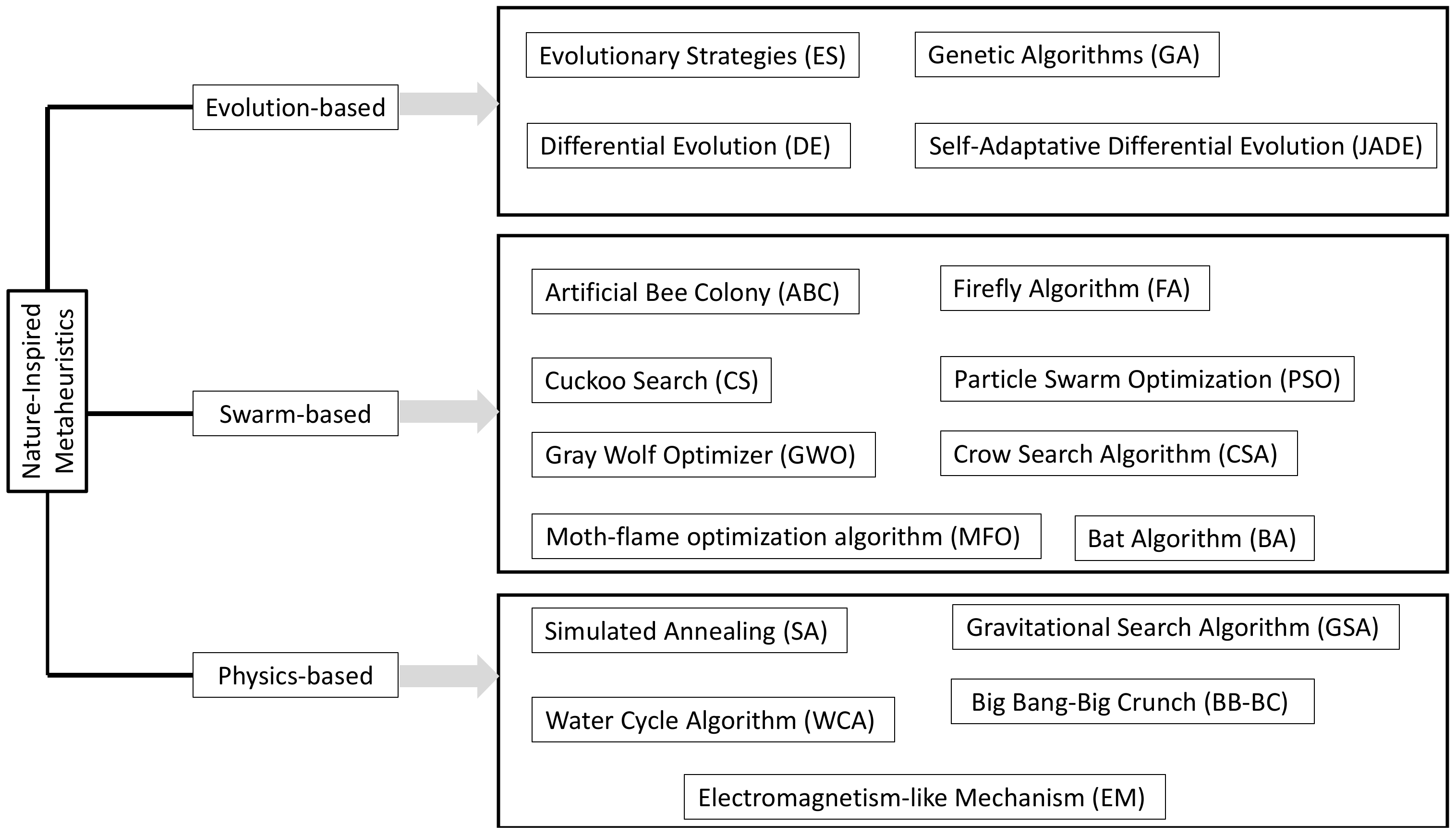
Essentially, a clear classification of metaheuristic methods does not exist. Despite this, several categories have been proposed that considered different criteria, such as a source of inspiration, type of operators or cooperation among the agents. In relation to inspiration, nature-inspired metaheuristic algorithms are classified into three categories: Evolution-based, swarm-based, and physics-based. Evolution-based approaches correspond to the most consolidate search strategies that use evolution elements as operators to produce search patterns. Consequently, operations, such as reproduction, mutation, recombination, and selection are used to generate search patterns during their operations. The most representative examples of evolution-based techniques, include Evolutionary Strategies (ES) [2,3,4], Genetic Algorithms (GA) [5], Differential Evolution (DE) [6] and Self-Adaptative Differential Evolution (JADE) [7]. Swarm-inspired techniques use behavioral schemes extracted from the collaborative interaction of different animals or species of insects to produce a search strategy. Recently, a high number of swarm-based approaches have been published in the literature. Among the most popular swarm-inspired approaches, include the Crow Search Algorithm (CSA) [8], Artificial Bee Colony (ABC) [9], Particle Swarm Optimization (PSO) algorithm [10,11,12], Firefly Algorithm (FA) [13,14], Cuckoo Search (CS) [15], Bat Algorithm (BA) [16], Gray Wolf Optimizer (GWO) [17], Moth-flame optimization algorithm (MFO) [18] to name a few. Metaheuristic algorithms that consider the physics-based scheme use simplified physical models to produce search patterns for their agents. Some examples of the most representative physics-based techniques involve the States of Matter Search (SMS) [19,20], the Simulated Annealing (SA) algorithm [21,22,23], the Gravitational Search Algorithm (GSA) [24], the Water Cycle Algorithm (WCA) [25], the Big Bang-Big Crunch (BB-BC) [26] and Electromagnetism-like Mechanism (EM) [27]. Figure 1 visually exhibits the taxonomy of the metaheuristic classification. Although all these approaches consider very different phenomena as metaphors, the search patterns used to explore the search space are exclusively based on spiral elements or attraction models [10,11,12,13,14,15,16,17,28]. Under such conditions, the design of many metaheuristic methods refers to configuring a recycled search pattern that has been demonstrated to be successful in previous approaches for generating new optimization schemes through a marginal modification.

On the other hand, the order of a differential equation refers to the highest degree of derivative considered in the model. Therefore, a model whose input-output formulation is a second-order differential equation is known as a second-order system [29]. One of the main elements that make a second-order model important is its ability to present very different behaviors, depending on the configuration of its parameters. Through its different behaviors, such as oscillatory, underdamped, or overdamped, a second-order system can exhibit distinct temporal responses [30]. Such behaviors can be observed as search trajectories under the perspective of metaheuristic schemes. Therefore, with second-order systems, it is possible to produce oscillatory movements within a certain region or build complex search patterns around different points or sections of the search space.

In this paper, a set of new search patterns are introduced to explore the search space efficiently. They emulate the response of a second-order system. The proposed set of search patterns have been integrated as a complete search strategy, called Second-Order Algorithm (SOA), to obtain the global solution of complex optimization problems. To analyze the performance of the proposed scheme, it has been compared in a set of representative optimization problems, including multimodal, unimodal, and hybrid benchmark formulations. The competitive results demonstrate the promising results of the proposed search patterns.

The main contributions of this research can be stated as follows:

• A new physics-based optimization algorithm, namely SOA, is introduced. It uses search patterns obtained from the response of second-order systems.
• New search patterns are proposed as an alternative to those known in the literature.
• The statistical significance, convergence speed and exploitation-exploration ratio of SOA are evaluated against other popular metaheuristic algorithms.
• SOA outperforms other competitor algorithms on two sets of optimization problems.

The remainder of this paper is structured as follows: A brief introduction of the second-order systems is given in Section 2; in Section 3, the most important search patterns in metaheuristic methods are discussed; in Section 4, the proposed search patterns are defined; in Section 5, the measurement of exploration-exploitation is described; in Section 6, the proposed scheme is introduced; Section 7 presents the numerical results; in Section 8, the main characteristics of the proposed approach are discussed; in Section 9, finally, the conclusions are drawn.

2. Second-Order Systems

A model whose input $R\left(s\right)$-output $C\left(s\right)$ formulation is a second-order closed-loop transfer function is known as a second-order system. One of the main elements that make a second-order model important is its ability to present very different behaviors depending on the configuration of its parameters. A generic second-order model can be formulated under the following expression [29],

$$\frac{C\left(s\right)}{R\left(s\right)}=\frac{{\omega }_n^2}{s^2+2\zeta {\omega }_{n}s+{\omega }_n^2},$$

(1)

where ζ and ω_n represent the damping ratio and ω_n the natural frequency, respectively, while s symbolizes the Laplace domain.

The dynamic behavior of a system is evaluated in terms of the temporal response obtained through a unitary step signal as input $R\left(s\right)$. The dynamic behavior is defined as the way in which the system reacts, trying to reach the value of one as time evolves. The dynamic behavior of the second-order system is described in terms of $\zeta$ and ${\omega }_n$ [30]. Assuming such parameters, the second-order system presents three different behaviors: Underdamped ($0<\zeta <1)$, critically damped ($\zeta =1)$, and overdamped ($\zeta >1)$.

2.1. Underdamped Behavior ($0<\zeta <1)$

In this behavior, the poles (roots of the denominator) of Equation (1) are complex conjugated and located in the left-half of the $s$ plane. Under such conditions, the system underdamped response $C_U\left(s\right)$ in the Laplace domain can be characterized as follows:

$$C_U\left(s\right)=\frac{{\omega }_n^2}{s{\left(s+\zeta {\omega }_n\right)}^2+{\omega }_n^2\left(1-{\zeta }^2\right)}.$$

(2)

Applying partial fraction operations and the inverse Laplace transform, it is obtained the temporal response that describe the underdamped behavior $c_U\left(t\right)$ as it is indicated in Equation (3):

$$c_U\left(t\right)=1-\frac{e^{-\zeta {\omega }_{n}t}}{\sqrt{1-{\zeta }^2}}\sin \left({\omega }_n\sqrt{1-{\zeta }^2}+{\tan }^{-1}\left(\frac{\sqrt{1-{\zeta }^2}}{\zeta }\right)\right).$$

(3)

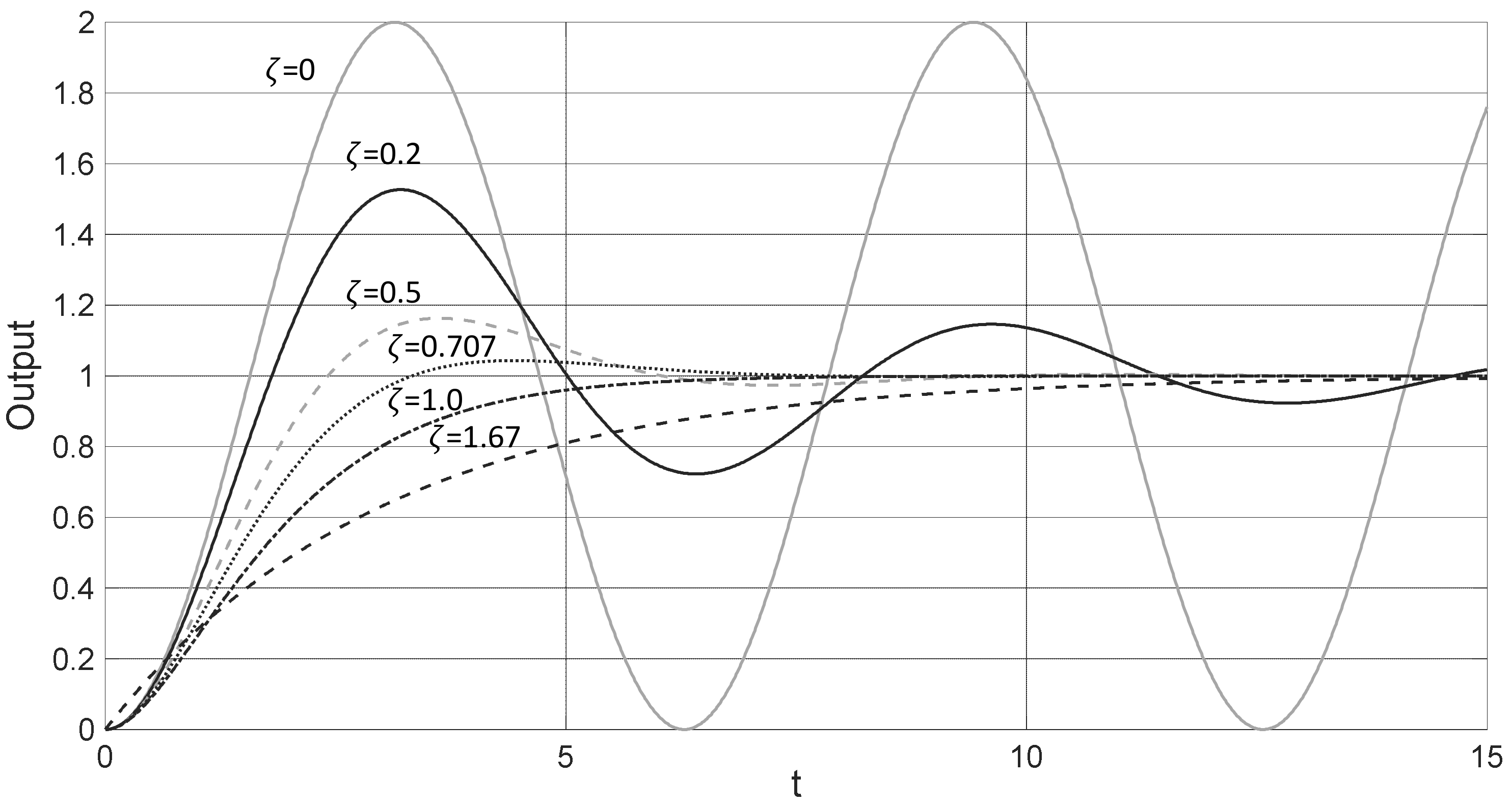
If $\zeta =0$, a special case is presented in which the temporal system response is oscillatory. The output of these behaviors is visualized in Figure 2 for the cases of $\zeta =0$, $\zeta =0.2$, $\zeta =0.5$ and $\zeta =0.707$. Under the underdamped behavior, the system response starts with high acceleration. Therefore, the response produces an overshoot that surpasses the value of one. The size of the overshoot inversely depends on the value of $\zeta$.

2.2. Critically Damped Behavior ($\zeta =1)$

Under this behavior, the two poles of the transfer function of Equation (1) present a real number and maintain the same value. Therefore, the response of the critically damped behavior $C_C\left(s\right)$ in the Laplace domain can be described as follows:

$$C_C\left(s\right)=\frac{{\omega }_n^2}{s{\left(s+{\omega }_n\right)}^2}.$$

(4)

Considering the inverse Laplace transform of Equation (4), the temporal response of the critically damped behavior $c_C\left(t\right)$ is determined under the following model:

$$c_C\left(t\right)=1-e^{-{\omega }_{n}t}\left(1+{\omega }_{n}t\right).$$

(5)

Under the critically damped behavior, the system response presents a temporal pattern similar to a first-order system. It reaches the objective value of one without experimenting with an overshoot. The output of the critically damped behavior is visualized in Figure 2.

2.3. Overdamped Behavior ($\zeta >1)$

In the overdamped case, the two poles of a transfer function of Equation (1) have real numbers but with different values. Its response $C_O\left(s\right)$ in the Laplace domain is modeled under the following formulation:

$$C_O\left(s\right)=\frac{{\omega }_n^2}{s\left(s+\zeta {\omega }_n+{\omega }_n\sqrt{{\zeta }^2-1}\right)\left(s+\zeta {\omega }_n-{\omega }_n\sqrt{{\zeta }^2-1}\right)}.$$

(6)

After applying the inverse Laplace transform, it is obtained the temporal response of the overdamped behavior $c_O\left(t\right)$ defined as follows:

$$c_O\left(t\right)=1+e^{-\left(\zeta -\sqrt{{\zeta }^2-1}\right){\omega }_{n}t}.$$

(7)

Under the Overdamped behavior, the system slowly reacts until reaching the value of one. The deceleration of the response depends on the value of $\zeta$. The greater the value of $\zeta$, the slower the response will be. The output of this behavior is visualized in Figure 2 for the case of $\zeta =1.67$.

3. Search Patterns in Metaheuristics

The generation of efficient search patterns for the correct exploration of a fitness landscape could be complicated, particularly in the presence of ruggedness and multiple local optima. Recently, several new metaheuristic schemes have been introduced in the literature. Although all these approaches consider very different phenomena as metaphors, the search patterns, used to explore the search space, are very similar. A search pattern is a set of movements produced by a rule or model in order to examine promising solutions from the search space.

Exploration and exploitation correspond to the most important characteristics of a search pattern. Exploration refers to the ability of a search pattern to examine a set of solutions spread in distinct areas of the search space. On the other hand, exploitation represents the capacity of a search pattern to improve the accuracy of the existent solutions through a local examination. The combination of both mechanisms in a search pattern is crucial for attaining success when solving a particular optimization problem.

To solve the optimization formulation, from a metaheuristic point of view, a population of $P^k$ $\left(\left\{x_1^k,\dots ,x_N^k\right\}\right)$ of $N$ candidate solutions (individuals) evolve from an initial point ($k$ = 1) to a $Maxgen$ number of generations ($k=Maxgen$). In the population, each individual $x_i^k$ $\left(i\in \left[1,\dots ,N\right]\right)$ corresponds to a $d$-dimensional element $\left\{x_{i,1}^k,\dots ,x_{i,d}^k\right\},$ which symbolizes the decision variables involved by the optimization problem. At each generation, search patterns are applied over the individuals of the population $P^k$ to produce the new population $P^{k+1}$. The quality of each individual $x_i^k$ is evaluated in terms of its solution regarding the objective function $J\left(x_i^k\right)$ whose result represents the fitness value of $x_i^k$. As the metaheuristic method evolves, the best current individual $b$ $\left\{b_1,\dots ,b_d\right\}$ is maintained since $b$ represents the best available solution seen so-far.

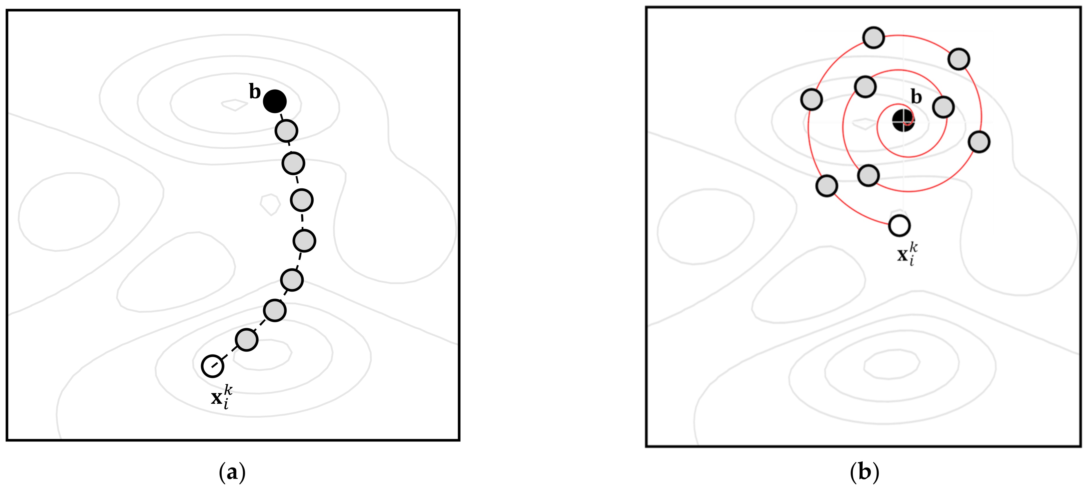
In general, a search pattern is applied to each individual $x_i^k$ using the best element $b$ as a reference. Then, following a particular model, a set of movements are produced to modify the position of $x_i^k$ until the location of $b$ has been reached. The idea behind this mechanism is to examine solutions in the trajectory from $x_i^k$ to $b$ with the objective to find a better solution than the current $b$. Search patterns differ in the model employed to produce the trajectories $x_i^k$ from to $b$.

Two of the most popular search models are attraction and spiral trajectories. The attraction model generates attraction movements from $x_i^k$ to $b$. The attraction model is used extensively by several metaheuristic methods such as PSO [10,11,12], FA [13,14], CS [15], BA [16], GSA [24], EM [27] and DE [6]. On the other hand, the spiral model produces a spiral trajectory that encircles the best element $b$. The spiral model is employed by the recently published WOA and GWO schemes. Trajectories produced by the attraction, and spiral models are visualized in Figure 3a,b, respectively.

4. Proposed Search Patterns

In this paper, a set of new search patterns are introduced to explore the search space efficiently. They emulate the response of a second-order system. The proposed set of search patterns have been integrated as a complete search strategy to obtain the global solution of complex optimization problems. Since the proposed scheme is based on the response of the second-order systems, it can be considered as a physics-based algorithm. In our approach, the temporal response of second-order system is used to generate the trajectory from the position of $x_i^k=\left\{x_{i,1}^k,\dots ,x_{i,d}^k\right\}$ to the location of $b=\left\{b_1,\dots ,b_d\right\}$. 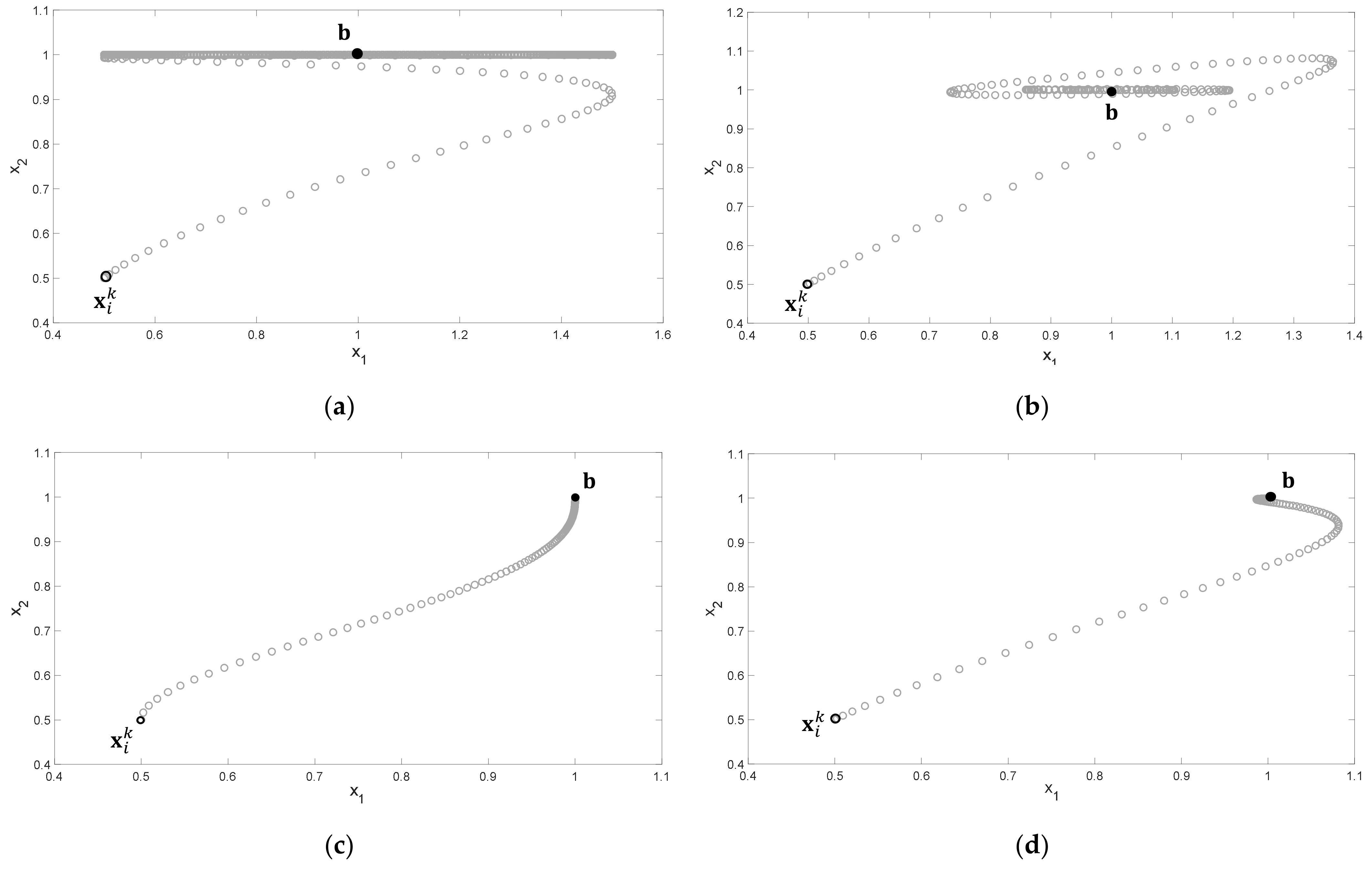With the use of such models, it is possible to produce more complex trajectories that allow a better examination of the search space. Under such conditions, we consider the three different responses of a second-order system to produce three distinct search patterns. They are the underdamped, critically damped and overdamped modeled by the expressions Equations (8)–(10), respectively:

$$x_{i,j}^k=\left(1-\frac{e^{-\zeta {\omega }_{n}k}}{\sqrt{1-{\zeta }^2}}\sin \left({\omega }_n\sqrt{1-{\zeta }^2}+{\tan }^{-1}\left(\frac{\sqrt{1-{\zeta }^2}}{\zeta }\right)\right)\right)\left(b_j-x_{i,j}^k\right);$$

(8)

$$x_{i,j}^k=\left(1-e^{-{\omega }_{n}k}\left(1+{\omega }_{n}k\right)\right)\left(b_j-x_{i,j}^k\right);$$

(9)

$$x_{i,j}^k=\left(1+e^{-\left(\zeta -\sqrt{{\zeta }^2-1}\right){\omega }_{n}k}\right)\left(b_j-x_{i,j}^k\right);$$

(10)

where $i$ ($\in \left[1,N\right]$) corresponds to the search agent while $j$ ($\in \left[1,d\right]$) symbolizes the decision variable or dimension. Since the behavior of each search pattern depends on the value of $\zeta$, it is easy to combine elements to produce interesting trajectories. Figure 4 presents some examples of trajectories produced by using different values for $\zeta$. In the Figure, it is assumed a two-dimensional case ($d=2$) where the initial position of the search agent $x_i^k$ is $\left(0.5,0.5\right)$ and the final location or the best location $\left(1,1\right)$. Figure 4a presents the case of $x_{i,1}^k\leftarrow \zeta =0$ and $x_{i,2}^k\leftarrow \zeta =1$. Figure 4b presents the case of $x_{i,1}^k\leftarrow \zeta =0.1$ and $x_{i,2}^k\leftarrow \zeta =0.5$. Figure 4c presents the case of $x_{i,1}^k\leftarrow \zeta =1$ and $x_{i,2}^k\leftarrow \zeta =1.67$. Finally, Figure 4d presents the case of $x_{i,1}^k\leftarrow \zeta =0.5$ and $x_{i,2}^k\leftarrow \zeta =1$. From the figures, it is clear that the second-order responses allow producing several complex trajectories, which include most of the other search patterns known in the literature. In all cases (a)–(d), the value of ${\omega }_n$ has been set to 1.

5. Balance of Exploration and Exploitation

Metaheuristic methods employ a set of search agents to examine the search space with the objective to identify a satisfactory solution for an optimization formulation. In metaheuristic schemes, search agents that present the best fitness values tend to regulate the search process, producing an attraction towards them. Under such conditions, as the optimization process evolves, the distance among individuals diminishes while the effect of exploitation is highlighted. On the other hand, when the distance among individuals increases, the characteristics of the exploration process are more evident.

To compute the relative distance among individuals (increase and decrease), a diversity indicator known as the dimension-wise diversity index [31] is used. Under this approach, the diversity is formulated as follows,

$$\begin{gathered} Di{v}_j= \frac{1}{N}{\displaystyle \sum }_{i=1}^N\left|median\left(x^j\right)- x_{i,j}\right| \\ Div=\frac{1}{d} {\displaystyle \sum }_{j=1}^{d}Di{v}_j \end{gathered}$$

(11)

where $median\left(x^j\right)$ symbolizes the median of dimension $j$ of all search agents. $x_{i,j}$ represents the variable decision $j$ of the individual $i$. $N$ is the number of individuals in the population $P^k$ while $d$ corresponds to the number of dimensions of the optimization formulation. The diversity $Di{v}_j$ (of the $j$-th dimension) evaluates the relative distance between the variable $j$ of each individual and its median value. The complete diversity $Div$ (of the entire population) corresponds to the averaged diversity in each dimension. Both elements $Di{v}_j$ and $Div$ are calculated in every iteration.

Having evaluated the diversity values, the level of exploration and exploitation can be computed as the percentage of the time that a search strategy invests exploring or exploiting in terms of its diversity values. These percentages are calculated in each iteration by means of the following models,

$$\begin{gathered} XPL\%= \left(\frac{Div}{Di{v}_{max}}\right)\times 100 \\ XPT\%= \left(\frac{\left|Div-Di{v}_{max}\right|}{Di{v}_{max}}\right)\times 100 \end{gathered}$$

(12)

where $Di{v}_{max}$ symbolizes the maximum diversity value obtained during the optimization process. The percentage of exploration $XPL\%$ corresponds to the size of exploration as the rate between $Div$ and $Di{v}_{max}$. On the other hand, the percentage of exploitation $XPT\%$ symbolizes the level of exploitation. $XPT\%$ is computed as the complemental percentage to $XPL\%$ since the difference between $Di{v}_{max}$ and $Div$ is generated because of the concentration of individuals.

6. Proposed Metaheuristic Algorithm

The set of search patterns based on the second-order systems have been integrated as a complete search strategy to obtain the global solution of complex optimization problems. In this section, the complete metaheuristic method, called Second-Order Algorithm (SOA), is completely described.

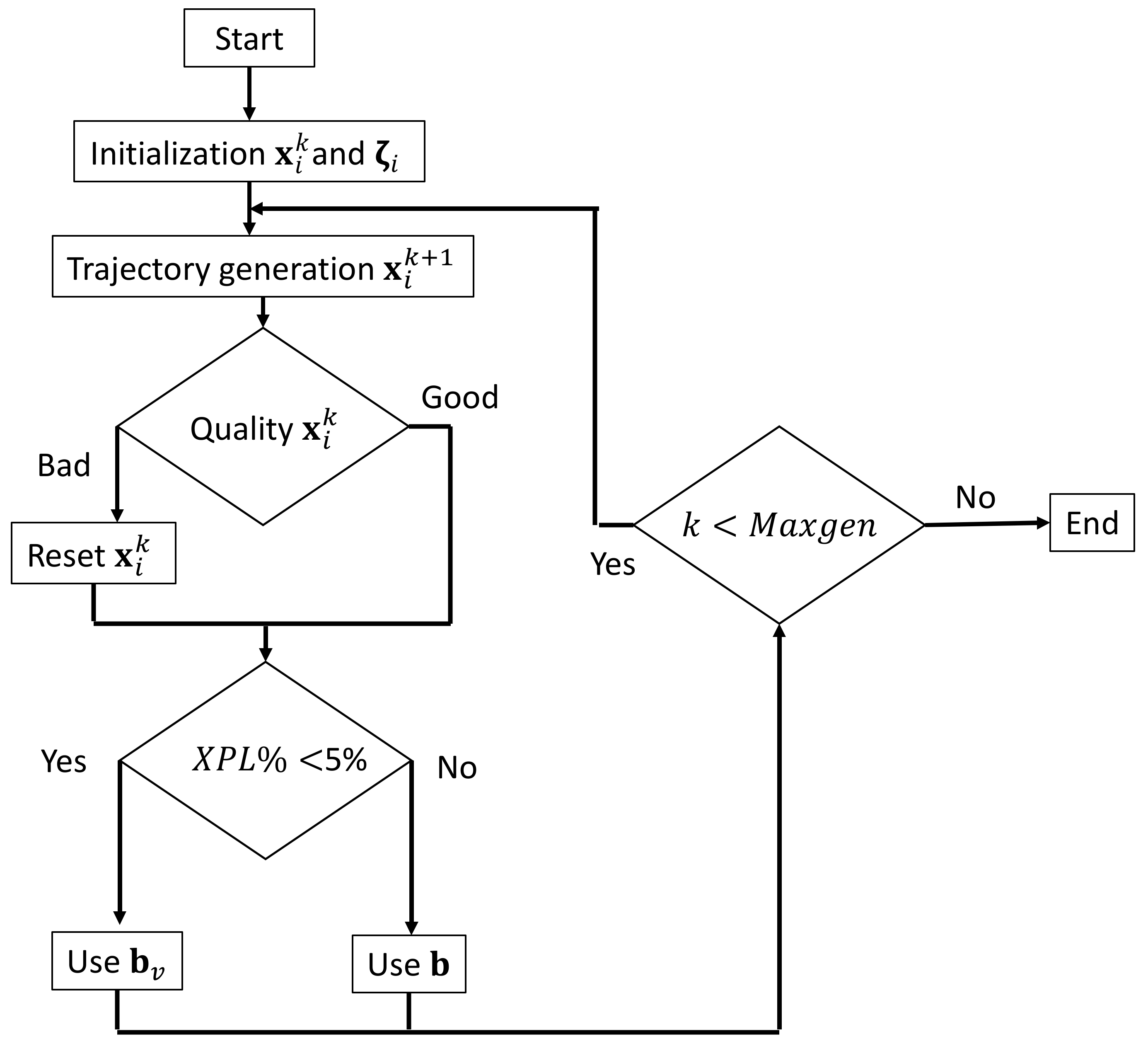
The scheme considers four different stages: (A) Initialization, (B) trajectory generation, (C) reset of bad elements, and (D) avoid premature convergence mechanism. The steps (B)–(D) are sequentially executed until a stop criterion has been reached. Figure 5 shows the flowchart of the complete metaheuristic method.

6.1. Initialization

In the first iteration $k=0$, a population $P^0$ of $N$ agents $\left\{x_1^0,\dots ,x_N^0\right\}$ is randomly produced considering to the following equation,

$$\begin{gathered} x_{i,j}^0=rand·\left(b_j^{high}-b_j^{low}\right)+b_j^{low} \\ i=1, 2, \dots , N; j=1,\dots ,d \end{gathered}$$

(13)

where $b_j^{high}$ and $b_j^{low}$ are the limits of the $j$ decision variable and $rand$ is a uniformly distributed random number between [0,1].

To each individual $x_i$ from the population, it is assigned a vector ${\mathsf{\zeta }}_i=\left\{{\zeta }_{i,1}, \dots ,{\zeta }_{i,d}\right\}$ whose elements ${\zeta }_{i,j}$ determine the trajectory behavior of each $j$-th dimension. Initially, each element ${\zeta }_{i,j}$ is set to a random value between [0,2]. Under this interval, all the second-order behavior are possible: Underdamped ($0<\zeta <1)$, critically damped ($\zeta =1)$, and overdamped ($\zeta >1)$.

6.2. Trajectory Generation

Once the population has been initialized, it is obtained the best element of the population $b$. Then, the new position $x_i^{k+1}$ of each agent $x_i^k$ is computed as a trajectory generated by a second-order system. Once all new positions in the population $P^k$ are determined, it is also defined the best element $b$.

6.3. Reset of Bad Elements

To each agent $x_i^k$ is allowed to move in its own trajectory for ten iterations. After ten iterations, if the search agent $x_i^k$ maintains the worst performance in terms of the fitness function, it is reinitialized in both position and in its vector ${\mathsf{\zeta }}_i$. Under such conditions, the search agent will be in another position and with the ability to perform another kind of trajectory behavior.

6.4. Avoid Premature Convergence Mechanism

If the percentage of exploration $XPL\%$ is less than 5%, the best value $b$ is replaced by the best virtual value $b_v$. The element $b_v$ is computed as the averaged value of the best five individuals of the population. The idea behind this mechanism is to identify a new position to generate different trajectories that avoid that the search process gets trapped in a local optimum.

7. Experimental Results

To evaluate the results of the proposed SOA algorithm, a set of experiments has been conducted. Such results have been compared to those produced by the Artificial Bee Colony (ABC) [9], the Covariance matrix adaptation evolution strategy (CMAES) [4], the Crow Search Algorithm (CSA) [8], the Differential Evolution (DE) [6], the Moth-flame optimization algorithm (MFO) [18] and the Particle Swarm Optimization (PSO) [10], which are considered the most popular metaheuristic schemes in many optimization studies [32].

For the comparison, all methods have been set according to their reported guidelines. Such configurations are described as follows:

• ABC: Onlooker Bees = 50, acceleration coefficient = 1 [9].
• DE: crossover probability = 0.2, Betha = 1 [6].
• CMAES: Lambda = 50, father number = 25, sigma = 60, csigma = 0.32586, dsigma = 1.32586 [4].
• CSA: Flock = 50, awareness probability = 0.1, flight length = 2 [8].
• MFO: search agents = 50, “a” linearly decreases from 2 to 0 [18].
• SOA: the experimental results give the best algorithm performance with the next parameter set par1 = 0.7, par2 = 0.3 and par3 = 0.05.

In our analysis, the population size N has been set to 50 search agents. The maximum iteration number $\left(Maxgen\right)$ for all functions has been set to 1000. This stop criterion has been decided to keep compatibility with similar works published in the literature [33,34]. To evaluate the results, three different indicators are considered: The Average Best-so-far (AB) solution, the Median Best-so-far (MB) solution and the Standard Deviation (SD) of the best-so-far solutions. In the analysis, each optimization problem is solved using every algorithm 30 times. From this operation, 30 results are produced. From all these values, the mean value of all best-found solutions represents the Average Best-so-far (AB) solution. Likewise, the median of all 30 results is computed to generate MB and the standard deviation of the 30 data is estimated to obtain SD of the best-so-far solutions. Indicators AB and MB correspond to the accuracy of the solutions, while SD their dispersion, and thus, the robustness of the algorithm.

The experimental section is divided into five sub-sections. In the first Section 7.1, the performance of SOA is evaluated with regard to multimodal functions. In the second Section 7.2, the results of the OTSA method in comparison with other similar approaches are analyzed in terms of unimodal functions. In the third Section 7.3, a comparative study among the algorithms examining hybrid functions is accomplished. In the fourth Section 7.4, the ability of all algorithms to converge is analyzed. Finally, in the fifth Section 7.5, the performance of the SOA method to solve the CEC 2017 set of functions is also analyzed.

7.1. Multimodal Functions

In this sub-section, the SOA approach is evaluated considering 12 unimodal functions ($f_1\left(x\right)–f_{12}\left(x\right))$ reported in

Table A1. List of Benchmark Functions.

	Name	Function	S	Dim	Minimum
$f_1\left(\mathrm{x}\right)$	Levy	$si{n}^2\left(\pi {\omega }_1\right)+{\displaystyle {\displaystyle \sum }_{i=1}^{d-1}}{\left({\omega }_i-1\right)}^2\left[1+10si{n}^2\left(\pi {\omega }_i+1\right)+{\left({\omega }_d-1\right)}^2\left[1+si{n}^2\left(2\pi {\omega }_d\right)\right]\right]$	${\left[-10, 10\right]}^n$	30	$f\left(x^{*}\right)=0;$ $x^{*}=\left(1,\dots , 1\right)$
$f_2\left(\mathrm{x}\right)$	Mishra 1	${\left(1+x_n\right)}^{x_n}; x_n=n-{{\displaystyle \sum }}_{i=1}^{n-1}{x}_i$	${\left[0, 1\right]}^n$	30	$f\left(x^{*}\right)=2;$ $x^{*}=\left(1,\dots , 1\right)$
$f_3\left(\mathrm{x}\right)$	Mishra 2	${\left(1+x_n\right)}^{x_n}; x_n=n-{{\displaystyle \sum }}_{i=1}^{n-1}\frac{\left(x_i+x_{i+1}\right)}{2}$	${\left[0, 1\right]}^n$	30	$f\left(x^{*}\right)=2;$ $x^{*}=\left(1,\dots , 1\right)$
$f_4\left(\mathrm{x}\right)$	Mishra 11	$\left[\frac{1}{n}{\displaystyle {\displaystyle \sum }_{i=1}^n}\left|x_i\right|-{\left({\displaystyle {\displaystyle \prod }_{i=1}^n}\left|x_i\right|\right)}^{\frac{1}{n}}\right]{ }^2$	${\left[-10, 10\right]}^n$	30	$f\left(x^{*}\right)=0;$ $x^{*}=\left(0,\dots , 0\right)$
$f_5\left(\mathrm{x}\right)$	Penalty 1	$\frac{\pi }{30}\left\{\begin{array}{c}10{\sin }^2\left(\pi y_1\right)\\ +{{\displaystyle \sum }}_{i=1}^{n-1}{\left(y_i-1\right)}^2\left[1+10{\sin }^2\left(\pi y_i+1\right)\right]\\ +{\left(y_n-1\right)}^2\end{array}\right\}+{{\displaystyle \sum }}_{i=1}^{n}u\left(x_i, 10, 100, 4\right);$ $y_i=1+\frac{x_i+1}{4};$ $u\left(x_i, a, k, m\right)=\left\{\begin{array}{c}k{\left(x_i-a\right)}^m, x_i>a\\ 0, -a\le x_i\le a\\ k{\left(-x_i-a\right)}^m, x_i<-a\end{array}\right.$	${\left[-50, 50\right]}^n$	30	$f\left(x^{*}\right)=0;$ $x^{*}=\left(-1,\dots ,-1\right)$
$f_6\left(\mathrm{x}\right)$	Perm1	${\displaystyle {\displaystyle \sum }_{k=1}^n}{\left[{\displaystyle {\displaystyle \sum }_{i=1}^n}(i^k+50)\left\{{\left(x_i/i\right)}^k-1\right\}\right]}^2$	${\left[-n, n\right]}^n$	30	$f\left(x^{*}\right)=0;$ $x^{*}=\left(1, 2,\dots , n\right)$
$f_7\left(\mathrm{x}\right)$	Plateau	$30+{\displaystyle {\displaystyle \sum }_{i=1}^n}\left|x_i\right|$	${\left[-5.12, 5.12\right]}^n$	30	$f\left(x^{*}\right)=30;$ $x^{*}=\left(0,\dots , 0\right)$
$f_8\left(\mathrm{x}\right)$	Step	${\displaystyle {\displaystyle \sum }_{i=1}^n}{\left(⎣x_i+0.5⎦\right)}^2$	${\left[-100, 100\right]}^n$	30	$f\left(x^{*}\right)=0;$ $x^{*}=\left(0,\dots , 0\right)$
$f_9\left(\mathrm{x}\right)$	Styblinski tang	$\frac{1}{2}{{\displaystyle \sum }}_{i=1}^n\left(x_i^4-16x_i^2+5x_i\right)$	${\left[-5, 5\right]}^n$	30	$f\left(x^{*}\right)=-39.1659n;$ $x^{*}=\left(-2.90,\dots , 2.90\right)$
$f_{10}\left(\mathrm{x}\right)$	Trid	${\displaystyle {\displaystyle \sum }_{i=1}^n}{\left(x_i-1\right)}^2-{\displaystyle {\displaystyle \sum }_{i=1}^n}{x}_i{x}_i-1$	${\left[-n^2, n^2\right]}^n$	30	$f\left(x^{*}\right)=-n\left(n+4\right)\left(n-1\right)/6;$ $x^{*}=\left[i\left(n+1-i\right)\right]$ $\mathrm{for} i=1,\dots ,n$
$f_{11}\left(\mathrm{x}\right)$	Vincent	$-{{\displaystyle \sum }}_{i=1}^n\sin \left(10\log x_i\right)$	${\left[0.25, 10\right]}^n$	30	$f\left(x^{*}\right)=-n;$ $x^{*}=\left(7.70,\dots , 7.70\right)$
$f_{12}\left(\mathrm{x}\right)$	Zakharov	${{\displaystyle \sum }}_{i=1}^n{x}_i^2+{\left({{\displaystyle \sum }}_{i=1}^{n}0.5i{x}_i\right)}^2+{\left({{\displaystyle \sum }}_{i=1}^{n}0.5i{x}_i\right)}^4$	${\left[-5, 10\right]}^n$	30	$f\left(x^{*}\right)=0;$ $x^{*}=\left(0,\dots , 0\right)$
$f_{13}\left(\mathrm{x}\right)$	Rothyp	${\displaystyle {\displaystyle \sum }_{i=1}^d}{\displaystyle {\displaystyle \sum }_{j=1}^i}{x}_j^2$	${\left[-65.536, 65.536\right]}^n$	30	$f\left(x^{*}\right)=0;$ $x^{*}=\left(0,\dots , 0\right)$
$f_{14}\left(\mathrm{x}\right)$	Schwefel 2	${{\displaystyle \sum }}_{i=1}^n{\left({{\displaystyle \sum }}_{j=1}^i{x}_i\right)}^2$	${\left[-100, 100\right]}^n$	30	$f\left(x^{*}\right)=0;$ $x^{*}=\left(0,\dots , 0\right)$
$f_{15}\left(\mathrm{x}\right)$	Sum2	${\displaystyle {\displaystyle \sum }_{i=1}^d}{\displaystyle {\displaystyle \sum }_{j=1}^i}{x}_j^2$	${\left[-10, 10\right]}^n$	30	$f\left(x^{*}\right)=0;$ $x^{*}=\left(0,\dots , 0\right)$
$F_{16}\left(\mathrm{x}\right)$	Sum of different powers	${\displaystyle {\displaystyle \sum }_{i=1}^d}{\left|x_i\right|}^{i+1}$	${\left[-1, 1\right]}^n$	30	$f\left(x^{*}\right)=0;$ $x^{*}=\left(0,\dots , 0\right)$
$f_{17}\left(\mathrm{x}\right)$	Rastringin + Schwefel22 + Sphere	$10n+{{\displaystyle \sum }}_{i=1}^n\left[x_i{}^2-10\cos \left(2\pi x_i\right)\right]+\left({\displaystyle {\displaystyle \sum }_{i=1}^n}\left|x_i\right|+{\displaystyle {\displaystyle \prod }_{i=1}^n}\left|x_i\right|\right)+\left({\displaystyle {\displaystyle \sum }_{i=1}^n}{x}_i^2\right)$	${\left[-100, 100\right]}^n$	30	$f\left(x^{*}\right)=0;$ $x^{*}=\left(0,\dots , 0\right)$
$f_{18}\left(\mathrm{x}\right)$	Griewank + Rastringin + Rosenbrock	$\frac{1}{4000}{{\displaystyle \sum }}_{i=1}^n{x}_i{}^2-{{\displaystyle \prod }}_{i=1}^n\cos \left(\frac{x_i}{\sqrt{i}}\right)+1+10n+{{\displaystyle \sum }}_{i=1}^n\left[x_i{}^2-10\cos \left(2\pi x_i\right)\right]+{{\displaystyle \sum }}_{i=1}^{n-1}\left[100{\left(x_{i+1}-x_i^2\right)}^2+{\left(x_i-1\right)}^2\right]$	${\left[-100, 100\right]}^n$	30	$f\left(x^{*}\right)=n-1;$ $x^{*}=\left(0,\dots , 0\right)$
$f_{19}\left(\mathrm{x}\right)$	Ackley + Penalty2 + Rosenbrock + Schwefel2	$(-20exp(-0.2\sqrt{\frac{1}{n}{\displaystyle {\displaystyle \sum }_{i=1}^n}{x}_i^2})-\mathit{exp}\left(\frac{1}{n}{\displaystyle {\displaystyle \sum }_{i=1}^n}\cos \left(2\pi x_i\right)\right)+20+exp)+\left(0.1\right\{\sin (3\pi x_i)+{\displaystyle {\displaystyle \sum }_{i=1}^n}(x_i-1){}^2[1+sin{}^2(3\pi x_i+1)]+[(x_n-1){}^2[1+sin{}^2(2\pi x_n)]]\}+{{\displaystyle \sum }}_{i=1}^{n}u(x_i,5.100,4))+\left({\displaystyle {\displaystyle \sum }_{i=1}^{n-1}}\right[100(x_{i+1}-x_i^2){}^2+{\left(x_i-1\right)}^2])+\left({\displaystyle {\displaystyle \sum }_{i=1}^n}\left|x_i\right|+{\displaystyle {\displaystyle \prod }_{i=1}^n}\left|x_i\right|\right)$	${\left[-100,100\right]}^n$	30	$f\left(x^{*}\right)=\left(1.1n\right)-1;$ $x^{*}=\left(0,\dots , 0\right)$
$f_{20}\left(\mathrm{x}\right)$	Ackley + Griewnk + Rastringin + Rosenbrock + Schwefel22	$-20e^{-0.2\sqrt{\frac{1}{n}{{\displaystyle \sum }}_{i=1}^n{x}_i^2}}-e^{\frac{1}{n}{{\displaystyle \sum }}_{i=1}^n\cos \left(2\pi x_i\right)}+20+e+\frac{1}{4000}{{\displaystyle \sum }}_{i=1}^n{x}_i{}^2-{{\displaystyle \prod }}_{i=1}^n\cos \left(\frac{x_i}{\sqrt{i}}\right)+1+10n+{{\displaystyle \sum }}_{i=1}^n\left[x_i{}^2-10\cos \left(2\pi x_i\right)\right]+{{\displaystyle \sum }}_{i=1}^{n-1}\left[100{\left(x_{i+1}-x_i^2\right)}^2+{\left(x_i-1\right)}^2\right]+{{\displaystyle \sum }}_{i=1}^n\left|x_i\right|+{{\displaystyle \prod }}_{i=1}^n\left|x_i\right|$	${\left[-100, 100\right]}^n$	30	$f\left(x^{*}\right)=n-1;$ $x^{*}=\left(0,\dots , 0\right)$

from Appendix A. Multimodal functions present optimization surfaces that involve multiple local optima. For this reason, these function presents more complications in their solution. In this analysis, the performance of the SOA method is examined in comparison with ABC, CMAES, CSA, DE, MFO and PSO in terms of the multimodal functions. Multimodal objective functions correspond to functions from $f_1\left(x\right)$ to $f_{12}\left(x\right)$ in Table A1 from the Appendix, where the set of local minima augments as the dimension of the function also increases. Therefore, the study exhibits the capacity of each metaheuristic scheme to identify the global optimum when the function contains several local optima. In the experiments, it is assumed objective functions operating in 30 dimensions ($n$ = 30). The averaged best (AB) results considering 30 independent executions are exhibit in

Table 1. Minimization results of multimodal benchmark functions.

		ABC	DE	CMAES	CSA	PSO	MFO	SOA
	AB	8.9132622	0.7932535	2.8976 × 10−19	55.918504	0.2012803	27.983271	0.1119774
${\mathit{f}}_{\mathbf{1}}\left(x\right)$	MD	8.4392750	0.7993166	2.4779 × 10−19	57.038263	4.1459 × 10−23	25.365199	1.0714 × 10−10
	SD	2.6748059	0.1378538	1.5343 × 10−19	6.2032578	1.1022968	12.283254	0.2272439
	AB	2	2	2	1,897,783.3	27.4	2	2
${\mathit{f}}_{\mathbf{2}}\left(x\right)$	MD	2	2	2	35,691.155	2	2	2
	SD	9.9512 × 10−12	0	0	9,636,632.1	113.43495	0	0
	AB	2	2	2	3,620,834.4	34.723128	2	2
${\mathit{f}}_{\mathbf{3}}\left(x\right)$	MD	2	2	2	676,981.46	9	2	2
	SD	2.3308 × 10−11	0	0	7,265,352.7	113.36672	0	0
	AB	0.1371551	0.002	1.7942 × 10−6	0.0862919	2.2285 × 10−8	5.5194 × 10−10	1.164 × 10−11
${\mathit{f}}_{\mathbf{4}}\left(x\right)$	MD	0.1349076	0.01	0	0.0892256	0	0	7.7118 × 10−12
	SD	0.0399861	0.123	5.4833 × 10−6	0.0213332	1.2206 × 10−7	3.0231 × 10−9	1.0995 × 10−11
	AB	13,781,291	1,331,987.7	22,307.195	44,274,761	82.539625	85.756149	71.964984
${\mathit{f}}_{\mathbf{5}}\left(x\right)$	MD	13,876,263	1,365,502.1	72.377516	46,153,728	81.698488	85.665615	72.362277
	SD	3,237,147.7	306,385.34	50,923.637	10,118,180	7.1916726	3.2857088	0.9929591
	AB	1.152 × 1085	5.850 × 1081	1.812 × 1083	6.429 × 1083	1.397 × 1081	3.0883 × 1081	1.0051 × 1081
${\mathit{f}}_{\mathbf{6}}\left(x\right)$	MD	4.622 × 1084	3.405 × 1081	7.928 × 1082	2.939 × 1083	5.977 × 1080	7.9607 × 1080	4.901 × 1080
	SD	1.685 × 1085	7.33 × 1081	3.047 × 1083	7.551 × 1083	2.197 × 1081	5.6651 × 1081	1.9457 × 1081
	AB	30.033333	30	30	58.766666	30	33.633333	30
${\mathit{f}}_{\mathbf{7}}\left(x\right)$	MD	30	30	30	59	30	30	30
	SD	0.18257419	0	0	1.77498583	0	5.4550409	0
	AB	9.2	8.0666666	1.0666666	19,543.266	0.0333333	2000.0333	0
${\mathit{f}}_{\mathbf{8}}\left(x\right)$	MD	9	8	0	19,797	0	0	0
	SD	2.5784250	1.9464084	3.1941037	2077.7459	0.1825741	4842.3277	0
	AB	−745.05202	−1125.4815	−1127.8626	−725.09353	−1071.7869	−1031.2617	−1146.3478
${\mathit{f}}_{\mathbf{9}}\left(x\right)$	MD	−743.4462	−1174.9722	−1132.5748	−719.10777	−1068.9596	−1033.6178	−1145.2467
	SD	25.137593	78.706	25.809999	25.815652	34.055847	34.244188	10.928362
	AB	110,282.54	665,278.86	−4930	1,170,939.0	45,556.260	222,833.73	−501.79356
${\mathit{f}}_{\mathbf{10}}\left(x\right)$	MD	96,461.061	673,449.49	−4930	1,126,234.2	5076.8152	71,582.051	−332.82466
	SD	44,933.417	129,147.27	3.7318 × 10−9	159,175.64	75,990.880	305,159.37	663.92006
	AB	−18.26109	−26.056561	−29.6576	−16.504756	−28.367666	−28.863589	−30
${\mathit{f}}_{\mathbf{11}}\left(x\right)$	MD	−18.131984	−26.092349	−29.9286	−16.183447	−28.14029	−29.070145	−30
	SD	1.6366873	0.5428906	0.466	1.16917142	1.5408536	1.2837415	0
	AB	1502.3129	369.60375	786.36819	519.17242	196.95838	261.52332	11.905761
${\mathit{f}}_{\mathbf{12}}\left(x\right)$	MD	1457.6865	368.82916	778.72369	465.93238	213.00730	252.76747	0.3841574
	SD	420.70611	35.389136	215.93893	228.69860	86.542862	106.52353	29.544101

. It also reports the median values (MD) and the standard deviations (SD).

According to Table 1, the proposed SOA scheme obtain a better performance than ABC, CMAES, CSA, DE, MFO and PSO in functions $f_1\left(x\right)$, $f_4\left(x\right)$, $f_5\left(x\right)$, $f_6\left(x\right)$, $f_8\left(x\right)$, $f_9\left(x\right)$, $f_{10}\left(x\right)$, $f_{11}\left(x\right)$ and $f_{12}\left(x\right)$. Nevertheless, the results of SOA exhibit similar as the obtained by DE, CMAES and MFO in functions $f_2\left(x\right)$, $f_3\left(x\right)$ and $f_7\left(x\right)$.

To statistically validate the conclusions from Table 1, a non-parametric study is considered. In this test, the Wilcoxon rank-sum analysis [35] is adopted with the objective to validate the performance results. This statistical test evaluates if exists a significant difference when two methods are compared. For this reason, the analysis is performed considering a pairwise comparison such as SOA versus ABC, SOA versus CMAES, SOA versus CSA, SOA versus DE, SOA versus MFO and SOA versus PSO. In the Wilcoxon analysis, a null hypothesis (H₀) was adopted that showed that there is no significant difference in the results. On the other hand, it is assumed as an alternative hypothesis (H₁) that the result has a similar structure. For the Wilcoxon analysis, it is assumed a significance value of 0.05 considering 30 independent execution for each test function.

Table 2. Wilcoxon analysis for multimodal benchmark functions.

	SOA	SOA	SOA	SOA	SOA	SOA
Function	vs.	vs.	vs.	vs.	vs.	vs.
	ABC	CMAES	CSA	DE	MFO	PSO
$f_1\left(\mathrm{x}\right)$	7.13 × 10−9▲	2.61 × 10−8▲	2.40 × 10−11▲	9.77 × 10−7▲	3.97 × 10−11▲	6.87 × 10−8▲
$f_2\left(\mathrm{x}\right)$	1.21 × 10−12►	1►	1.21 × 10−12▲	1►	1►	4.13 × 10−9▲
$f_3\left(\mathrm{x}\right)$	1.21 × 10−12►	1►	1.21 × 10−12▲	1►	1►	8.33 × 10−7▲
$f_4\left(\mathrm{x}\right)$	6.48 × 10−12▲	2.43 × 10−8▲	6.48 × 10−12▲	1.10 × 10−7▲	1.18 × 10−7▲	5.79 × 10−8▲
$f_5\left(\mathrm{x}\right)$	3.02 × 10−11▲	2.18 × 10−6▲	3.02 × 10−11▲	3.02 × 10−11▲	8.30 × 10−1▲	9.94 × 10−8▲
$f_6\left(\mathrm{x}\right)$	3.69 × 10−11▲	1.29 × 10−9▲	2.87 × 10−10▲	6.73 × 10−8▲	1.75 × 10−5▲	9.52 × 10−4▲
$f_7\left(\mathrm{x}\right)$	3.34 × 10−1►	1►	1.57 × 10−12▲	3.34 × 10−1►	2.23 × 10−5▲	3.34 × 10−7▲
$f_8\left(\mathrm{x}\right)$	3.96 × 10−6▲	1.10 × 10−7▲	7.87 × 10−12▲	3.28 × 10−6▲	2.45 × 10−1▲	5.58 × 10−7▲
$f_9\left(\mathrm{x}\right)$	2.97 × 10−11▲	5.75 × 10−8▲	2.97 × 10−11▲	7.72 × 10−8▲	4.20 × 10−4▲	1.83 × 10−5▲
$f_{10}\left(\mathrm{x}\right)$	3.02 × 10−11▲	2.85 × 10−11▲	3.02 × 10−11▲	3.02 × 10−11▲	2.57 × 10−7▲	1.86 × 10−3▲
$f_{11}\left(\mathrm{x}\right)$	2.80 × 10−11▲	1.12 × 10−07►	2.80 × 10−11▲	3.00 × 10−11▲	8.88 × 10−1►	8.86 × 10−6▲
$f_{12}\left(\mathrm{x}\right)$	3.02 × 10−11▲	3.02 × 10−11▲	3.02 × 10−11▲	3.02 × 10−11▲	1.78 × 10−10▲	9.76 × 10−10▲

shows the p-values assuming the results of Table 2 (where n = 30) produced by the Wilcoxon study. For faster visualization, in the Table, we use the following symbols ▲ ▼, and ►. The symbol ▲ refers that the SOA algorithm produces significantly better solutions than its competitor. ▼ symbolizes that SOA obtains worse results than its counterpart. Finally, the symbol ► denotes that both compared methods produce similar solutions. A close inspection of Table 2 demonstrates that for functions $f_1$, $f_4$, $f_5$, $f_6$, $f_8$, $f_9$, $f_{10}$, $f_{11}$ and $f_{12}$ the proposed SOA scheme obtain better solutions than the other methods. On the other hand, for functions $f_2$, $f_2$ and $f_7$, it is clear that the groups SOA versus ABC, SOA versus CMAES, SOA versus DE and SOA versus MFO and EA-HC versus SCA present similar solutions.

7.2. Unimodal Functions

In this subsection, the performance of SOA is compared with ABC, DE, DE, CMAES CSA and MFO, considering four unimodal functions with only one optimum. Such functions are represented by functions from $f_{13}\left(x\right)$ to $f_{16}\left(x\right)$ in Table A1. In the test, all functions are considered in 30 dimensions ($d=30$). The experimental results, obtained from 30 independent executions, are presented in

Table 3. Minimization results of unimodal benchmark functions.

		ABC	DE	CMAES	CSA	PSO	MFO	SOA
	AB	25.648891	23.234006	0.0382940	117,864.48	2433.8148	16,893.538	4.416 × 10−16
$f_{13}\left(\mathrm{x}\right)$	MD	26.054364	22.218747	1.503 × 10−23	120,885.37	5.9145 × 10−10	10,737.418	4.1862 × 10−16
	SD	8.3305663	5.5158397	0.1428856	14,742.855	4322.0341	19,501.276	2.4373 × 10−16
	AB	0.0136600	0.0145526	1.2398 × 10−5	51.476735	4.0467 × 10−13	7.8643202	1.5 × 10−20
$f_{14}\left(\mathrm{x}\right)$	MD	0.0144199	0.0144921	1.3237 × 10−20	51.798031	7.5065 × 10−14	2.8398 × 10−7	1.3059 × 10−20
	SD	0.0041468	0.0037530	3.908 × 10−5	5.9378289	7.8227 × 10−13	14.024260	9.6811 × 10−21
	AB	0.5442777	0.569612	19.789197	2466.2017	20	403.33365	1.2053 × 10−18
$f_{15}\left(\mathrm{x}\right)$	MD	0.4952416	0.5733913	0.2257190	2478.7246	8.9126 × 10−12	200.00000	1.025 × 10−18
	SD	0.1986349	0.1376955	39.959487	344.56578	66.436383	520.92974	6.4946 × 10−19
	AB	0.0006647	1.8659 × 10−10	6.9743 × 10−10	0.0068342	5.6588 × 10−24	9.5555 × 10−19	0
$f_{16}\left(\mathrm{x}\right)$	MD	0.0004306	1.2946 × 10−10	7.1112 × 10−10	0.0066858	3.6687 × 10−29	2.8339 × 10−22	0
	SD	0.0006187	1.8814 × 10−10	4.3714 × 10−10	0.0032037	3.0973 × 10−23	3.3608 × 10−18	0

. They report the results in terms of AB, MB and SD obtained in the executions. According to Table 3, the SOA approach provides better performance than ABC, DE, DE, CMAES CSA and MFO for all functions. In general, this study demonstrates big differences in performance among the metaheuristic scheme, which is directly related to a better trade-off between exploration and exploitation produced by the trajectories of the SOA scheme. Considering the information from Table 3,

Table 4. Wilcoxon analysis for unimodal benchmark functions.

	SOA	SOA	SOA	SOA	SOA	SOA
Function	vs.	vs.	vs.	vs.	vs.	vs.
	ABC	CMAES	CSA	DE	MFO	PSO
$f_{13}\left(x\right)$	2.80 × 10−11▲	3.86 × 10−1▲	2.80 × 10−11▲	2.80 × 10−11▲	1.75 × 10−9▲	1.22 × 10−4▲
$f_{14}\left(x\right)$	5.51 × 10−9▲	2.11 × 10−1▲	2.72 × 10−11▲	3.22 × 10−9▲	1.07 × 10−4▲	1.74 × 10−2▼
$f_{15}\left(x\right)$	1.58 × 10−1▲	3.02 × 10−11▲	3.02 × 10−11▲	1.81 × 10−1▲	5.26 × 10−4▲	3.11 × 10−1▲
$f_{16}\left(x\right)$	1.21 × 10−12▲	1.21 × 10−12▲	1.21 × 10−12▲	1.21 × 10−12▲	1.21 × 10−12▲	1.21 × 10−12▲

reports the results of the Wilcoxon analysis. An inspection of the $p$-values from Table 4, it is clear that the proposed SOA method presents a superior performance than each metaheuristic algorithm considered in the experimental study.

7.3. Hybrid Functions

In this study, hybrid functions are used to evaluate the optimization solutions of the SOA scheme. Hybrid functions refer to multimodal optimization problems produced by the combination of several multimodal functions. These functions correspond to the formulations from $f_{17}\left(x\right)$ to $f_{20}\left(x\right),$ which are shown in Table A1 in Appendix A. In the experiments, the performance of our proposed SOA approach has been compared with other metaheuristic schemes.

The simulation results are reported in

Table 5. Minimization results of hybrid benchmark functions.

		ABC	DE	CMAES	CSA	PSO	MFO	SOA
	AB	396.75458	7.7178366	3.1526 × 10−9	20,330.245	334.63082	23,758.790	0.8147792
$f_{17}\left(\mathrm{x}\right)$	MD	210.31173	7.7772734	2.7959 × 10−9	19,814.613	6.9181 × 10−7	20,077.849	4.3564 × 10−11
	SD	497.02847	1.3190384	1.1535 × 10−9	2074.4742	1832.8485	18,166.603	2.5336865
	AB	212.40266	75.917033	105.99474	731.38151	65.728942	161.36081	30.785661
$f_{18}\left(\mathrm{x}\right)$	MD	212.09269	75.575979	31.783896	741.08639	65.904649	116.86683	28.998449
	SD	25.805145	10.604761	84.809720	68.759154	14.502755	107.40820	3.5251022
	AB	221,724.73	1264.0862	57.570417	70,494,770	87.951413	80.887783	31.999808
$f_{19}\left(\mathrm{x}\right)$	MD	200,128.19	1278.1579	32.661016	65,110,859	84.267959	78.040599	31.999808
	SD	114,341.27	268.82145	54.602147	23,890,494	25.256576	23.169503	6.4582 × 10−10
	AB	319.57592	49.741282	97.542580	867.75158	122.92508	802.21444	30.307556
$f_{20}\left(\mathrm{x}\right)$	MD	299.50312	49.708103	29.002196	879.05543	65.254961	685.34608	29
	SD	64.709010	4.4720540	93.393879	103.61875	127.74698	500.43174	4.0252793

. It exhibits the performance of each algorithm in terms of AB, MB and SD. From Table 5, it can be observed that the SOA method presents a superior performance than the other techniques in all functions.

Table 6. Wilcoxon analysis for hybrid benchmark functions.

	SOA	SOA	SOA	SOA	SOA	SOA
Function	vs.	vs.	vs.	vs.	vs.	vs.
	ABC	CMAES	CSA	DE	MFO	PSO
$f_{17}\left(x\right)$	4.35 × 10−11▲	6.63 × 10−5▲	2.92 × 10−11▲	8.16 × 10−8▲	5.40 × 10−10▲	6.55 × 10−2▲
$f_{18}\left(x\right)$	1.16 × 10−7▲	7.28 × 10−4▲	3.02 × 10−11▲	6.63 × 10−7▲	2.01 × 10−1▲	5.20 × 10−6▲
$f_{19}\left(x\right)$	3.02 × 10−11▲	3.02 × 10−11▲	3.02 × 10−11▲	3.02 × 10−11▲	1.17 × 10−4▲	4.94 × 10−5▲
$f_{20}\left(x\right)$	4.91 × 10−11▲	2.71 × 10−5▲	2.98 × 10−11▲	6.73 × 10−5▲	5.43 × 10−11▲	8.11 × 10−5▲

reports the results of the Wilcoxon analysis assuming the index of the Average Best-so-far (AB) values of Table 5. Since all elements present the symbol ▲, they validate that the proposed SOA method produces better results than the other methods. The remarkable performance of the proposed SOA scheme for hybrid functions is attributed to a better balance between exploration and exploitation of its operators provoked by the properties of the second system trajectories. This denotes that the SOA approach generates an appropriate number of promising search agents that allow an adequate exploration of the search space. On the other hand, a balanced number of candidate solutions is also produced that make it possible to improve the quality of the already-detected solutions, in terms of the objective function.

7.4. Convergence Analysis

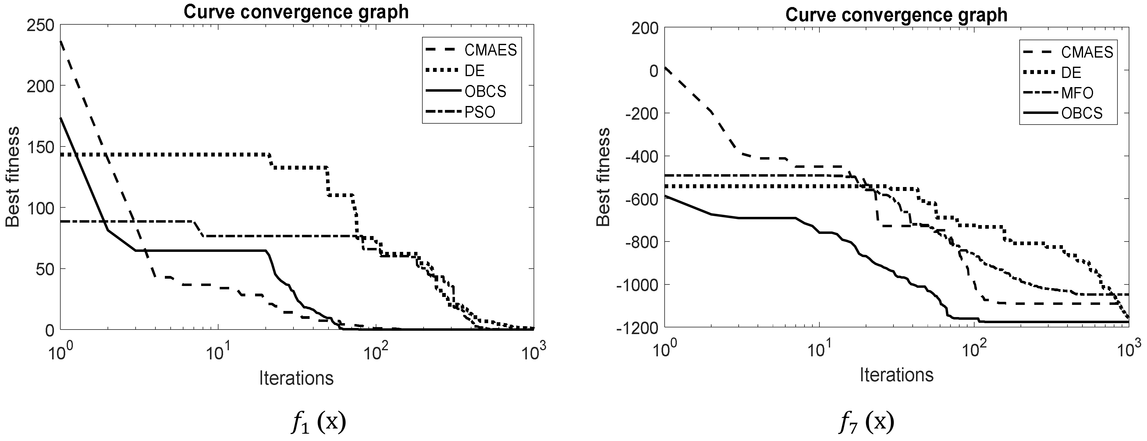
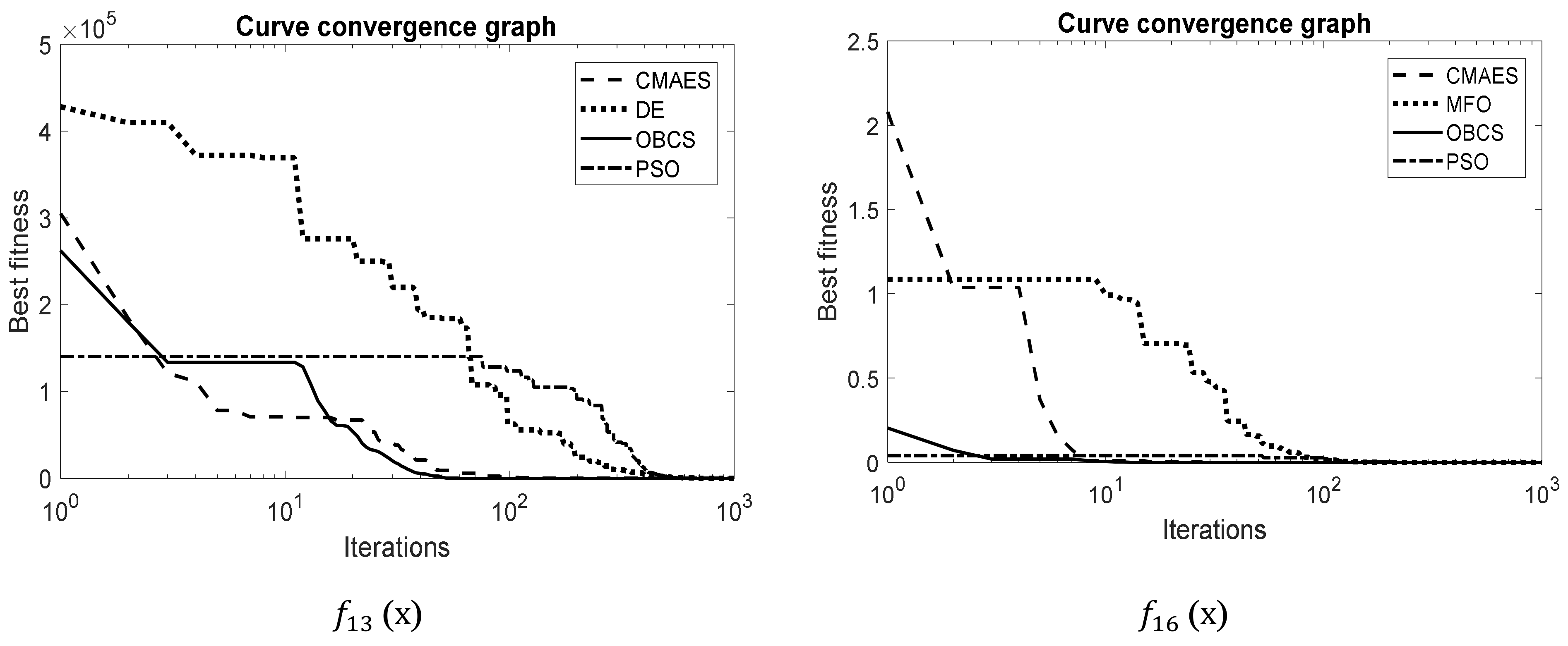
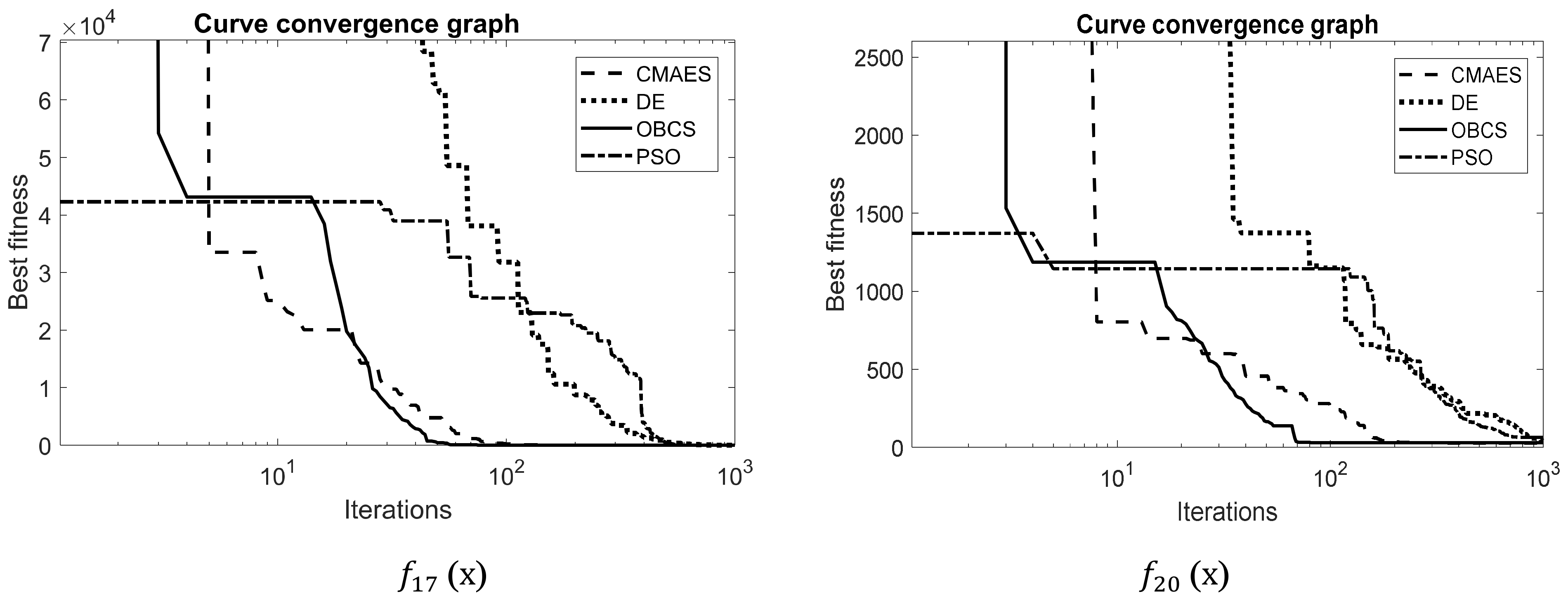
The evaluation of accuracy in the final solution cannot completely assess the abilities of an optimization algorithm. On the other hand, the convergence of a metaheuristic scheme represents an important property to assess its performance. This analysis determined the velocity, which determined metaheuristic scheme reaches the optimum solution. In this subsection, a convergence study has been carried out. In the comparisons, for the sake of space, the performance of the best four metaheuristic schemes is considered adopting a representative set of six functions (two multimodal, two unimodal and two hybrids), operated in 30 dimensions. To generate the convergence graphs, the raw simulation data produced in the different experiments was processed. Since each simulation is executed 30 times for each metaheuristic method, the convergence data of the execution corresponds to the median result. Figure 6, Figure 7 and Figure 8 show the convergence graphs for the four best-performing metaheuristic methods. A close inspection of Figure 6 demonstrates that the proposed SOA scheme presents a better convergence than the other algorithms for all functions.

7.5. Performance Evaluation with CEC 2017

In this sub-section, the performance of the SOA method to solve the CEC 2017 set of functions is also analyzed. The set of functions from the CEC2017 [36] represents one the most elaborated platform for benchmarking and comparing search strategies for numerical optimization. The CEC2017 benchmarks correspond to a test environment of 30 different functions with distinct features. They will be identified from $F_1\left(x\right)$ to $F_{30}\left(x\right)$. Most of these functions are similar to those exhibited in Appendix A, but with different translations and/or rotations effects. The average obtained results, corresponding to 30 independent executions, are re-registered in

Table 7. Optimization results from benchmark functions of CEC2017.

		ABC	CMAES	CSA	DE	MFO	PSO	SOA
	AB	31,543,508.93	16,816,680,165	62,350,211,795	92,576,614.71	9,869,100,268	5,754,474,631	389,770,985.4
${\mathit{F}}_{\mathbf{1}}\left(\mathit{x}\right)$	MD	31,272,497.07	10,317,001,637	62,180,271,044	90,540,094.66	8,120,831,786	5,716,932,117	348,397,609.3
	SD	11,711,445.55	18,287,769,833	6,701,490,748	19,876,885.3	6,276,129,768	3,760,493,838	175,590,731.3
	AB	4.9441 × 1032	1.9584 × 1042	9.584 × 1043	4.6409 × 1032	1.32094 × 1037	1.8354 × 1043	2.4753 × 1019
${\mathit{F}}_{\mathbf{2}}\left(\mathit{x}\right)$	MD	8.92 × 1031	7.2683 × 1041	5.1378 × 1042	9.165 × 1031	5.8224 × 1031	1.5174 × 1031	4.8076 × 1017
	SD	8.1141 × 1032	3.0961 × 1042	2.7242 × 1044	9.8904 × 1032	5.35797 × 1037	1.0053 × 1044	1.2579 × 1020
	AB	143,585.796	206,258.738	105,227.778	184,983.575	141,570.4456	79,667.257	50,153.7766
${\mathit{F}}_{\mathbf{3}}\left(\mathit{x}\right)$	MD	143,614.585	201,904.141	104,066.094	187,839.624	132,229.1115	69,068.2299	47,032.1654
	SD	17,888.2525	52,000.2984	14,953.9048	27,184.1578	57,378.84773	39,077.8042	20,560.6136
	AB	558.75833	3855.6622	16,385.5764	558.09385	1026.441012	937.069787	547.952065
${\mathit{F}}_{\mathbf{4}}\left(\mathit{x}\right)$	MD	562.142677	3566.57161	16,520.3929	556.117066	856.5465617	890.326594	544.342148
	SD	20.2914617	1429.47447	3040.62335	23.4459834	629.655489	361.015317	20.9881356
	AB	730.381143	825.655628	951.170114	721.540918	692.7089629	629.566432	631.994737
${\mathit{F}}_{\mathbf{5}}\left(\mathit{x}\right)$	MD	732.333214	847.872393	951.759754	720.602523	694.7441044	634.793518	630.746916
	SD	12.7345432	66.2497783	22.7361791	9.29337642	42.18671231	29.110803	26.6185453
	AB	603.83984	669.750895	691.817816	604.901193	632.8602211	612.05324	609.329809
${\mathit{F}}_{\mathbf{6}}\left(\mathit{x}\right)$	MD	603.786524	668.724864	691.322797	604.969262	632.4713596	611.116445	608.748467
	SD	0.60630828	9.3375723	6.33324596	0.550883	8.875276889	5.83130625	2.23326029
	AB	977.074304	889.858004	1868.59237	983.896545	1085.414574	850.625181	933.44086
${\mathit{F}}_{\mathbf{7}}\left(\mathit{x}\right)$	MD	977.307172	899.416046	1847.81046	988.619865	1067.152488	837.191947	939.402368
	SD	13.674818	39.0420544	125.687304	17.0217457	139.9764841	43.9666771	25.6723087
	AB	1033.74747	1047.6713	1181.82055	1023.57155	991.3574401	914.911462	920.212894
${\mathit{F}}_{\mathbf{8}}\left(\mathit{x}\right)$	MD	1035.62163	1026.79246	1181.41759	1023.90313	992.7702619	916.328125	921.260403
	SD	13.5776161	86.6169315	29.0041369	12.1336359	43.34646427	24.9852693	21.5473475
	AB	1926.96476	900	15,096.7081	6434.26285	6487.6152	2436.07714	3251.16746
${\mathit{F}}_{\mathbf{9}}\left(\mathit{x}\right)$	MD	1839.55339	900	15,358.9047	6327.72188	5976.801998	2313.97194	2702.63581
	SD	333.208904	0	1637.81695	887.500363	2250.718589	920.338184	1462.45439
	AB	8559.09425	8026.51416	8695.92279	7235.23129	5260.902021	5136.84827	4524.56624
${\mathit{F}}_{\mathbf{10}}\left(\mathit{x}\right)$	MD	8598.36183	7995.60926	8710.13364	7246.56367	5291.679788	4941.91541	4512.99611
	SD	327.683849	246.346496	312.712801	234.084094	711.3287215	845.232077	357.978315
	AB	1594.97778	19,382.0122	7888.11046	1813.68615	4011.754904	1465.88225	1248.42954
${\mathit{F}}_{\mathbf{11}}\left(\mathit{x}\right)$	MD	1594.04404	18,978.0433	7566.7015	1774.91924	2427.207284	1465.34072	1247.83322
	SD	90.044155	9762.53738	2030.84932	246.845029	3525.449844	125.920596	32.5337336
	AB	22,035,530.6	4,281,754,760	8,661,838,227	92,723,516.6	91,292,958.57	354,557,569	4,401,381.17
${\mathit{F}}_{\mathbf{12}}\left(\mathit{x}\right)$	MD	20,991,516.3	4,358,279,185	8,610,836,607	93,208,101.7	23,663,273.6	246,467,712	3,700,514.39
	SD	7,163,344.91	1,489,535,737	2,020,262,530	18,696,916.2	134,545,916.4	411,606,206	3,405,855.44
	AB	19,266.9698	3,652,661,382	6,874,450,894	3,979,238.98	38,881,437.05	111,741,897	26,817.0052
${\mathit{F}}_{\mathbf{13}}\left(\mathit{x}\right)$	MD	18,527.1646	3,905,472,944	7,021,073,065	3,726,551.68	186,879.0885	4,517,059.75	16,966.594
	SD	9421.82494	1,271,069,390	2,248,014,249	1659,861.04	193,180,811.6	371,472,002	23,502.6252
	AB	131,154.772	6,816,811.85	2,093,007.76	270,517.596	369,042.9999	333,813.274	38,907.1977
${\mathit{F}}_{\mathbf{14}}\left(\mathit{x}\right)$	MD	109,800.311	5,506,707.5	1,692,106.9	248,357.925	137,669.8479	99,365.0474	24,004.7416
	SD	74,612.9136	4,656,160.18	1,375,028.96	113,787.245	640,038.5333	1,180,870.46	40,344.6637
	AB	8915.09332	519,343,539	512,525,748	522,995.483	58,693.31574	86,213.8881	7888.58976
${\mathit{F}}_{\mathbf{15}}\left(\mathit{x}\right)$	MD	5428.6522	428,173,625	475,300,661	514,399.613	35,343.82469	63,456.3421	3430.78723
	SD	12,023.8419	350,472,927	266,935,668	282,908.145	74,805.66654	61,784.9118	8715.94813
	AB	3371.67432	4820.88686	5247.63056	2937.15125	3160.316909	2823.54207	2647.38414
${\mathit{F}}_{\mathbf{16}}\left(\mathit{x}\right)$	MD	3388.42168	4838.74796	5230.02992	2987.83654	3135.128472	2823.76408	2599.69633
	SD	194.740886	282.787939	336.291377	168.503372	330.2217186	407.164335	272.998599
	AB	2395.86777	3482.11031	3378.54815	2177.58318	2441.465302	2294.79893	2174.93599
${\mathit{F}}_{\mathbf{17}}\left(\mathit{x}\right)$	MD	2389.4562	3468.22585	3372.19373	2187.84011	2454.470182	2268.3003	2159.79812
	SD	102.889656	285.667211	324.223747	85.3307491	250.2293907	294.2882	194.053384
	AB	5,046,671.6	37,362,365	23,998,373.2	2,228,087.66	4,549,050.542	1,341,517.26	818,677.628
${\mathit{F}}_{\mathbf{18}}\left(\mathit{x}\right)$	MD	4,728,588.97	33,258,799.8	22,232,367.5	2,033,807.45	1,182,780.284	682,252.246	300,231.736
	SD	2,468,179.06	22,078,270.5	13,062,667.1	914,951.248	9,866,226.402	1,857,506.17	1,622,268.27
	AB	16,681.7816	620,387,919	616,153,747	551,809.083	16,702,987.12	13,973,268.1	4686.90195
${\mathit{F}}_{\mathbf{19}}\left(\mathit{x}\right)$	MD	7134.24743	509,584,907	600,010,030	481,336.814	143,655.9903	541,084.259	3334.90276
	SD	24,639.1966	466,495,950	315,926,138	399,361.441	46,487,264.39	44,969,899.6	3974.19763
	AB	2776.66582	2804.5126	2945.57725	2439.77572	2697.417352	2452.70485	2439.26615
${\mathit{F}}_{\mathbf{20}}\left(\mathit{x}\right)$	MD	2764.33673	2834.35184	2955.48441	2445.1877	2627.891978	2488.70557	2449.42599
	SD	94.7983596	199.062724	106.815418	88.0385339	220.4185834	179.132846	147.240337
	AB	2523.44927	2641.22467	2739.23609	2514.75813	2506.000485	2434.7453	2421.58999
${\mathit{F}}_{\mathbf{21}}\left(\mathit{x}\right)$	MD	2524.34506	2643.05906	2741.53087	2518.37232	2499.78219	2433.21201	2426.23287
	SD	15.4046594	36.2479731	41.9080485	10.9762507	40.05305083	23.6970887	21.141776
	AB	4836.58643	9577.04104	9095.47501	6970.19197	6645.22701	5532.20097	4165.49182
${\mathit{F}}_{\mathbf{22}}\left(\mathit{x}\right)$	MD	4242.35722	9932.08496	9075.49459	6750.16911	6848.788542	6523.54829	3767.22155
	SD	2051.83573	1437.66121	763.435864	1310.37051	1508.145086	1932.03672	1801.85242
	AB	2872.69194	3047.39462	3398.54677	2848.15024	2821.343894	2904.06627	2785.54406
${\mathit{F}}_{\mathbf{23}}\left(\mathit{x}\right)$	MD	2872.47313	3045.83859	3425.04431	2848.07645	2814.326953	2917.30159	2781.95288
	SD	10.9306383	35.8015482	80.91846	9.83856624	34.39809682	57.5467798	22.306126
	AB	3029.76315	3180.2796	3622.26109	3048.38906	2970.576725	3097.14113	2998.32425
${\mathit{F}}_{\mathbf{24}}\left(\mathit{x}\right)$	MD	3029.47271	3188.3269	3620.25868	3050.32895	2969.979831	3072.58458	2996.90489
	SD	12.2834187	30.8119037	99.4471973	14.170605	27.40350786	61.1357559	35.0296809
	AB	2918.77003	3333.22102	6228.94202	2976.74179	3234.960327	3006.6561	2931.4471
${\mathit{F}}_{\mathbf{25}}\left(\mathit{x}\right)$	MD	2919.85456	2980.52118	6253.4295	2977.53996	3142.80023	2992.45175	2927.85824
	SD	9.81487821	759.162584	864.95632	16.7265818	310.0654881	102.116534	17.6935953
	AB	5896.23764	8340.37382	11,171.1937	5643.82962	5776.420284	5702.64017	4464.46857
${\mathit{F}}_{\mathbf{26}}\left(\mathit{x}\right)$	MD	5889.23731	8393.26188	11,286.1812	5659.37067	5796.165191	5707.34766	4933.20537
	SD	115.549909	452.740525	720.862035	138.81176	469.5232252	888.194496	945.460049
	AB	3235.30385	3408.04414	4035.72773	3228.08324	3245.912414	3361.79871	3225.24773
${\mathit{F}}_{\mathbf{27}}\left(\mathit{x}\right)$	MD	3235.68049	3407.30733	4021.85789	3228.32551	3242.855656	3349.63975	3224.0298
	SD	6.57578664	33.3663071	190.024017	3.10051948	23.16796867	69.4288619	11.3386465
	AB	3328.57792	6580.85938	7194.47112	3389.18088	4365.338523	3623.74347	3292.31393
${\mathit{F}}_{\mathbf{28}}\left(\mathit{x}\right)$	MD	3326.19	6795.88776	7205.84449	3392.76022	4053.737772	3542.19939	3289.42285
	SD	17.9291186	558.703896	801.137793	29.1593474	920.6971447	251.617478	36.390848
	AB	4459.90622	5654.19067	6442.47253	4169.15715	4120.329591	4068.18331	3734.31699
${\mathit{F}}_{\mathbf{29}}\left(\mathit{x}\right)$	MD	4476.48304	5655.83405	6379.40471	4183.03085	4153.333265	4030.03404	3709.79866
	SD	160.899424	250.599138	525.490575	134.81878	272.9470092	334.451062	167.593361
	AB	401,261.311	629,251,110	736,794,634	317,868.587	876,056.4301	2,818,096.31	27,288.2215
${\mathit{F}}_{\mathbf{30}}\left(\mathit{x}\right)$	MD	343,273.6	484,558,438	795,847,326	289,961.292	213,206.5063	1,323,187.36	23,028.0874
	SD	260,605.287	448,734,951	231,471,227	159,645.774	1,156,943.744	3,490,925.37	12,690.9933

. The results are reported in terms of the performance indexes: Average Best fitness (AB), Median Best fitness (MB), and the standard deviation of the best finesses (SD).

According to Table 7, SOA provides better results than ABC, CMAES, CSA, DE, MFO and PSO for almost all functions. A close inspection of this table reveals that the SOA scheme attained the best performance level, obtaining the best results in 22 functions from the CEC2017 function set. Likewise, the CMAES presents second place, in terms of most of the performance indexes, while DE and CSA techniques reach the third category with performance slightly minor. On the other hand, the MFO and PSO methods produce the worst results. In particular, the results show considerable precision differences, which are directly related to the different search patterns presented by each metaheuristic algorithm. This demonstrates that the search patterns, produced by second-order systems, are able to provide excellent search patterns. The results show good performance of the proposed SOA method in terms of accuracy and high convergence rates.

8. Analysis and Discussion

The extensive experiments, performed in previous sections, demonstrate the remarkable characteristics of the proposed SOA algorithm. The experiments included not only standard benchmark functions but also the complex set of optimization functions from CEC2017. In both sets of functions, they have been solved in 30 dimensions. Therefore, a total of 50 optimization problems were employed to comparatively evaluate the performance of SOA with other popular metaheuristic approaches, such as ABC, CMAES, CSA, DE, MFO and PSO. From the experiments, important information has been obtained by observing the end-results, in terms of the mean and standard deviations found over a certain number of runs or convergence graphs, but also in-depth search behavioral evidence in the form of exploration and exploitation measurements were also used.

The generation of efficient search patterns for the correct exploration of a fitness landscape could be complicated, particularly in the presence of ruggedness and multiple local optima. A search pattern is a set of movements produced by a rule or model that is used to examine promising solutions from the search space. Exploration and exploitation correspond to the most important characteristics of a search strategy. The combination of both mechanisms in a search pattern is crucial for attaining success when solving a particular optimization problem.

In our approach, the temporal response of second-order system is used to generate the trajectory from the position of $x_i^k=\left\{x_{i,1}^k,\dots ,x_{i,d}^k\right\}$ to the location of $b=\left\{b_1,\dots ,b_d\right\}$. Three different search patterns have been considered based on the second-order system responses. The proposed search patterns can explore areas of considerable size by using a high rate of velocity and the same time, refining the solution of the best individual $b$ by the exploitation of its location. This behavior represents the most important property of the proposed search patterns. According to the results provided by the experiments, the search patterns produce more complex trajectories that allow a better examination of the search space.

Similar to other metaheuristic methods, SOA tries to improve its solutions based on its interaction with the objective function or on a ‘trial and error’ scheme through defined stochastic processes. Different from other popular metaheuristic methods such as DE, ABC, GA or CMAES, our proposed approach uses search patterns represented by trajectories to explore and exploit the search space. Since SOA employs search patterns, it presents more similarities with algorithms such as CSA, MFO and GWO. However, the search patterns used in their search strategy are very different. While CSA, MFO and GWO consider only spiral patterns, our proposed method uses complex trajectories produced by the response of second-order systems.

9. Conclusions

A search pattern is a set of movements produced by a rule or model, in order to examine promising solutions from the search space. In this paper, a set of new search patterns are introduced to explore the search space efficiently. They emulate the response of a second-order system. Under such conditions, it is considered three different responses of a second-order system to produce three distinct search patterns, such as underdamped, critically damped and overdamped. These proposed set of search patterns have been integrated as a complete search strategy, called Second-Order Algorithm (SOA), to obtain the global solution of complex optimization problems.

The form of the search patterns allows for balancing the exploration and exploitation abilities by efficiently traversing the search-space and avoiding suboptimal regions. The efficiency of the proposed SOA has been evaluated through 20 standard benchmark functions and 30 functions of CEC2017 test-suite. The results over multimodal functions show remarkable exploration capabilities, while the result over unimodal test functions denotes adequate exploitation of the search space. On hybrid functions, the results demonstrate the effectivity of the search patterns on more difficult formulations. The search efficacy of the proposed approach is also analyzed in terms of the Wilcoxon test results and convergence curves. In order to compare the performance of the SOA scheme, many other popular optimization techniques such as the Artificial Bee Colony (ABC), the Covariance matrix adaptation evolution strategy (CMAES), the Crow Search Algorithm (CSA), the Differential Evolution (DE), the Moth-flame optimization algorithm (MFO) and the Particle Swarm Optimization (PSO), have also been tested on the same experimental environment. Future research directions include topics such as multi-objective capabilities, incorporating chaotic maps and include acceleration process to solve other real-scale optimization problems.