Airborne Electromagnetics to Improve Landslide Knowledge in Tropical Volcanic Environments

Abstract

Caribbean areas are particular volcanic territories in tropical environments. These territories juxtapose several landslide-prone areas with different predisposing factors (poorly consolidated volcanic materials, superimposition of healthy materials on highly weathered materials, high heterogeneity of thicknesses, etc.). In these environments, where rapid development of slopes and land use changes are noticeable, it is necessary to better characterize these unstable phenomena that cause damage to infrastructure and people. This characterization has to be carried out on the materials as well as on the initiation conditions of the phenomena and requires complementary investigations. This study, focusing on La Martinique, proposes a landslide analysis methodology that combines new information about landslide-prone materials acquired by an airborne electromagnetics survey with a physical-based model. Once the data are interpreted and compared with field observations and previous data, a geological model is produced and introduced into the physical model to test different instability scenarios. The results show that geophysical investigations (i) improve the knowledge of the internal structure of landslides and surficial formations, (ii) specify the spatial limits of the materials that are sensitive to landslides, and (iii) give a better understanding of landslide initiation conditions, particularly hydrogeological triggering conditions.

1. Introduction

Landslides are ubiquitous phenomena in the Caribbean [1,2,3,4,5,6], particularly in La Martinique [7,8,9]. With more than 600 events [10,11], this territory is the most affected area in the French Caribbean islands [8]. Phenomena can be shallow, deep, rotational, translational, or complex. The many landslides in the Caribbean are mainly due to the following reasons:

(i)

A complex lithology with heterogeneous volcanic materials that are sometimes poorly consolidated and superimposition of healthy materials on highly weathered materials [12,13,14,15,16];

(ii)

Hurricane and tropical storms associated with intense end heavy rainfalls [1,11,16,17].

Landslides regularly strike the coasts and the hinterlands, and because the island has much built-up land, resulting in anarchic development of the slopes [10,18], landslides can generate damage to the population and infrastructure, creating high rehabilitation costs [8]. Among the most remarkable recent events was (i) the Bellefontaine collapse (vol. = 15 × 10⁴ m³) in 1991 [18], which required €7 million in work to rehabilitate the slope after the event, and (ii) the Morne Callebasse landslide (vol. = 2 × 10⁵ m³) in 2011, which destroyed more than 20 buildings and the road ‘RD 48′, bringing 75 expulsions and more than €17.1 million in works [15,18]. Therefore, anticipating landslides and improving their prevention in this French overseas territory has become a major challenge [8,15].

The first step in achieving these actions consists of assessing hazards [19,20,21]. Several methods that are more or less complex and range from qualitative to quantitative can be used. A large review of their uses can be found in the scientific literature [19,20,21,22,23], and some of them are particularly suited to the French regulatory context [24]. Among them, methodologies using physical-based models (PBMs) at the site scale (<1:5000) are the only methods designed for works [25] or that modified and revised existing regulatory hazard maps, taking into account triggering factors [24]. At this scale of work, it is possible to reach a good understanding of the mechanisms and probabilities of failure or to analyze the runout phenomena by taking into account physical processes. However, in Martinique, the parametrization of PBMs can be difficult because of a lack of information about the nature and depth of materials. Indeed, the island presents a very complex geology with different types of lavas deposited from the Oligocene to the present and exhibits extreme spatial variability and heterogeneity with a high degree of weathering [26,27,28,29,30].

Geophysical investigations can be an alternative to classical field investigations (i.e., geotechnical surveys; [31,32]) to obtain quick information about grounds in large areas. These investigations presuppose correlations between measured properties and physical or geotechnical characteristics [33,34]. In the case of landslides, it is possible to delineate the body of the moving mass of stable grounds due to the changing geophysical parameters [34,35]. However, with heterogeneous grounds, the indirect information that is provided can be biased or difficult to interpret. Therefore, calibrating them with direct observations is indispensable [31], thereby limiting investigations in time and space for very large areas [32].

Airborne electromagnetics (AEM) provides information on lithology and regolith over large surfaces and/or hard-to-access areas [36,37,38,39,40]. It is able to provide plentiful pseudo-3D information about geological structures reaching a few hundred meters [41,42] and has been successfully used in many environmental studies [30,43,44,45,46,47] particularly in volcanic settings. AEM is therefore useful to analyze the internal structure of large landslides [48,49,50,51].

In 2013, an AEM survey was conducted over Martinique Island [52]. The SkyTEM system was designed for mapping geological structures and for hydrogeological and environmental investigations [53]. AEM data, acquired along flight lines, provide information to a depth of 150 m and allow continuous and homogeneous imagery of resistivity variations [30]. If the subsurface resistivity has an indirect relationship with the soil characteristics [31], it can also provide relevant information on both formation thicknesses and their spatialization [32]. To be fully relevant, correlation with direct observations or independent geological datasets (outcrop, borehole geological log, etc.; [31,32]) remains mandatory. Recently, in the framework of future development [15], there has been demonstrated interest in AEM to delineate landslide-prone areas and to improve landslide hazard assessment. New information brought by AEM has allowed a landslide hazard map to be modified by combining a 3D geological model derived from a joint analysis of field observations and AEM results and a PBM. This study, for regulatory purposes, focused on only one type of island environment and on shallow (failure < 2 m) and moderately deep-seated landslides (failure from 2 m to 10 m). Therefore, deeper landslides (failure > 10 m) and associated formations inducing recurrent and very costly damage were not assessed. Considering these results and despite an exhaustive inventory and landslide hazard maps available for the entire island, there is still a lack of knowledge about (i) the nature of certain landslide-prone materials and (ii) the failure mechanisms and triggering conditions for landslides with different failure depths. This work suggests a landslide analysis methodology that combines information about regolith and bedrock derived from AEM results with a spatialized PBM (SPBM) adapted for different types and depths of failures.

Two different areas that are well known for different recurrent slope instabilities, are typical of the island and have caused significant damage for more than 20 years, were chosen to challenge the methodology. The latter is divided into 3 main steps:

• Definition of the internal structure of grounds by coupling field observations, geological data and AEM results;
• Building of a geological model;
• Integration of the topography and geological model in a SPBM and analysis of slope stability following a specific protocol taking field observations into account.

The test sites have benefited from previous field, geophysical and geotechnical studies [54,55,56,57,58,59,60,61,62,63,64,65]. These studies enable (i) a criticism of the AEM results and their interpretation and (ii) the development of realistic failure scenarios based on historical observations and measurements.

2. Martinique and Study Sites

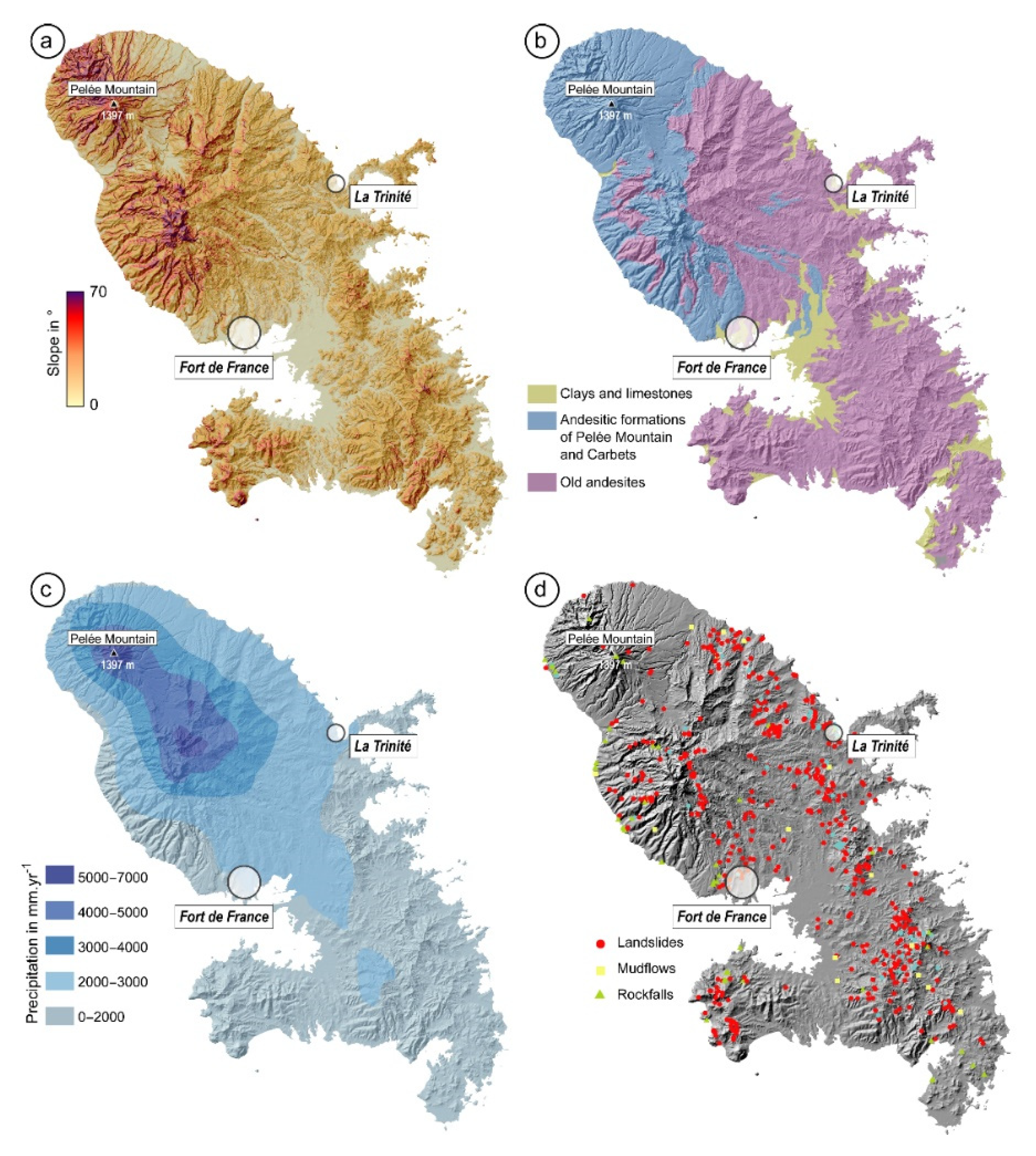
2.1. Generalities

Martinique is part of the French West Indies or the Lesser Antilles (Figure 1a) and results from the westward subduction of the Atlantic plate under the Caribbean plate [26,27]. As the largest island of the archipelago (i.e., 1080 km²), it can be divided into two parts: that with mountainous relief in the north (with Pelée Mountain, a.s.l. 1397 m) and that with a gentler slope in the south (Figure 1a). Orographic effects control rainfall; for instance, the average annual precipitation in the northern part ranges from 5000 to 6500 mm.yr⁻¹ at the highest elevations and from 1200 to 1500 mm.yr⁻¹ in the southern part (Figure 1c). Because the climate is characteristic of a humid tropical climate, a humid season from July to November and a dry season from January to April can be delineated. The annual temperature varies between 18 °C and 32 °C at Fort de France.

2.1.1. Geology

In terms of the geological history, this island is unique because it is located between the old volcanic arc to the east and the recent volcanic arc to the west. Due to this specific position, it is possible to study the chronology of the volcanic front in detail [29]. Starting more than 25 Ma, the volcanic history is complex with alternating eruptive and marine sedimentation phases [26,27,28,29]. These successions allowed the edification of volcanic complexes, which were weathered and dismantled by erosion [30]. Figure 1b gives an overview of the old and recent volcanic deposits.

2.1.2. Landslides

More than 600 landslides have been inventoried during the last 20 years (Figure 2a). They are reported in the French National database (i.e., BD-MVT; https://www.georisques.gouv.fr/ accessed on the 18 May 2020). Each phenomenon is recorded with a minimum set of information, such as the date, the location of the event (centroid in the local geodesic system), the type of formation involved (lithology and/or regolith), and the associated damage, if any. Three types of landslides can be depicted: (i) landslides (i.e., debris slides, rotational and translational slides), (ii) mudflows, and (iii) rockfalls. Figure 1d gives an overview of the location of each phenomenon. Among the different landslides, seven are the subject of special attention because they have generated some damage, and they may continue to generate damage despite some engineering works [8,10].

2.2. Study Sites: Presentation and Previous Works

The two selected sites, which are located in the municipalities of Fort-de-France and La Trinité (Figure 2a and Figure 3), are characteristic of the observed landslides over 20 years and still regularly generate damage despite works and monitoring systems. The two sites have benefited from various geomorphological, geophysical and geotechnical studies that can help guide the various interpretations resulting from airborne electromagnetic surveys.

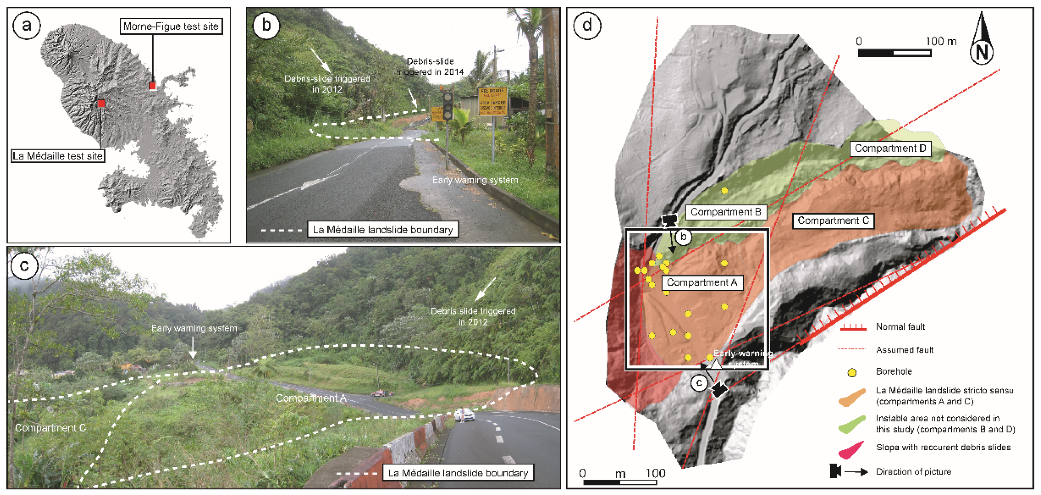
2.2.1. La Médaille Landslide

The La Médaille landslide is located in Morne Balthazar to the north of the Fort-de-France Municipality (Figure 2a and Figure 3a). With a volume of approximately 260,000 m³ and an area of approximately 8 ha (

Table 1. Investigations and monitoring of the two sites since the 1960s.

	La Médaille Landslide		Morne-Figue Area
	Number (n)	Year	Number (n)	Year
Boreholes	15	1966, 1968, 1974, 1981, 1986, 1996	9	1981, 1982 1989, 1997
Geotechnical characterization	2 campaigns	1981, 1983	1 campaign	1989
Geophysical investigations	1 campaign (AEM)	2013	2 campaigns (electrical and AEM)	2007, 2013
Hydrogeological investigations	2 periods	Precipitation= since 1969 Piezometer = 2000 and 2002	1 period	Precipitation 1988–1989 Piezometer = 1988–1989
Field investigations	9 campaigns	1966, 1968, 1974, 1981, 1986, 1996, 2002, 2014, 2016	7 campaigns	1981, 1982 1989, 1997, 2007, 2016, 2017

), the landslide occurred in 1916 [54,55], removing the old village of La Médaille and causing five casualties. The landslide is bounded to the north and south by two water courses marking two parallel faults and by a cliff of approximately 110 m representing a normal fault in the west. It is probably located on a paleolandslide (rock avalanche) represented by dacitic deposits in the small-scale lithological map [26,27]. Since 1916, several peaks of activity have been recorded (i.e., 1958, 1966, and 1993; [54,55,56,57,58,59,60,61,62]), each time with the rehabilitation or the relocation of road RN3 due to its crossing the moving mass. It is a slow-moving landslide but is likely to experience accelerations due to GWL variations. More recently, a debris slide in weathered andesitic formations occurred in the upper part of the cliff overhanging the landslide (Figure 2b,c).

Since the 1960s, several investigations (i.e., field surveys, geotechnical studies, and monitoring; Table 1) were engaged to improve the knowledge of the landslide [54,55,56,57,58,59,60,61,62,63], especially for the upper part (compartment A). Indeed, the topography of the lower part (compartment C) of the landslide is chaotic and complex, and the very dense tropical vegetation prevents the deployment of different investigation devices. The different field surveys allowed delineation of four main compartments functioning more or less independently. The lower compartment (C) seems to have an influence on the upper compartment (A), while the compartments on the edges are considered independent of the main landslide stricto sensu [58]. All drilling campaigns (five campaigns between 1967 and 1996) were located in compartment A of the landslide, which presents a high blockage potential (Figure 2). Thus, this compartment benefited from 14 boreholes reaching a depth of approximately 20 m. These campaigns located the faults bordering the landslide (Figure 2d).

The first campaign in 1967 revealed a more or less clayey upper layer, up to 3 m thick, followed by approximately 19 m of dacitic screes upstream and 3 m of dacitic screes downstream of compartment A (Figure S1). Under this layer, a thin clay layer of a thickness of 0.5 to 0.9 m was observed. Finally, the lower layer was interpreted as andesite bedrock that was more or less fractured [54,55]. Hazmoune et al. [57] questioned this statement following new observations based on new boreholes. Indeed, the last layer would be a mixture of weathered andesites and breccias and could be part of the landslide, which would then be composed of two superimposed bodies. This information corroborates the conceptual scheme of landslide development established in [56,57,63], which mentioned the implementation of a rock avalanche in andesites. This layer would have been weathered and would then have been covered by a thick layer of dacite debris (breccias), which would have also been weathered.

The different boreholes defined a groundwater level between 1967 and 1968 in the upper part of the landslide with a maximum piezometric level of approximately 10 m under the topography. The fault system and a nearby spring probably feed this water level [57]. Finally, a series of rainfall and piezometric records attempted to prove the relationship between precipitation, groundwater level (GWL) and landslide activity. Unfortunately, despite the punctual implementation of a measurement network, shortcomings in the precipitation series or in displacement monitoring did not allow this relationship to be clearly proven. Nevertheless, when the GWL is high, the activity of landslides increases [54,55,57].

2.2.2. Morne-Figue Area

The Morne-Figue area is located in the commune of La Trinité on the east coast of the island (Figure 3b). The study site covers an area of 0.36 km² and is limited to the north and west by the Morne-Figue (129 m a.s.l.) and the Morne-Congo (232 m a.s.l.) areas, respectively, which are carved in compact andesite, to the south by the Gué stream and to the east by Crosmy Bay. The site is hilly with elevations varying between 10 m and 100 m a.s.l. and both steep and gentle slopes varying between 5° and 45°. The site, which is very anthropized (approximately thirty houses), is bordered to the west by national road RN1 and is crossed by a small road connecting the neighborhood to the center of the municipality (Figure 2c,d). Since 1977, the east-facing slope has been subject to landslides (rotational and shallow translational landslides). The main phenomena is located below RN1. This landslide, which is approximately 2.99 ha and was triggered in 1988 [64], is associated with rotational failure in the upper part and a translational component in the lower part ([64]; Figure 3d). This phenomenon has two very active periods: from 1987 to 1988 and in 2004. Since 2004, new geomorphological features such as cracks (i.e., traction and compression), small scarps and new tension cracks on the road were observed intermittently (Figure 3).

One drilling campaign [64] and geophysical investigations allowed the involved materials and their thicknesses to be defined (Figure S2). Four types of formations from the topographic surface were defined: (i) an upper layer composed of clays or backfill with a thickness between 1 m and 3 m; (ii) a second layer with a thickness from 8 m to 10 m and represented by weathered very clayey materials; (iii) a third layer with a thickness between 10 m and 12 m composed of weathered basalts (Pré-vert basalts); and (iv) a weak horizon of basalt whose thickness is not known. A piezometer was implemented for the period of 1987–1988. During the humid period (from May to October), the GWL lies between 1.4 m and 0.5 m below the topography from upstream to downstream. In the dry season, the GWL is approximately 8 to 9 m below the topography. The piezometric levels and displacement measurements were implemented for a short period of one year, showing a correlation between rainfall and landslide activity [64]. Consequently, the landslide was more active during the humid period, with a maximum displacement of approximately 1.4 cm for the period of 1987–1988. In 2016, the geological knowledge of the surroundings was refined by field observations along cross-sections. Beyond the acquisition of new geological information, two units within the landslide were delineated with a very active unit upstream and a latent unit downstream. New shallow parallel landslides were observed within the site.

3. Materials and Methods

The suggested methodology is based on a transdisciplinary approach in three steps. This approach reduced the uncertainties raised by previous studies, particularly concerning the internal structure of the La Médaille landslide and the different material types and thicknesses of the Morne-Figue area. The interconnected steps are (i) the identification and improvement of the knowledge of involved materials; (ii) the production of a geological model for each site, including the different regolith thicknesses and/or internal structures of landslides; and (iii) landslide susceptibility analysis by a spatialized physically based model based on limit equilibrium equations with research of best fitting geotechnical parameters. Step (iii) integrates empirical triggering factors according to field observations.

3.1. AEM Data

From 29 January to 16 March 2013, SkyTEM ApS conducted a survey over Martinique Island. This survey, supervised by the BRGM (French Geological Survey) and totaling 4233 line-kilometers, was flown along the N–S direction with a 400-m spacing; locally, this spacing was refined to 200 m over areas of interest for the hydrogeology or risk assessment [52]. Along each line, EM measurements were spaced approximately 30 m apart, with an average ground clearance of approximately 64 m due to the sharp topography of the island. Figure 4 shows the location of the flight lines flowing over the two studied sites.

SkyTEM is an AEM system developed by the Hydro Geophysics Group of Aarhus (Denmark) for hydroenvironmental investigations [53]. This system is composed of (1) a transmitter coil exciting the subsurface, (2) a receiver coil to measure the ground response, (3) a generator as a power source, and (4) several navigation instruments, such as GPS, tiltmeters, and laser altimeters, to locate the loop in space. The SkyTEM system operates in dual transmitter mode. The low moment, with a magnetic moment of approximately 2826 Am² and time gates from 11 µs to 1 ms for the present survey, provides early time data for shallow imaging, and the high moment, with a magnetic moment reaching 144,440 Am² and time gates from 109 µs to 8.9 ms, allows measuring later time data for deeper imaging. Locally, the depth of investigation of the method depends on the emitted magnetic moment, the bandwidth used, the subsurface electrical conductivity, and the signal/noise ratio.

The AEM method allows imaging of the conductivity contrasts of the subsurface. To obtain usable measurements, several processes are applied to remove couplings with man-made installations and ambient noise from the signal. The processing scheme used is described in [39,40] and is based on singular value decomposition [39,40]. Data are then inverted using the spatially constrained inversion algorithm (SCI) [44]: (i) each usable AEM measurement is translated into a 1D (EM sounding) model divided into n layers, each defined by its thickness and resistivity, and the resistivity variations are displayed according to depth; during the inversion, constraints are applied vertically and spatially between nearby soundings (independently of flight lines). (ii) The ground clearance of the AEM system is also inverted, and the depth of investigation (DOI) is assessed as a final step in the inversion [66]. The results were obtained by running a smooth inversion for 25 layers from 0 m to 300 m deep. Each layer has a fixed and equal thickness. Only the resistivity values vary within a layer [39]. This approach is effective for imaging complex geological structures with the lowest dependency on the starting model, but it only displays a smoothed view of the subsurface. At this step, each flight line can be displayed as a resistivity profile composed of all the associated EM soundings. More 2D information can be obtained by interpolating, on raster grids, the resistivity of layers falling into a depth or elevation range. This interpolation is generally repeated to obtain slices over the entire range of investigations. Slices can then be merged to obtain a 3D resistivity model [45], (i) drawing profiles in any direction for confronting geological data (maps, boreholes, and field observations) and (ii) deriving interfaces for each imaged horizon.

3.2. Interpretations and Conceptualization

3.2.1. Confrontation with Independent Data

To interpret the different imaged horizons for defining interfaces of interest, a comparison with boreholes and field observations is carried out (Figure 2 and Figure 3) by projecting the geological data on selected resistivity profiles. The distances between the boreholes and AEM lines vary from 2 to 10 m and 3 to 12 m for the La Médaille landslide and Morne-Figue area, respectively.

3.2.2. Geological Modeling

Based on interpreted resistivity profiles, boreholes, geological maps and field observations, a geological model is produced for each site [67,68]. AEM results are useful to constrain the model for different environments [37,38,41]. The principle is based on the first two steps of the approach described in [67] and the different positions of geological limits (contacts between two geological formations or lithologies). They are used to guide the interpolation by the kriging method as regular grids representing the bottom of each type of identified formation.

3.3. Landslide Modeling

3.3.1. ALICE Presentation

Landside modeling is performed with ALICE^® (Assessment of Landslide Induced by Climatic Events) developed by the French Geological Survey (BRGM, [69]). This tool supports landslide susceptibility mapping for areas ranging from local sites (catchments) to large areas (several municipalities; [15,69,70,71]). Developed in a GIS environment (MAPINFO^®), it is a SPBM described in [69] and summarized below (Figure 5).

The geometry of the studied area is introduced in raster format with (i) the topography and (ii) the geometry of different material layers. Geomechanical characteristics, cohesion (c), friction angle (φ) and specific bulk unit weight (γ), are given for each lithology and surficial formation. These parameters can be implemented by a constant value or by probabilistic distributions to take into account environmental variability and uncertainties [69,70]. The tool supports different landslide geometries and failures (i.e., rotational, translational, and complex with different lengths and depths). Two triggering factors can be used: (i) the groundwater level (GWL) or (ii) seismic acceleration. The GWL represents the saturation ratio (m = h/z), where h is the height of the water table and z is the depth of the material(s) taken into account. The GWL can be implemented empirically in one or several formations by increasing the saturation level from 0 (dry conditions) to 1 (saturated conditions) or with the help of a hydrogeological model taking into account the effective rainfalls. Seismic acceleration is represented by the peak ground acceleration (PGA).

The slope stability computation is based on a limit equilibrium method (LEM) and slice theory described in [72] and in Figure S1. The iteration process is based on the concept of reducing the number of iterations about the interslice function and therefore the computation time [73]. The hypothetical failure surface is divided into n vertical slices, and each slice I is subject to the normal shear interslice forces and to the shear resistance (Figure S3), where:

$$R_i=\left[w_{i}cos{\alpha }_i-u_i{b}_{i }\sec {\alpha }_i\right]tan{\phi }_i^{\prime }+c_i^{\prime }{b}_i\sec {\alpha }_i$$

and the moving forces:

$$T_i=w_{i^{\sin \alpha }i}$$

where W_i: weight; α_i: base inclination; u_i: average water pressure; b_i: width of the slice; φ_i: effective friction angle; c’_i: cohesion along the base; and R_i: sum of the shear resistances, except the normal shear interslice forces. Ti is the component tending to cause instability. The potential failure is expressed by the factor of safety (FoS). If the FoS is below 1, the slope (i.e., the computation cell) is considered instable. The slope stability assessment is performed on regularly spaced 2D profiles automatically produced over the whole area and based on maximum gradient lines from the DTM. Two types of computation are possible, (i) the computation of the FoS or (ii) the computation of the probability, to obtain an FoS below 1 for each cell. In the second case, the tool performs a random selection of each geotechnical value following probabilistic distributions and Monte Carlo simulations [69,70,71].

3.3.2. Landslide Modeling Protocol

Landslide modeling, split into three steps, consists of defining the best set of representative parameters for each site.

(i)

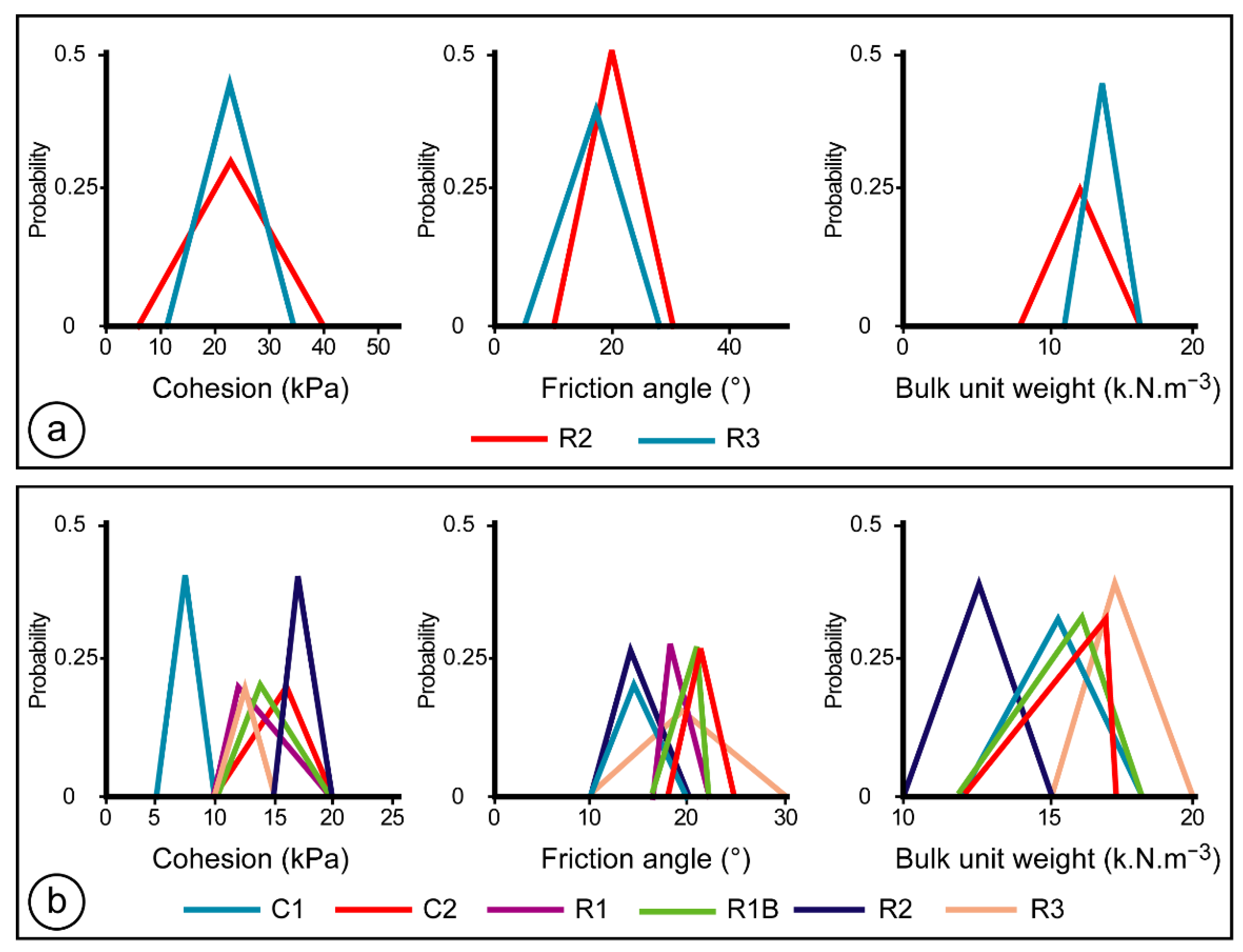
The first step focuses on the geotechnical characteristics acquired during the drilling campaigns at each site. The goal is to reduce the broad spectrum of geotechnical values because their range is quite large. Indeed, retaining geotechnical values giving recurrent instability under any saturation conditions would not be representative of real conditions, with landslides being episodically unstable. Therefore, a sensitivity study is undertaken by several iterations computing the FoS in dry and fully saturated conditions. Computations are carried out in 2D along a representative cross-section of the study site. Each geotechnical characteristic (cohesion, angle of friction, and bulk weight density) is modified iteratively by increasing its value and keeping constant values for the other two. If the results show recurrent instability under any condition (dry/saturated), the value is excluded. If the results show a recurring stability of the sites under any condition (dry/saturated), then this value is also excluded. Thus, by this sensitivity analysis, the values (cohesion, angle of friction, bulk unit weight) producing a factor of safety lower than one at a high GWL are preserved, and those producing a factor of safety greater than one for a null GWL are also preserved.

(ii)

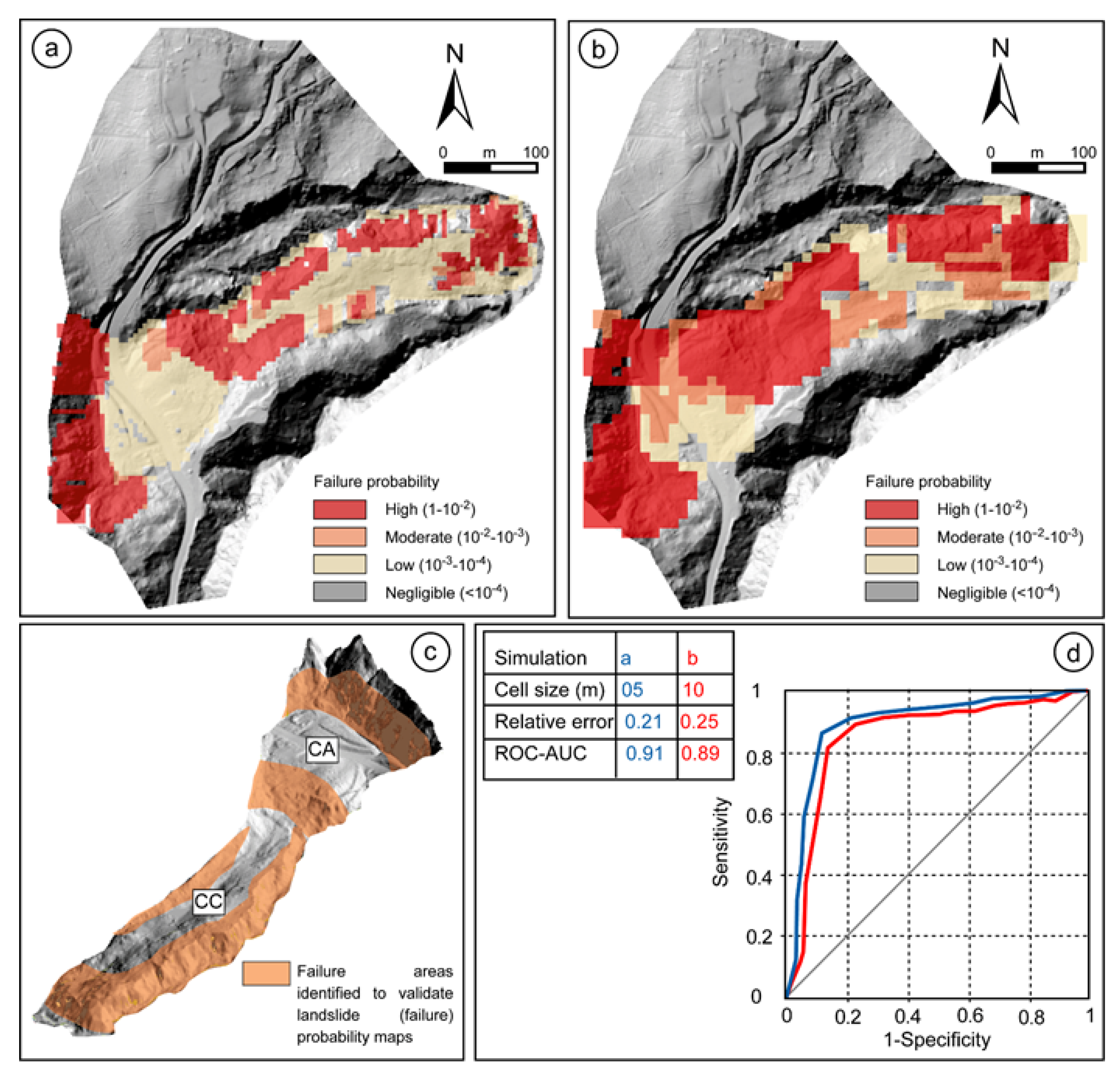
The second step consists of defining the optimum cell size for ALICE^® to obtain reliable results. Indeed, for the spatialized model, in raster format, the cell size can generate errors that propagate in the results [74,75]. Thus, for the two sites, simulations are carried out with cell sizes of 10 m and 5 m to observe if discrepancies can be noted between the simulations. It is not necessary to decrease the resolution because with a lower cell size, the generated profiles are too small, and it is impossible to correctly compute failures shorter than 10 m ([62,69]). Conversely, performing calculations with a larger cell size results in a loss of spatial precision, sometimes generating areas with a low or high failure probability that is not characteristic of the field reality [62]. Computations are performed with the geological models developed with the new data from the AEM data and interpretation. For this step, the best geotechnical values defined previously are used. The GWL introduced in ALICE^® is constant and corresponds to full saturation conditions.

(iii)

The third step allows checking the influence of the GWL on the destabilization of the ground. This step takes into account the GWL recorded for the two sites from 1967 to 1968 and from 1987 to 1988 for the La Médaille landslide and Morne-Figue area, respectively. Therefore, following the different records, the maximum GWL is established with a maximum fixed at −0.5 m from the topography surface for the La Médaille landslide, −0.5 m from the topography surface for the moderately deep rotational landslide and a GWL at the level of topography for the translational shallow landslide for the Morne-Figue area. The different saturation ratios increased iteratively from dry conditions (GWL = 0) to full saturation conditions measured for each site (GWL = 1).

For each step, the failure geometries were fixed following the field observations (

Table 2. Landslide characteristics used for modeling.

	La Médaille	Morne-Figue
Landslide type	Deep	Moderately deep	Shallow
Failure length (m)	45–50	45–50	10–15
Failure depth (m)	20–40	9–10	2–3

). The validation of simulations is performed by comparison with (i) an expert map derived from field observations and DTM derivatives for the La Médaille landslide [62,76] and (ii) the landslide inventory performed in 2016 for the Morne-Figue area [62]. Different classical statistical tests are computed (relative error and ROC-AUC; [69,70,71]) to validate the results. These tests were completed by expert (qualitative) verification.

4. Results

4.1. Identification of Involved Materials and Geological Models

For each site, resistivity profiles and grids (at different depths) were combined with boreholes, field observations and geological maps (Figure 6 and Figure 7). Interfaces of interest were then extracted to constrain the geological model.

4.1.1. La Médaille

Figure 6a,b shows two resistivity grids at two different depths, between 4 and 7 m and between 48 and 47 m deep. For each, the geological formations and the landslide were reported. The dacitic formations (breccias and bedrock) show high resistivity values (>65 Ω.m, Figure 6a). It is possible to observe them in the western part of the landslide. At the level of the landslide, the resistivity values are between 20 Ω.m and 35 Ω.m, corresponding to the dacitic screes observed in the boreholes and described in [58,59] and [61]. Deeper (Figure 6b), high resistivity values (>50 Ω.m) are imaged to the west and northwest of the landslide and correspond to the dacitic formations, whereas the landslide area is characterized by a low resistivity, below 15 Ω.m. A resistivity profile is shown in Figure 7a and is completed in Figure S1. Nearby boreholes are also projected on this profile to identify the different materials (Figure 7a). At the surface, a thin conductive layer (C1) is visible with a resistivity of approximately 15 Ω.m. It would represent the superior clayey layer described in the different boreholes. Under it, a more resistant layer (R2 ~50 Ω.m) can be observed. It is assimilated by the dacitic formations of the old debris avalanche described in [54]. Below R2, a thick layer (R3) with a lower resistivity (from 15 Ω.m to 30 Ω.m) is imaged. This layer is the one observed in Figure 6a and was interpreted as breccias or fossilized screes in [54,55]. The deep conductive thick layer (C2) would correspond to weathered andesite. This conductive layer, present along the landslide (Figure 6b, Figure 7a and Figure S1) and not revealed with the older boreholes, would be 30 m thick and would overcome the bedrock composed of andesite (R4).

Table 3. Characteristics of the different formations observed in the La Médaille landslide.

Name	Resistivity (Ω.m)	Thickness (m)	Description
R1	>50	>20	Very deep layer with high resistivity values corresponding to dacite
C1	15	1–3	Surficial layers corresponding to recent weathered materials rich in clay
R2	50–55	4–20	Layer with high resistivity values corresponding to dacitic screes and debris implemented by an ancient debris avalanche
R3	15–30	20–30	Layer under R2 with lower resistivity values corresponding to mixed materials (breccias or fossilized screes)
C2	<15	25–30	Layer with low resistivity values and a thickness of approximately 30 m corresponding to weathered andesite at the bottom, which was probably caused by hydrothermal water
R4	20–25	not identified	Formation with high resistivity values and likely corresponding to the bedrock (andesite)

details each formation.

4.1.2. Morne-Figue

Figure 6c,d show two resistivity grids at two different depths, between 2 and 4 m and between 19 and 24 m. The resistivity range is globally low (<50 Ω.m). At the surface, the highest resistivity corresponds to andesites and volcanic-sedimentary formations. Weathered basalts have a lower resistivity (< 8 Ω.m). Landslides occur in the majority of these materials described in [62,63]. In between, it is possible to define the hyaloclastites. Resistivity profiles are displayed in Figure 7b and Figure S2. Nearby boreholes are also shown. Six horizons are delineated: a conductive layer (C1; <5 Ω.m) corresponding to a very weathered clayey layer and backfill materials that is more or less saturated following the groundwater level, and a more resistive layer (R1; from 5 Ω.m to 8 Ω.m) corresponding to less weathered clay materials. Locally, this layer disappears in lieu of a more conductive layer C2 (from 2 Ω m to 5 Ω m).

According to borehole data (Figure 7b), this layer (C2) would correspond to highly weathered lavas, where water was observed [63]. C2 disappears progressively downstream of the slope and is less weathered at depth (R4) in favor of a few resistive layers (R1B and R1). Under R1, C1 and R1B, R2 shows higher resistivity values (between 8 Ω.m and 11 Ω.m). This layer, located 25 m below the topographic surface, would correspond to hyaloclastites. However, it remains difficult to know the exact nature of this layer due to the lack of deep boreholes. Finally, a more resistive layer (R3), with values higher than 20 Ω.m, corresponds to andesite formations overlying the hyaloclastite formations in some places. It should be noted that two sectors, where resistivity values drop sharply, probably correspond to faults delimiting the topographic depression at the center of the study site.

Table 4. Characteristics of the different formations observed in the la Morne-Figue area.

Name	Resistivity (Ω.m)	Thickness (m)	Description
C1	<5	2–4	Weathered clayey and backfill materials
C2	1–5	5–10	Highly weathered basalt lavas with preferential water circulation
R1	5–8	3–10	Basalt lavas that are more or less weathered
R1B	5–8	3–10	Basalt lavas that are more or less weathered that are replaced laterally and at depth C2
R2	8–11	15–20	Hyaloclastite formations
R3	>20	>20	Andesite formations that are more or less weathered

gives the different characteristics of each formation.

4.1.3. Geotechnical Models

From the interpreted resistivity models, different interfaces were derived for each site. Figure 8 and Figure 9 illustrate the different geological models for the two sites.

For the La Médaille landslide, four layers were defined (Figure 8a): (i) a first layer corresponding to dacitic screes (R2) upstream of the landslide on steep slopes and on compartment A of the landslide. The thickness varies from a few decimeters to approximately 5 m upstream of compartment A. On compartment A of the landslide, the thickness varies from 5 m to 20 m. (ii) A second layer corresponds to andesite screes (R3) with a thickness between 40 m under compartment A and a few meters downstream of compartment C. Therefore, R2 rests on R3 along compartment A and forms compartment C alone. (iii) A third layer corresponds to dacite (R1) located under R2 up to the concave slope failure corresponding to the upstream limit of the landslide. It is limited downstream by the north-south fault. Its thickness varies from 20 to 90 m. (iv) A fourth layer corresponds to andesite (C2) forming the bedrock. The fault observed in the resistivity profile (Figure 7a) and documented in the geological map [26,27] is not integrated in the geotechnical model. Figure 8a shows the failure hypothesis described in [54] and questioned in [57]. The new information on formations and their thicknesses introduced in the geotechnical model and numerical simulations under ALICE^® should help to better understand how destabilization occurs.

For the Morne-Figue landslide, the area was divided into five homogeneous areas, defined by the main formations identified previously, the structure and the geomorphology (Figure 9a). Thus, S1 corresponds to the hyaloclastite formation (R2) resting on andesite formations (C1); this area corresponds to the main relief. S2 is composed of hyaloclastite (R2) marking steeper slopes. S2 is separated from S3 by a fault identified in the resistivity model and identified in [26,27]. S3 marks the beginning of the topographic depression of the site. It is characterized by a succession of conductive and more resistive layers (C1, R1, C2, and R1B), including the C2 layer over almost its entire surface. S4, in the southern part of the site, differs from S3 by an absence of layer C2 on the entire downstream and eastern part. Therefore, downstream of S4, only C1 and R1 are identified. Area S4 is probably limited to the north by an assumed fault separating it from S3. Finally, S5 represents the downstream of the site with gentle slopes covered by alluvial deposits. Faults in this area are not integrated into the geotechnical model. Numerical simulations with ALICE^® constrained by the new information brought by the AEM (nature and extension of the formations and their thicknesses) allowed spatializing landslide hazards at the study site.

4.2. Slope Instability Analyses

For stability analyses, the best geotechnical parameters to be introduced in the models should be chosen. Moreover, this step tests the contribution of the information derived from the AEM and uses it to build the conceptual models on both the different materials involved and the different destabilization conditions.

4.2.1. Identification of the Best Geotechnical Parameters

The sensitivity analysis along the cross-sections (Figure 8a and Figure 9b) must reduce the range of values of geotechnical parameters and define the consistency as the best fitting intrinsic for the involved materials. A set of 50 model iterations for each cross-section were carried out (i) with independent variation of each parameter within the range of values and (ii) in dry and fully saturated conditions to obtain the best range of combinations.

Table 5. Geotechnical values selected after sensitivity analysis for the La Médaille landslide. IV = initial values; SV = selected values; γ = bulk unit weight; c = cohesion; φ = angle of friction; italic values are introduced as triangular probability distributions in ALICE^®.

Formation	Thickness (m)	γ (kN.m−3)		c (KPa)		φ (°)
		IV	SV	IV	SV	IV	SV
R1	>20	25–30	30	40–50	40	30–50	40
R2	2–20	10–17	11–16	10–37	12–35	5–30	5–25
R3	20–30	7–17	8–16	6–50	6–40	8–35	10–30
C2	25–30	25–35	28	35–40	37	28–47	40

and

Table 6. Geotechnical values selected after sensitivity analysis for the Morne-Figue area. IV = initial values; SV = selected values; γ = bulk unit weight; c = cohesion; φ = angle of friction; italic values are introduced as triangular probability distributions in ALICE^®.

Homogeneous Area	Formation	Thickness (m)	γ (kN.m−3)		c (KPa)		φ (°)
			IV	SV	IV	SV	IV	SV
S1	R3	>20	10–30	15–20	8–16	10–15	5–40	10–30
	Substratum (andesite)	infinite	26–30	30	40	40	40	40
S2	R2	15–20	05–29	10–15	5–20	15–20	1–35	10–18
	Substratum (hyaloclastite)	infinite	29–30	29	31–35	35	31–35	35
S3 and S4	C1	1–3	12–17	12–17	5–15	5–10	10–22	10–20
	R1	3–10 m	10–18	12–18	1–20	10–20	16–25	17–22
	C2	5–12 m	10–18	12–18	5–25	10–20	18–25	18–25
	R1B	3–10 m	10–18	12–18	5–25	10–20	16–25	17–22
	Substratum (basalt)	infinite	25–30/ 29–30	29	50–66/ 31–35	66	30–38/ 31–35	38

give the selected formation and the retained boundaries to perform calculations. For the two sites, cohesion appears to be the most influential parameter in the safety factor modeling followed by the internal friction angle, while the weight bulk density appears to be the least influential, which is often noticed in this type of analysis.

Therefore, for the La Médaille landslide, the results for rotational failure with a depth of 20 m show that the cohesion must not be below 12 KPa and 6 KPa for layers R2 and R3, respectively, especially if the angle of friction is low for each layer. If the value is below one of these values, the computed FoS remains under 1, corresponding to a recurrent instability that does not correspond to reality.

For the Morne-Figue area, there are two cases: shallow and moderately deep-seated landslides. For shallow landslides occurring in the R1 materials, if the angle of friction is higher than 15°, then the slope remains stable. For cohesion, when it is greater than 10 KPa, the slope remains stable. On the other hand, when cohesion is close to 5 KPa, the slope switches from stable to unstable according to the saturation scenario. For moderately deep-seated landslides, the situation is more complex, regardless of the conditions, and the slope is close to instability even with high cohesion values and/or high angle of friction values. When the GWL is low and the saturation conditions are null, then the FoS is high, but not higher than 1.5. Therefore, when the angle of friction is less than 10°, the stability remains low under any condition. If the angle of friction is higher than 20°, the slope is stable. For cohesion under 5 KPa, the slope is recurrently unstable (FoS < 1) regardless of the angle of friction. If the angle is greater than 10°, then according to the angle of friction, the stability increases.

Table 5 and Table 6 show the initial and retained values to be integrated in the spatial modeling for the two case studies. Values in italics are used in ALICE^® simulations. Values in italics and bold are used with a probability distribution necessary to compute failure probabilities with ALICE^®. The probability distributions taken into account are triangular (Figure 10). This shape of the probability distribution is classically selected for ALICE^®, as explained in [69,70], and offers the best compromise for testing new hypotheses of slope destabilizations.

4.2.2. Identification of the Optimum Cell Size

For this step, computations are performed with 10 m and 5 m cell sizes. The geotechnical dataset is the best previously defined for each site. For the La Médaille site, two computations are carried out with rotational failures with a depth of 20 m. For the Morne-Figue site, four computations are performed (two for shallow landslides with a maximum depth of 3 m and two for deep rotational landslides with a depth of 10 m). The goal was to define the best cell size given the best results, and it was decided to perform the computations taking into account the failure conditions observed in the field (i.e., with a high GWL corresponding to the saturation of the materials, GWL = 1). The comparison and validation of the results is carried out by two statistical tests and expert verification. The tests are classical: (i) the relative error analysis (performed with the observed failure identified) and (ii) the analysis of the area under an ROC curve (ROC-AUC). For the La Médaille site, failures correspond to the main scarps of the landslide (i.e., the scarp between compartments A and C and the scarps identified downstream). For the Morne-Figue, failures correspond to scarps of phenomena.

Figure 11 and Figure 12 depict the results for computations carried out with the two cell sizes for each site. For the La Médaille test site, the different scarps are well identified by the models with high probability values of failure in the different scarps. The relative errors are very low, with 0.25 and 0.21 for the 10 m cell size and 5 m cell size, respectively. The two computed ROC-AUCs show that the different models have a high degree of fit with values of 0.89 and 0.91 for a 10 m cell size and a 5 m cell size, respectively. For the Morne-Figue site, for shallow landslides, the different models computed with cell sizes of 10 m and 5 m have a low degree of fit. Indeed, the relative error and ROC-AUC have values of 0.89 and 0.95 and 0.59 and 0.58 for 10 m and 5 m cell sizes, respectively. These results indicate a low degree of model fit and low model representativeness for translational shallow landslides. In contrast, for moderately deep rotational landslides, the results are very good, with low relative errors and high ROC-AUCs of 0.13 and 0.15 and 0.89 and 0.87 for a 10 m or 5 m cell size, respectively. The Morne-Figue failure area is well represented with high probability values from 0.1 and 1, indicating, according to the equations, high failure probabilities when the materials are saturated.

Hillshade maps were produced with the Helimap DTM (2013).

For both cases, the results few differ between computations with a cell size of 5 m or 10 m, either statistically or visually on the computed maps. Thus, for the two sites, a cell size of 10 m appears to be the best compromise for the next phase. For the Morne-Figue site, given the low representativeness of the models, it is necessary to have other information to better adjust the computations. Therefore, the influence of the GWL is not tested for shallow translational landslides.

4.2.3. Influence of the GWL

The initial hypothesis following antecedent monitoring and observations is that the two case studies are controlled by the rise of the GWL corresponding to the material saturation. Therefore, several scenarios were tested by gradually increasing the GWL. The scenarios take into account the best calculation cell size (i.e., 10 m), and the best set of geotechnical data. For the La Médaille landslide, the goal is to find the most favorable materials prone to failures, confirming the landslide-triggered hypotheses. Thus, several scenarios were tested with computations of failures (i) for R2 in dry and completely saturated situations (i.e., GWL = 0 and GWL = 1), (ii) for R3 in dry and completely saturated situations (i.e., GWL = 0 and GWL = 1), and finally, (iii) for both types of materials in dry and completely saturated situations (i.e., GWL = 0 and GWL = 1). Once the materials to be considered have been defined, the influence of the GWL is tested by gradually increasing its level from 0 to 1 (with a maximum at 0.5 m below the topography). For the Morne-Figue area, considering the stakes, the main goal is to improve the knowledge about the material of the compartment face and the rise of the GWL to best understand future landslide-prone areas. The maximum depth of the retained GWL takes into account the observations (i.e., the GWL reaches a maximum at 0.5 m below the topography for moderately deep rotational landslides).

For the La Médaille area, the results (Figure 13) show that in dry conditions (i.e., with a very low GWL), the landslide is computed as stable with a failure probability under the low class threshold. Only the dacitic screes (R2) on very steep slopes are computed with a high probability of failure. For the same R2 materials located on gentle slopes, by taking into account these materials alone, then the computed failure probabilities are low, even if the GWL = 1 (Figure 13a). Only a very thin area of the upper part and the northern boundary of compartment A are computed with high failure probabilities. The relative error and ROC-AUC are not satisfactory, with values of 0.73 and 0.55, respectively. By taking into account R3 formations, it is possible to better delineate some failure areas (Figure 13b). The tests are better than previous tests (Figure 13a) but not optimum, with a relative error of 0.32 and an ROC-AUC equal to 0.73 (Figure 13b). Nevertheless, the results are not exactly consistent with field observations, particularly the failure area observed upstream of compartment A. Finally, by taking into account both types of materials (R2 + R3), the failure areas observed in the field are well identified (Figure 13c). The relative error and ROC-AUC are acceptable, with values of 0.25 and 0.89, respectively.

Figure 14 illustrates the sensitivity of materials when the GWL varies inside of those materials. Therefore, water appears as the engine of recurrent landslide destabilization; the more the GWL increases, the more the number of computed cells with high failure probabilities increase. Nevertheless, the different computations show that under a GWL of 0.9, the landslide remains stable with a high probability of failure located in the foot of the sliding mass. From a GWL level equivalent to 0.9, it is possible to notice that the areas with high probabilities of failure correspond to the main location of scarps (Figure 14) with a relative error and an ROC-AUC of 0.27 and 0.89, respectively.

For the Morne-Figue area, Figure 15 illustrates numerical simulations for moderately deep rotational landslides with a GWL variation ranging from 0 to 1 (i.e., reaching 0.5 m from the topography). With a GWL equivalent to 0.5, the slopes remain relatively stable, and the failure probabilities are equivalent to 0, except near the Morne-Figue slope, where few cells are computed with failure probabilities between 0.001 and 0.0001 (i.e., moderate failure probability). When the GWL value exceeds 0.7, the initiation area of the Morne-Figue landslide is computed with high probability values from 0.7 to 0.01, indicating a high hazard level following the JTC-1 classification of hazards [22]. A significant increase in probability values is noted for a GWL above 0.8. From this level, the model computes high probabilities of failure with a good recognition of the initiation area of the Morne-Figue landslide represented by values from 0.9 to 0.01. The northern hillside of the area, with slopes greater than 25°, appears to be more susceptible, with probabilities greater than 0.3, indicating a very high probability of material mobilization by landslides. Finally, when the GWL is near the maximum, the Morne-Figue landslide failure area is clearly identified with failure probabilities between 0.9 and 1, indicating a very strong probability of landslide hazards. The northern hillside is also simulated with very high failure probabilities exceeding 0.4. Note that failure is possible along the Gué stream south of the study site.

5. Discussion

AEM data have already been used to study large landslides in temperate alpine environments or in Japan [38,48,49,50,51]. Few studies have been carried out on multiple types of landslides simultaneously in complex tropical environments with superimposed lavas that are more or less weathered at depth. Despite this lithological and structural complexity, through this study, AEM data appear to be of primary interest to assess these phenomena generating damages and losses in the West Indies [1]. In the following paragraphs, the AEM method, the role of water in slope failures and the differences with regulatory landslide hazard maps are discussed.

Thus, first, the AEM data allowed a better definition of the internal structure and the materials prone to landslides for both the La Médaille and Morne-Figue sites. For the La Médaille site, some hypotheses [57,58,59,60] that were difficult to validate due to the lack of deep boreholes were confirmed, such as the existence of two superimposed main bodies (one associated with a very low resistivity <5 Ω.m) composing the landslide body. The extracted information also allows building a specific geotechnical model integrated into ALICE^®. Figure 16 gives an overview of the conceptualization of the La Médaille landslide gathering ancient information with the information derived from the AEM data. Without this latter, the geological model should be different (Figure 16), with downstream and upstream compartments (A and C) defined in [54,55] and located on one type of thinner material. Using this model (Figure 16a), the results of the numerical failure simulations would probably show that only the upper part of the landslide is likely to be unstable. Conversely, taking into account the interpretations derived from AEM data, it is possible to show that the shear surface identified in [54,55] and questioned in [56,57] turns out to be true concerning failure probability computations.

For the Morne-Figue site, the data from the AEM allowed us to clarify the geological structure of the site: (i) the hyaloclastite footprint and (ii) the different successive low and high resistive horizons in the basalts with likely different weathered levels. The derived geological model was able to reproduce the unstable behavior of highly saturated materials, especially for moderately deep rotational slides. The results obtained for shallow landslides are less conclusive. However, a previous study conducted in [15] showed that AEM data and modeling under ALICE^® could give satisfactory results for shallow landslides. Here, this is not the case, and we decided to stop the modeling of shallow phenomena because of the mediocrity of the results. To improve the results for this type of landslide, two points should be emphasized: (i) the shallow landslide is located on a preferential location of water circulation mentioned in [77,78]. The use of a static GWL in ALICE^® did not allow faithful reproduction of the real influence of water at this location. (ii) The landslide was triggered in complex materials mixing road embankments and likely weathered lavas. This type of material was not investigated during the geotechnical laboratory tests, and at this location, the simplification of the model meant that these specific materials were not included in the study.

Second, beyond these considerations, the results of physical numerical modeling show that water (i.e., introduced by the GWL) remains the main factor of slope destabilization in this environment. For both sites, the GWL has to be high to obtain high failure probabilities. This statement confirms the field observations and the punctual measurements and monitoring during the 1960s and 1980s for the La Médaille landslide and Morne-Figue area, respectively. However, the question of the origin of this water remains. For example, for the La Médaille landslide, if the results seem conclusive, there are still uncertainties, such as the role of the probable aquifer of the C2 formations and the probable upwelling of water along the discontinuities in C2. The measured levels during the monitoring of the landslide activity show that the water supply to the landslide from the source is not sufficient to activate it.

Careful consideration of the AEM results shows low resistivity bodies (C2) with values of approximately 5 Ω.m under each unstable site for both sites. This low resistivity may come from (i) highly mineralized water; (ii) preferential flow in more or less weathered and fractured materials; and (iii) very weathered materials with likely a high proportion of smectite [30]. Taking into account the recent works in Martinique [12,30], it is possible to retain hypotheses (i) and (ii) with deep water upwelling in fractured materials feeding shallow water tables in landslide-prone materials, as illustrated in Figure 16b. However, to obtain such a resistivity value, this water must be highly mineralized, and currently, it is difficult to know the mineralization processes [30]. Therefore, this hypothesis needs to be confirmed by deep drilling and less punctual monitoring than those previously undertaken at these sites.

Third, the new geological interpretation and physical failure modeling allowed refinement of the landslide susceptibility maps, especially for Morne-Figue. Figure 17 shows the areas identified by the expert approach in 2004 at the 1:20,000 scale of work for all landslide types and the results of numerical failure simulations for an extreme GWL for only moderately deep rotational landslides. The obtained maps are different, particularly (i) the area between the two landslides at Morne-Figue and the 1977 landslide and (ii) the area along the Gué stream or (iii) the areas around the Mont Morne-Figue carved in the andesite formations. One important point to highlight is that Figure 17a integrates all landslide types, and Figure 17b shows only one type of event. At this stage, if the numerical failure modeling resulting from the geotechnical model can help experts create some failure scenarios and better identify some potentially unstable sectors, it is necessary to further model shallow landslides, especially the triggering factors and the material thickness involved. There is a certain amount of uncertainty in the results of the shallow failure probabilities during the calibration phase. Additional investigations must be envisaged, probably based on the work of [15]. The new results of simulated failure probability maps allow better definition of the boundaries of high-hazard areas and improvement of the future final landslide hazard map. This will be achieved during a project to revise the landslide hazard regulatory maps between 2021 and 2022. The goal is not to reject one approach and its results compared to another. Indeed, they are complementary; the expert approach is based on the subjectivity of the expert who, through his or her experience, can intrinsically bring elements not taken into account in the modeling [19,24]. In addition, the geotechnical model may contain some uncertainties (i.e., interpretation, oversimplification of the GWL, and material not considered) and generate errors in the stability computations under ALICE^®. Therefore, this approach based on interdisciplinarity is in accordance with the landslide hazard mapping strategy proposed in [24] for France with local revisions based on numerical spatialization tools able to provide new information on slope stability quickly for decision support. Therefore, this study complements the study conducted in 2017 on a nearby site for shallow landslides.

6. Conclusions

AEM data are powerful in revealing in-depth resistivity contrasts in a complex tropical environment [30]. Once the results are compared with in situ investigations, such as boreholes and field observations, it is possible to better delineate the different superimposed lithologies and to understand the internal structure of various grounds. This study illustrates an additional possibility to obtain reliable data on the first 50 m by this noninvasive geophysical method. The results are fundamental for landslide studies in these environments with complex accesses limiting the use of classical field investigation techniques. Thus, it would be essential to verify low-resistance bodies located at approximately 5 Ω.m between a depth of 10 and 50 m. The two examples of the La Médaille landslide and the Morne-Figue area show that under landslides, some low resistivity formations could play the role of aquifers concentrating underground flows, punctually recharging the upper layers and influencing the activity of slope instabilities. The study of these bodies over the whole island, in correlation with recent hydrological studies [12,30] using AEM data, must be considered to better define this role on landslides [46]. It may be possible to refine the knowledge of unstable slopes from this information. From an operational point of view, the data acquired over the whole island could thus be exploited to (i) refine the knowledge of large landslides that regularly generate material damage and (ii) improve the spatialization of hazards and thus regulatory maps of landslide risks. Beyond the island of Martinique, the AEM method seems to be one of the most cost-effective methods to obtain geophysical information on shallow and deep formations, particularly in complex environments (topography, vegetation, and complex geological structure), such as the Caribbean. Thus, with the information acquired by this study and in [15], new perspectives to improve landslide hazard analysis and mapping for Martinique and other Caribbean islands can be considered.

References

1. CHARIM. Available online: http://www.charim.net (accessed on 18 November 2020).
2. Van Westen, C.J. National Scale Landslide Susceptibility Assessment for Grenada. Caribbean Handbook on Risk Information Management, World Bank GFDRR, ACP-EU Natural Disaster Risk Reduction. Available online: http://www.charim.net (accessed on 18 November 2020).
3. van Westen, C.J. National Scale Landslide Susceptibility Assessment for Dominica. Caribbean Handbook on Risk Information Management, World Bank GFDRR, ACP-EU Natural Disaster Risk Reduction. Available online: http://www.charim.net (accessed on 18 November 2020).
4. Van Westen, C.J. National Scale Landslide Susceptibility Assessment for Saint Vincent and the Grenadines. Caribbean Handbook on Risk Information Management, World Bank GFDRR, ACP-EU Natural Disaster Risk Reduction. Available online: http://www.charim.net (accessed on 18 November 2020).
5. Van Westen, C.J. National Scale Landslide Susceptibility Assessment for Saint Lucia. Caribbean Handbook on Risk Information Management, World Bank GFDRR, ACP-EU Natural Disaster Risk Reduction. Available online: http://www.charim.net (accessed on 18 November 2020).
6. Van Westen, C.J. National Scale Landslide Susceptibility Assessment for Belize. Caribbean Handbook on Risk Information Management, World Bank GFDRR, ACP-EU Natural Disaster Risk Reduction. Available online: http://www.charim.net (accessed on 18 November 2020).
7. Momtpelat, J.M. Unités Cartographiques et Évaluation de L’aléa Mouvements de Terrain en Guadeloupe (Antilles Françaises). Ph.D. Thesis, Institut de Physique du Globe de Paris, Paris, France, 1994. [Google Scholar]
8. Peronet, L. Les Mouvements de Terrain Dans les Petites Antilles: Contribution à L’analyse Comparative de Leur Gestion de Crise. Ph.D. Thesis, Universités des Antilles, Antilles, France, 2015. [Google Scholar]
9. Thiery, Y.; Reninger, P.A.; Vandromme, R.; Nachbaur, A. Contribution of Heliborne Electro-Magnetic Survey for Landslide Prediction: Application to La Martinique (West Indies, France); EGU: Vienne, Austria, 2017. [Google Scholar]
10. Nachbaur, A. Les Mouvements de Terrain Majeurs en Martinique, Rapport Final, BRGM/RP-59250-FR. Available online: http://infoterre.brgm.fr/rapports//RP-59250-FR.pdf (accessed on 18 November 2020).
11. Degraff, J.V.; Bryce, R.; Jibson, R.W.; Mora, S.; Rogers, C.T. Landslides: Their extent and significance in the Caribbean. In Landslides: Extent and Economic Significance; Brabb, E.E., Harro, B.L., Eds.; A.A. Balkema: Rooterdam, The Netherlands, 1989; pp. 51–80. [Google Scholar]
12. Vittecoq, B.; Deparis, J.; Violette, S.; Jaouën, T.; Lacquement, F. Influence of successive phases of volcanic construction and erosion on Mayotte Island’s hydrogeological functioning as determined from a helicopter-borne resistivity survey correlated with borehole geological and permeability data. J. Hydrol. 2013, 509, 519–538. [Google Scholar] [CrossRef]
13. Rogers, C.T. Landslide hazard data for watershed management and development planning, St Lucia, West Indies. In Natural Hazards and Hazard Management in the Greater Caribbean and Latin America, Unit for Disasters Studies; Ahmad, R., Ed.; The University of the West Indies: Kingston, Jamaica, 1988; pp. 150–164. [Google Scholar]
14. Vittecoq, B.; Reninger, P.A.; Violette, S.; Martelet, G.; Dewandel, B.; Audru, J.C. Heterogeneity of hydrodynamic properties and groundwater circulation of a coastal andesitic volcanic aquifer controlled by tectonic induced faults and rock fracturing—Martinique island (Lesser Antilles—FWI). J. Hydrol. 2015, 529, 1041–1059. [Google Scholar] [CrossRef]
15. Thiery, Y.; Reninger, P.A.; Lacquement, F.; Raingeard, A.; Lombard, M.; Nachbaur, A. Analysis of slope sensitivity to landslides by a transdisciplinary approach in the framework of future development: The case of la trinité in martinique (French West Indies). Geosciences 2017, 7, 135. [Google Scholar] [CrossRef] [Green Version]
16. Sepúlveda, S.A.; Petley, D.N. Regional trends and controlling factors of fatal landslides in Latin America and the Caribbean. Nat. Hazards Earth Syst. Sci. 2015, 15, 1821–1833. [Google Scholar] [CrossRef] [Green Version]
17. Nachbaur, A.; Legendre, Y.; Lombard, M.; Dewez, T. Caractérisation Géologique et Identification des Mécanismes d’Instabilité de la Falaise Samperre, Rapport Final. BRGM/RP-68564-FR; BRGM: Paris, France, 2019. [Google Scholar]
18. Durville, J.L.; Rivière, D. Les Risques de Mouvements de Terrain sur le Site de Morne Callebase à Fort de France (Martinique); Conseil Général de l’Environnement et du Développement Durable: Paris, France, 2013.
19. van Westen, C.J.; van Asch, T.W.J.; Soeters, R. Landslide hazard and risk zonation—Why is it still so difficult? Bull. Eng. Geol. Environ. 2005, 65, 167–184. [Google Scholar] [CrossRef]
20. Fell, R.; Corominas, J.; Bonnard, C.; Cascini, L.; Leroi, E.; Savage, W.Z. Guidelines for landslide susceptibility, hazard and risk zoning for land use planning. Eng. Geol. 2008, 102, 85–98. [Google Scholar] [CrossRef] [Green Version]
21. Corominas, J.; van Westen, C.; Frattini, P.; Cascini, L.; Malet, J.P.; Fotopoulou, S.; Catani, F.; Van Den Eeckhaut, M.; Mavrouli, O.; Agliardi, F.; et al. Recommendations for the quantitative analysis of landslide risk. Bull. Eng. Geol. Environ. 2014, 73, 209–263. [Google Scholar] [CrossRef]
22. Reichenbach, P.; Rossi, M.; Malamud, B.D.; Mihir, M.; Guzzetti, F. A review of statistically-based landslide susceptibility models. Earth-Sci. Rev. 2018, 180, 60–91. [Google Scholar] [CrossRef]
23. Lombardo, L.; Opitz, T.; Ardizzone, F.; Guzzetti, F.; Huser, R. Space-time landslide predictive modelling. Earth-Sci. Rev. 2020, 209, 103318. [Google Scholar] [CrossRef]
24. Thiery, Y.; Terrier, M.; Colas, B.; Fressard, M.; Maquaire, O.; Grandjean, G.; Gourdier, S. Improvement of landslide hazard assessments for regulatory zoning in France: STATE–OF–THE-ART perspectives and considerations. Int. J. Disaster Risk Reduct. 2020, 47, 101562. [Google Scholar] [CrossRef]
25. Soeters, R.; Van Westen, C.J. Slope instability, recognition, analysis, and zonation. In Landslides Investigation and Mitigation; Transportation Research Board, Special Report 247; Turner, A.K., Schuster, R.L., Eds.; National Research Council: Washington, DC, USA, 1996; pp. 129–177. [Google Scholar]
26. Westercamp, D.; Andreieff, P.; Bouysse, P.; Cottez, S.; Battistini, R. Notice Explicative de la Carte Géologique À 1: 50000ème de la Martinique, éditions; BRGM: Paris, France, 1989. [Google Scholar]
27. Westercamp, D.; Pelletier, B.; Thibault, P.M.; Traineau, H. Carte Géol. France (1: 50000ème), Feuille Martinique; Bureau de Recherches Géologiques et Minières: Orléans, France, 1990. [Google Scholar]
28. Germa, A.; Quidelleur, X.; Labanieh, S.; Lahitte, P.; Chauvel, C. The eruptive history of Morne Jacob volcano (Martinique Island, French West Indies): Geochronology, geomorphology and geochemistry of the earliest volcanism in the recent Lesser Antilles arc. J. Volcanol. Geotherm. Res. 2010, 198, 297–310. [Google Scholar] [CrossRef]
29. Germa, A.; Quidelleur, X.; Labanieh, S.; Chauvel, C.; Lahitte, P. The volcanic evolution of Martinique Island: Insights from K–Ar dating into the Lesser Antilles arc migration since the Oligocene. J. Volcanol. Geotherm. Res. 2011, 208, 122–135. [Google Scholar] [CrossRef]
30. Vittecoq, B.; Reninger, P.A.; Lacquement, F.; Martelet, G.; Violette, S. Hydrogeological conceptual model of andesitic watersheds revealed by high-resolution heliborne geophysics. Hydrol. Earth Syst. Sci. 2019, 23, 2321–2338. [Google Scholar] [CrossRef] [Green Version]
31. Jongmans, D.; Garambois, S.P. Geophysical investigation of landslides: A review. Bull. Soc. Géol. Fr. 2007, 178, 101–112. [Google Scholar] [CrossRef] [Green Version]
32. Whiteley, J.S.; Chambers, J.E.; Uhlemann, S.; Wilkinson, P.B.; Kendall, J.M. Geophysical monitoring of moisture-induced landslides: A review. Rev. Geophys. 2019, 57, 106–145. [Google Scholar] [CrossRef] [Green Version]
33. Grandjean, G.; Hibert, C.; Mathieu, F.; Garel, E.; Malet, J.P. Monitoring water flow in a clay-shale hillslope from geophysical data fusion based on a fuzzy logic approach. C. R. Geosci. 2009, 341, 937–948. [Google Scholar] [CrossRef]
34. Pazzi, V.; Morelli, S.; Fanti, R. A review of the advantages and limitations of geophysical investigations in landslide studies. Int. J. Geophys. 2019, 2019, 1–27. [Google Scholar] [CrossRef] [Green Version]
35. Hack, R. Geophysics for slope stability. Surv. Geophys. 2000, 21, 423–448. [Google Scholar] [CrossRef]
36. Baroň, I.; Supper, R.; Winkler, E.; Motschka, K.; Ahl, A.; Čarman, M.; Kumelj, Š. Airborne geophysical survey of the catastrophic landslide at Stože, Log pod Mangrtom, as a test of an innovative approach for landslide mapping in steep alpine terrains. Nat. Hazards Earth Syst. Sci. 2013, 13, 2543–2550. [Google Scholar] [CrossRef] [Green Version]
37. Siemon, B.; Christiansen, A.V.; Auken, E. A review of helicopter-borne electromagnetic methods for groundwater exploration. Near Surf. Geophys. 2009, 7, 629–646. [Google Scholar] [CrossRef] [Green Version]
38. Auken, E.; Boesen, T.; Christiansen, A.V. A review of airborne electromagnetics methods with focus on geotechnical and hydrological applications from 2007 to 2017. Adv. Geophys. 2017, 58, 47–93. [Google Scholar] [CrossRef]
39. Reninger, P.A.; Martelet, G.; Deparis, J.; Perrin, J.; Chen, Y. Singular value decomposition as a denoising tool for airborne time domain electromagnetic data. J. Appl. Geophys. 2011, 75, 264–276. [Google Scholar] [CrossRef] [Green Version]
40. Reninger, P.-A.; Martelet, G.; Perrin, J.; Dumont, M. Processing methodology for regional AEM surveys and local implications. Explor. Geophys. 2019, 51, 143–154. [Google Scholar] [CrossRef]
41. Dumont, M.; Peltier, A.; Roblin, E.; Reninger, P.-A.; Barde-Cabusson, S.; Finizola, A.; Ferrazzini, V. Imagery of internal structure and destabilization features of active volcano by 3D high resolution airborne electromagnetism. Sci. Rep. 2019, 9, 18280. [Google Scholar] [CrossRef]
42. Dumont, M.; Reninger, P.A.; Pryet, A.; Martelet, G.; Aunay, B.; Join, J.L. Agglomerative hierarchical clustering of airborne electromagnetic data for multi-scale geological studies. J. Appl. Geophys. 2018, 157, 1–9. [Google Scholar] [CrossRef]
43. Auken, E.; Jørgensen, F.; Sørensen, K.I. Large-scale TEM investigation for groundwater. Explor. Geophys. 2003, 34, 188–194. [Google Scholar] [CrossRef]
44. Viezzoli, A.; Christiansen, A.V.; Auken, E.; Sørensen, K. Quasi-3D modeling of airborne TEM data by spatially constrained inversion. Geophysics 2008, 73, 105–113. [Google Scholar] [CrossRef]
45. Schamper, C.; Pedersen, J.B.; Auken, E.; Christiansen, A.V.; Vittecoq, B.; Deparis, J.; Jaouen, T.; Lacquement, F.; Nehlig, P.; Perrin, J.; et al. Airborne transient EM methods and their applications for coastal groundwater investigations. In Groundwater in the Coastal Zones of Asia-Pacific; Wetzelhuetter, C., Ed.; Springer Science: Berlin, Germany, 2013; pp. 121–153. [Google Scholar]
46. Supper, R.; Baroň, I.; Ottowitz, D.; Motschka, K.; Gruber, S.; Winkler, E.; Jochum, B.; Römer, A. Airborne geophysical mapping as an innovative methodology for landslide investigation: Evaluation of results from the Gschliefgraben landslide, Austria. Nat. Hazards Earth Syst. Sci. 2013, 13, 3313–3328. [Google Scholar] [CrossRef] [Green Version]
47. d’Ozouville, N.; Auken, E.; Sorensen, K.; Violette, S.; de Marsily, G.; Deffontaines, B.; Merlen, G. Extensive perched aquifer and structural implications revealed by 3D resistivity mapping in a Galapagos volcano. Earth Planet. Sci. Lett. 2008, 269, 517–521. [Google Scholar] [CrossRef]
48. Nakazato, H.; Kuroda, S.; Okuyama, T.; Sasaki, Y. Der Biß des Krokodils: Die ordnungsstiftende Funktion der Namen in der Beziehung zwischen Mensch und Umwelt am Beispiel der Initiation, Nyaura, Mittel-Sepik. NIRE Res. Top. 2004, 91–92. [Google Scholar] [CrossRef]
49. Pfaffhuber, A.A.; Grimstad, E.; Domaas, U.; Auken, E.; Foged, N.; Halkjær, M. Airborne EM mapping of rockslides and tunneling hazards. Lead. Edge 2010, 29, 956–959. [Google Scholar] [CrossRef]
50. Sasaki, Y.; Nakazato, H. Inversion of airborne EM data accounting for terrain and inaccurate flight height. SEG Tech. Program Expand. Abstr. 2004, 648–651. [Google Scholar] [CrossRef]
51. Nakazato, H.; Konishi, N. Subsurface structure exploration of wide landslide area by Aerial electromagnetic exploration. Landslides 2005, 2, 165–169. [Google Scholar] [CrossRef]
52. Deparis, J.; Reninger, P.A.; Perrin, J.; Martelet, G.; Audru, J.C. Acquisition Géophysique Héliportée de la Martinique; Openfile BRGM Report RP-62428-FR; BRGM: Paris, France, 2020. [Google Scholar] [CrossRef]
53. Sorensen, K.I.; Auken, E. SkyTEM–A new high-resolution helicopter transient electromagnetic system. Explor. Geophys. 2004, 35, 194–202. [Google Scholar] [CrossRef]
54. Deneufbourg, G. Compte Rendu de la Reconnaissance de Terrain au Lieu-Dit “La Médaille”—Fort de France (Martinique)—15 Novembre 1966; BRGM: Paris, France, 1967. [Google Scholar]
55. Deneufbourg, G. Etude Géologique des Glissements de la Trace (R.N. 3) Entre Camp de Balata et le Quartier Propreté (Martinique). Décembre 1968. BRGM 68 RME 024 ANT; BRGM: Paris, France, 1968. [Google Scholar]
56. Humbert, M. Mouvement de Terrain Sécurité et Aménagement du Quartier de La Médaille (Commune de Fort de France). BRGM 86 MQE 035; BRGM: Paris, France, 1986. [Google Scholar]
57. Hazmoune, A.; Closset, L.; La Fata, P. Glissement de Terrain au Lieu-Dit “La Médaille”—N3—Fort de France—Synthèse des Connaissances et Bilan du Suivi Topographique 2000-2001.BRGM/RP-51496-FR, 5 fig.; 7 tabl., 1 pl.h.t., 8 ann; BRGM: Paris, France, 2002. [Google Scholar]
58. Allard, J.F. Glissement Nord de La Médaille—Fort de France, Étude Géotechnique. Note BRGM. 81. MQE. 15; BRGM: Paris, France, 1981. [Google Scholar]
59. Chargueron, C.; Comte, J.P.; Mathon, C.; Périan, G. Glissement de Terrain de « La Médaille »—RN3-(Commune de Fort de Rance) Phase 3: 2002-2003. Suivi Topographique, Piézométrique et Instrumentation. Rapport BRGM/RP-52893-FR, 42 Figure 6 tabl. 8 ph., 3 ann; BRGM: Paris, France, 2004. [Google Scholar]
60. Belz, H.; Chalivat, P.R.N. 3, Lieu-dit “La Médaille”, Fort de France, Martinique—Reconnaissances Géologiques et Géotechniques dans la Partie Nord du Glissement de Terrain. Synthèse des Connaissances et Recommandations. Rapport BRGM N 2342, Septembre 1996, 2 fig., 3 tabl., 5 ann; Natural Resources Canada, ESS, Scientific and Technical Publishing Services: Ottawa, ON, Canada, 1996. [Google Scholar]
61. ANTEA. RN 3 Glissement de Terrain au Lieu-Dit « La Médaille »—Fort de France. Synthèse Géotechnique—A21824. 2 ann; ANTEA: St. Paul, MN, USA, 2000. [Google Scholar]
62. Thiery, Y.; Reninger, P.A.; Nachbaur, A.; Vandromme, R. Exploitation de Levés D’Électromagnétisme Héliporté Dans une Perspective de Réévaluation des Cartes d’aléa «Mouvement de Terrain» en Milieu Volcanique Tropical. Application aux Antilles—Phase 2. Rapport Intermédiaire. BRGM/RP-65407-FR, ill. 31; BRGM: Paris, France, 2015. [Google Scholar]
63. Atlan, Y.; Besson, J.C. Evolution des Reliefs en Liaison avec la Sécurité et l’Aménagement du Territoire en Martinique. BRGM 83. ANT. 016; BRGM: Paris, France, 1983. [Google Scholar]
64. Allard, J.F. RN1 Carrefour Nord de Trinité—Glissement du Morne Figue—Trinité—Martinique, Etude Géotechnique. Rapport n 89 MTQ 082; BRGM: Paris, France, 1989. [Google Scholar]
65. Barras, A.V.; Ollagnier, S. Glissement de Terrain dans le Secteur de Morne Figue Trinité—Martinique: Etude Hydrogéologique et Campagne Géophysique. Rapport n BRGM/RP-55469-FR; BRGM: Paris, France, 2007. [Google Scholar]
66. Vest Christiansen, A.; Auken, E. A global measure for depth of investigation. Geophysics 2012, 77, WB171–WB177. [Google Scholar] [CrossRef]
67. Martelet, G.; Calcagno, P.; Gumiaux, C.; Truffert, C.; Bitri, A.; Gapais, D.; Brun, J.P. Integrated 3D geophysical and geological modelling of the Hercynian Suture Zone in the Champtoceaux area (south Brittany, France). Tectonophysics 2004, 382, 117–128. [Google Scholar] [CrossRef]
68. Calcagno, P.; Chilès, J.P.; Courrioux, G.; Guillen, A. Geological modelling from field data and geological knowledge: Part I. Modelling method coupling 3D potential-field interpolation and geological rules. Phys. Earth Planet. Inter. 2008, 171, 147–157. [Google Scholar] [CrossRef]
69. Vandromme, R.; Thiery, Y.; Bernardie, S.; Sedan, O. ALICE (Assessment of Landslides Induced by Climatic Events): A single tool to integrate shallow and deep landslides for susceptibility and hazard assessment. Geomorphology 2020, 367, 107307. [Google Scholar] [CrossRef]
70. Sedan, O. Logiciel ALICE Version 7-Guide d’Utilisateur, Technical Report, RP-60004; BRGM: Orléans, France, 2013. [Google Scholar]
71. Thiery, Y.; Vandromme, R.; Maquaire, O.; Bernardie, S. Landslide susceptibility assessment by EPBM (Expert physically based model): Strategy of calibration in complex environment. In Proceedings of Advancing Culture of Living with Landslides, Volume 2 Advances in Landslide Science, Proceedings of the 4th World Landslide Forum, Ljubljana, Slovenia, 29 May–2 June 2017; Springer: Berlin, Germany, 2017; pp. 917–926. [Google Scholar]
72. Morgenstern, N.R.; Price, V.E. The analysis of the stability of general slip surfaces. Géotechnique 1965, 15, 79–93. [Google Scholar] [CrossRef]
73. Zhu, D.Y.; Lee, C.F.; Qian, Q.H.; Chen, G.R. A concise algorithm for computing the factor of safety using the Morgenstern–Price method. Can. Geotech. J. 2005, 42, 272–278. [Google Scholar] [CrossRef] [Green Version]
74. Fressard, M.; Maquaire, O.; Thiery, Y.; Davidson, R.; Lissak, C. Multi-method characterisation of an active landslide: Case study in the Pays d’Auge plateau (Normandy, France). Geomorphology 2016, 270, 22–39. [Google Scholar] [CrossRef]
75. Viet, T.T.; Lee, G.; Thu, T.M.; An, H.U. Effect of digital elevation model resolution on shallow landslide modeling using TRIGRS. Nat. Hazards Rev. 2016, 18, 04016011. [Google Scholar] [CrossRef]
76. Glenn, N.F.; Streutker, D.R.; Chadwick, D.J.; Thackray, G.D.; Dorsch, S.J. Analysis of LiDAR-derived topographic information for characterizing and differentiating landslide morphology and activity. Geomorphology 2006, 73, 131–148. [Google Scholar] [CrossRef]
77. Dubois, L. Mission «Mouvement de Terrain». Les 20 et 21 Mars 2003. Rapport CETE Normandie-Centre pour la Direction Départementale de la Martinique. Affaire n 8482; BRGM: Paris, France, 2003. [Google Scholar]
78. Allard, J.F.; Bove, Y. CD25 BIS. Etude Géotechnique du Glissement Survenu au Quartier de Morne Congo à Trinité (Martinique). BRGM/78-ANT-004; BRGM: Paris, France, 1978. [Google Scholar]
Figure 1. Location of La Martinique (the names of main cities are given in italics); (a) slope map; (b) simplified geological map; (c) precipitation map (mean annual rainfall per year); (d) landslides: type and locations (from French national landslide database: BD-MVT, https://www.georisques.gouv.fr/ accessed on the 18 May 2020).
Applsci 11 03390 g001
Figure 2. La Médaille landslide; (a) location of test site; (b) picture of the early warning system to block road traffic in case of landslide activity; (c) panorama of compartment A of the landslide; (d) structural scheme of the landslide (map is produced with the hillshade from Helimap DTM, 2013).
Applsci 11 03390 g002
Figure 3. Morne-Figue area; (a) picture of the limit north of the Morne-Figue landslide (the bumps on the road are produced by the shear cracks of the landslide); (b) main scarp of the Morne-Figue landslide in 1989; (c) panorama of the Morne-Figue area; (d) main morphological landslide features (the map was produced with an orthophoto from IGN, 2015, and hillshade map from Litto3D DTM, IGN, 2010).
Applsci 11 03390 g003
Figure 4. Location of the Airborne electromagnetics (AEM) flight lines. (a) La Médaille landslide (hillshade map is produced with Helimap DTM, 2013); (b) Morne-Figue area (hillshade map is produced with Litto3D DTM, IGN, 2010).
Applsci 11 03390 g004
Figure 5. ALICE® concept (adapted from [69]).
Applsci 11 03390 g005
Figure 6. Resistivity grids for the two sites, with landslide areas and main lithological formations from geological maps. (a) Resistivity map between a depth of 4 m and 7 m for the La Médaille landslide; (b) resistivity map between a depth of 38 m and 47 m for the La Médaille landslide; (c) resistivity map between a depth of 2 m and 4 m for the Morne-Figue area; (d) resistivity map between a depth of 19 m and 24 m for the Morne-Figue area.
Applsci 11 03390 g006
Figure 7. Interpreted resistivity profiles. (a) La Médaille landslide (hillshade map is produced with Helimap DTM, 2013); (b) Morne-Figue area (hillshade map is produced with Litto3D DTM, IGN, 2010).
Applsci 11 03390 g007
Figure 8. Geological model for the La Médaille landslide. (a) A 2D cross-section representing the different materials selected for physical-based modeling; (b) interfaces introduced for ALICE® (hillshade map is produced with Helimap DTM, 2013).
Applsci 11 03390 g008
Figure 9. Geological model of the Morne-Figue area. (a) Location of homogeneous areas identified by resistivity data analysis, field observations and boreholes; (b) 2D cross-section representing the different materials selected for physical-based modeling; (c) interfaces introduced for ALICE® (hillshade map is produced with Litto3D DTM, IGN, 2010).
Applsci 11 03390 g009
Figure 10. Representation of probability distributions of different materials. (a) La Médaille landslide; (b) Morne-Figue area.
Applsci 11 03390 g010
Figure 11. Comparison of results with cell sizes of 5 m and 10 m for the La Médaille landslide. (a) Map computed with a cell size of 5 m; (b) map computed with a cell size of 10 m. (c) Expert map of potential failures; (d) statistical tests for (a,b). For each computation for (a,b), the GWL = 1.
Applsci 11 03390 g011
Figure 12. Comparison of results with cell sizes of 5 m and 10 m for the Morne-Figue area. (a) Map computed for shallow translational landslides with a cell size of 10 m. (b) Map computed for shallow translational landslides with a cell size of 5 m. (c) Map computed for moderately deep rotational landslides with a cell size of 10 m. (d) Map computed for moderately deep rotational landslides with a cell size of 5 m. (e) Statistical tests for the four computed maps. For each map the GWL = 1. Hillshade maps were produced with the Litto3D DTM (IGN, 2010).
Applsci 11 03390 g012
Figure 13. Influence of the type of materials introduced to compute failure probabilities with ALICE® for the La Médaille landslide. (a) Computations with R2; (b) computations with R3; (c) computations with R2+R3. Hillshade maps were produced with Helimap DTM (2013).
Applsci 11 03390 g013
Figure 14. Influence of the GWL on computed failure probabilities with ALICE® for the La Médaille landslide. The materials involved are R2+R3. Hillshade maps were produced with Helimap DTM (2013).
Applsci 11 03390 g014
Figure 15. Influence of the type of materials introduced to compute failure probabilities with ALICE® for the Morne-Figue area. (a) Map computed with a GWL = 0.5; (b) map computed with a GWL = 0.7; (c) map computed with a GWL = 0.8; (d) map computed with a GWL = 1; (e) statistical tests for the four computed maps. Hillshade maps were produced with the Litto3D DTM (IGN, 2010).
Applsci 11 03390 g015
Figure 16. La Médaille conceptualization. (a) Before this study; (b) after this study (* data not used in the computations of failure probabilities with ALICE®).
Applsci 11 03390 g016
Figure 17. Landslide hazard maps for the Morne-Figue area. (a) Expert landslide hazard map obtained by expert approach and carried out at the 1:25,000 scale of work for all landslide types; (b) failure probability map obtained with ALICE® for moderately deep rotational landslides; map computed with GWL = 1; hillshade maps were produced with the Litto3D DTM (IGN, 2010).
Applsci 11 03390 g017