Computationally Efficient PM Power Loss Mapping for PWM Drive Surface-Mounted Permanent Magnet Synchronous Machines

Abstract

This paper proposes a computationally efficient approach for mapping permanent magnet (PM) power loss in permanent magnet synchronous machines (PMSMs). The PM loss mapping method here uses time-step finite element analysis (FEA) to determine the function parameters representing the loss variation with speed (frequency), amplitude modulation ratio, carrier ratio, and stator current and is suitable for rapid evaluation of machine performance over the entire torque–speed envelope. The PM loss can be accurately mapped across the full operational envelope, including the field-weakened mode. The loss mapping procedure takes into account the equivalent resistivity of axial segmentation of the PM array calculated by three-dimensional (3-D) FEA. The effect of temperature on the PM loss is also considered. The proposed methodology is validated on two surface-mounted PMSM designs. The results of the loss mapping procedure are consistent with those from direct 3-D finite element prediction and experimental results of PM power loss at each operating point of the machine.

1. Introduction

The accurate prediction of loss and its variation with load is an important element in the design of permanent magnet synchronous machines (PMSMs) [1]. Typically, a propulsion motor operates under constant-torque and field-weakened control regimes. Furthermore, the motor input voltage at a given operating point can be highly variable, depending on the battery state of charge. The loss derivation, in such cases, is a time-consuming and computationally intensive process requiring numerous analyses to predict each component of loss over the full range of operation.

As PM material is widely used in PMSMs, including industrial machines, wind power generators, traction motors, high-speed machinery, and machines used in aerospace applications [2,3,4,5], the power loss associated with the PM rotor assembly has been drawing more attention. This loss component is particularly important as excessive rotor temperature may result in premature failure. High rotor temperature will lead to a reduction in torque and, in some severe cases, irreversible demagnetization of the PM array. Since heat is not easily dissipated from the rotating PM assembly, either the magnet loss has to be kept at a manageable level or enhanced means of rotor cooling need to be introduced. This is exacerbated by the difficulty in predicting rotor temperature; the rotary rotor assembly does not allow for simple and reliable temperature monitoring and protection. Furthermore, the continuous drive toward high-power density and compact PM machine solutions imposes the requirement of elevated temperature operation to fully use the physical properties of the active materials used.

Scholars from the University of Sheffield and the University of Bristol put forward a series of analytical methods and theoretical models. Their research mainly focused on obtaining the energy flow density of the boundary of the rotor permanent magnet by solving the two-dimensional electromagnetic field model and then obtaining the overall loss of the rotor permanent magnet [6]. Qazalbash and Sharkh et al. from the University of Southampton, UK calculated the PM power loss of a high-speed permanent magnet synchronous motor at no load and load using the analytical method and the finite element method and compared and analyzed the two calculation methods [7,8].Yamazaki et al. from Chiba University of Technology, Japan, analyzed the effect of the rotor shape on PM power loss by using the three-dimensional finite element method and proposed a new rotor structure to restrain the eddy current of the permanent magnet [9]. Mirzaei et al. from Gifu University, Japan, used the three-dimensional (3-D) finite element method to analyze the effect of permanent magnet block partitioning on PM power loss in a surface-mounted permanent magnet synchronous machine (SPMSM) [10]. Li Juan of Tianjin University established two-dimensional and three-dimensional finite element models of the motor and analyzed the variation in the internal magnetic field of the motor and the eddy current of the permanent magnet under load and no load [11]. Shen Qiping of Shenyang University of Technology analyzed the influence of spatial and temporal harmonics of stator magnetomotive force on PM power loss by the analytical method and the finite element method and established the analytical model and the time-varying finite element model of PM power loss [12]. Zhou et al. of Harbin Institute of Technology studied the influence of motor design parameters on PM power loss and analyzed the eddy current loss and temperature field distribution of a permanent magnet by the finite element method [13].

Currently, there are two calculation methods for PM power loss: the analytical method and the finite element method. However, these two methods are difficult to be used for efficient calculation of PM power loss in the whole working field in the actual motor design process. The analytical method is often error prone due to a series of assumptions and is not applicable to different topological structures of the motor. It takes a long time to calculate the PM power loss at a single working point by the 3-D finite element method, and the time to calculate the PM power loss in the whole working field is immeasurable. Therefore, it is necessary to analyze PM power loss of the motor in depth and establish an efficient calculation method for PM power loss of a vehicle motor with different topologies in the whole working field.

Xiaopeng Wu et al. proposed to use two-dimensional (2-D) finite element analysis (FEA) simulations, which are much faster but unable to capture end effects. The importance of 3-D effects may not be negligible, especially if axial magnet segmentation is used due to the 3-D path of eddy currents inside each magnet segment. To easily incorporate 3-D effects into 2-D simulations, a correction factor is proposed in [14] to be applied to magnet resistivity.

A formula proposed in [14] makes it possible to map permanent magnet losses, for a given machine design, as a function of d-axis current Id and q-axis current Iq as well as of the rotor speed ω, as follows:

$$P_{PM}=\left(a{I_q}^2+b{I_d}^2+c{I}_d+d\right){\left(\frac{\omega }{{\omega }_n}\right)}^2$$

(1)

where ${\omega }_n$ is the rated speed and the parameters a, b, c, and d are identified through dedicated time-step FEA’s performed at the rated speed, ${\omega }_n$.

However, in [14], a study was carried out on sinusoidal current input. This paper continued this method and further proposed a calculation method for the PM loss under PWM input, which is much more practical.

2. Motor Design Specification

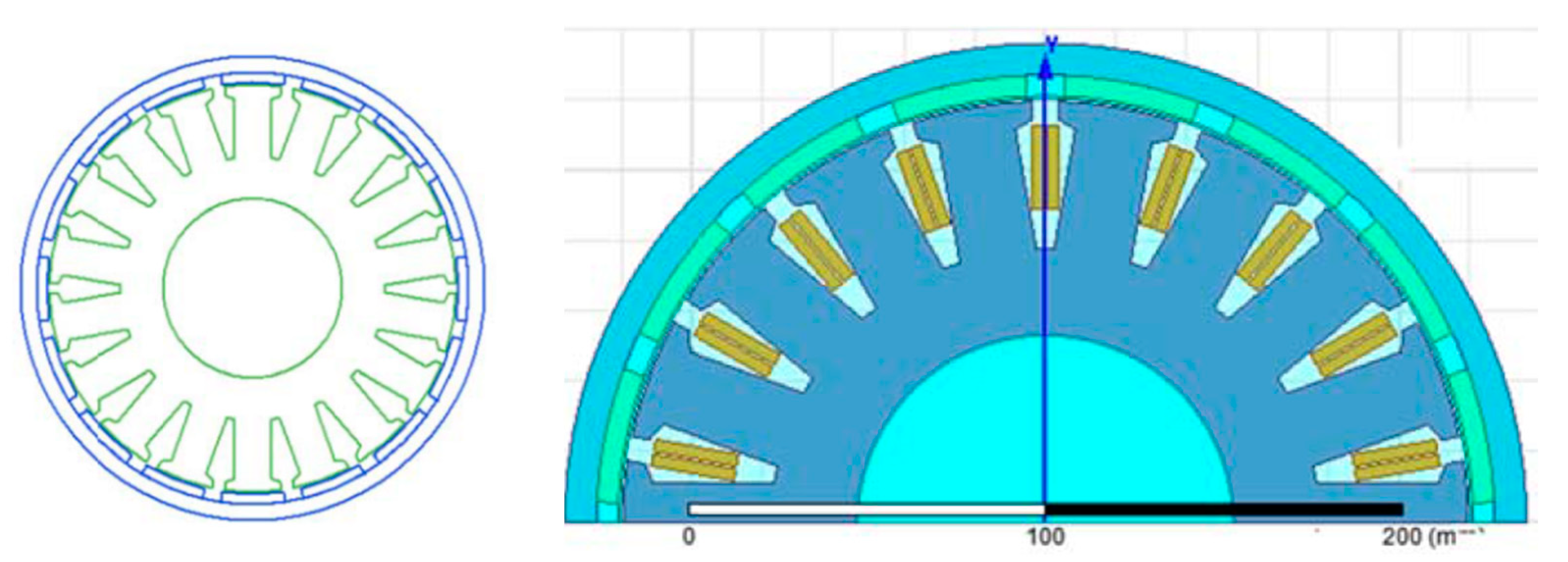
The motor design specification is shown in

Table 1. The main parameters of a permanent magnet synchronous machine (PMSM).

Rated power	10.39 kW	Outer diameter of the stator	234 mm
Rated speed	1039 rpm	Maximum speed	1400 rpm
PM thickness	8 mm	PM material	NdFeB35

. The finite element model is shown in Figure 1.

The correlation coefficient is calculated according to [14], as shown in

Table 2. The constant coefficient of the PM loss under sinusoidal current input.

Coefficient	$\mathit{a} (\mathit{W}/{\mathit{A}}^2)$	$\mathit{b} (\mathit{W}/{\mathit{A}}^2)$	$\mathit{c} (\mathit{W}/\mathit{A})$	$\mathit{d} \left(\mathit{W}\right])$
Value	0.0216	0.0152	−3.836	275.1

.

However, the phase current of stator windings contains rich higher-order time harmonics under PWM input. The PM not only includes sinusoidal PM loss caused by the slot effect and armature reaction of the fundamental current but also includes the eddy current loss caused by the armature reaction of the harmonic current of stator windings, that is, additional PM loss.

In this paper, additional PM losses are analyzed under the entire torque–speed envelope.

3. Constant-Torque Operation Region

According to [15,16,17], the PM loss caused by a harmonic current is proportional to the square of the rotational speed.

As the phase current decreases, the amplitude/fundamental current of the harmonic current increases and the eddy current loss caused by the armature reaction changes a little, so the effect of the phase current can be ignored.

When the amplitude modulation ratio and speed remain constant, the reciprocal relationship between the additional loss and carrier ratio is a quadratic function of one variable.

When the carrier ratio and speed remain unchanged, the additional loss and the amplitude modulation ratio form a quadratic function of one variable. Here, only the amplitude modulation ratio of less than 1 is considered.

Based on the above, the fitting formula of the additional loss under a constant-torque condition can be expressed as

$$\begin{array}{c}{P}_{PM-EL}\left(n,N,M\right)=f\left(N\right)·g\left(M\right)·{\left(\frac{n}{n_R}\right)}^2\\ =\left(a_1\frac{1}{N^2}+b_1\frac{1}{N}+c_1\right)\left(a_2{\left(M-M_0\right)}^2+b_2\left(M-M_0\right)+1\right){\left(\frac{n}{n_R}\right)}^2\end{array}$$

(2)

where $P_{PM-EL}$ is the additional PM loss; $n_R$ is the reference speed; $N$ is the carrier frequency, and its value is $N=f_c/f,$ where $f$ is the fundamental frequency and $f_c$ is the carrier frequency; $M$ is the amplitude modulation ratio; and $a_1$, $b_1$, $c_1$, $a_2$, $b_2$, and $c_2$ are constant coefficients.

In Equation (2), there are five constant coefficients that need to be solved. To solve them accurately and quickly, further simplification is needed.

When the carrier ratio and speed remain constant, the PM loss decreases as the amplitude modulation ratio increases. Since the study considers the case where the amplitude modulation ratio is less than 1, $g\left(M\right)$ can be understood as a correction coefficient based on the amplitude modulation ratio of the variable. With the increase in the amplitude modulation ratio, the correction coefficient decreases and the relation with the pulse width modulation is a quadratic function of one variable.

When the amplitude modulation ratio is set to the reference amplitude modulation ratio, then $g\left(M_0\right)=1$. $f\left(N\right)$ is understood as the fitting formula for the additional PM loss based on the variable carrier ratio, and it is related to the carrier ratio as a quadratic function of one variable. On the basis of the relation, the correction factor based on the variable amplitude modulation ratio and the speed was added.

Through the above simplification, five special working conditions with different carrier ratios and amplitude modulation ratios can be selected, including three carrier ratios and three amplitude modulation ratios, and the time-step finite element analysis of the PM loss can be carried out to calculate the above five constant coefficients.

It should be pointed out that the PM loss analyzed here includes sinusoidal PM loss and additional PM loss. To obtain the additional PM loss, the sinusoidal PM loss should be subtracted first, and the additional PM loss can be obtained through the following equation:

$$P_{PM-EL}=P_{PM-AL}-P_{PM-SL}$$

(3)

where $P_{PM-AL}$ is the total PM loss.

First, the parameters $a_1$, $b_1$, and $c_1$ in $f\left(N\right)$ are determined. Since the amplitude modulation ratio is set as the reference value and $g\left(M\right)=1$, the fitting formula can be simplified as shown in Equation (4).

$$\left[\begin{array}{ccc}\frac{1}{{N_1}^2}& \frac{1}{N_1}& 1\\ \frac{1}{{N_3}^2}& \frac{1}{N_2}& 1\\ \frac{1}{{N_3}^2}& \frac{1}{N_3}& 1\end{array}\right]\left[\begin{array}{c}{a}_1\\ b_1\\ c_1\end{array}\right]=\left[\begin{array}{c}{P}_{PM-EL}\left(n_R,N_1,M_1\right)\\ P_{PM-EL}\left(n_R,N_2,M_2\right)\\ P_{PM-EL}\left(n_R,N_3,M_3\right)\end{array}\right]$$

(4)

where the amplitude modulation ratio $M_1=M_2=M_3$, $g\left(M_3\right)=1$.

Both sides are multiplied by the inverse of the coefficient matrix, which is

$$\left[\begin{array}{c}{a}_1\\ b_1\\ c_1\end{array}\right]={\left[\begin{array}{ccc}\frac{1}{{N_1}^2}& \frac{1}{N_1}& 1\\ \frac{1}{{N_3}^2}& \frac{1}{N_2}& 1\\ \frac{1}{{N_3}^2}& \frac{1}{N_3}& 1\end{array}\right]}^{-1}\left[\begin{array}{c}{P}_{PM-EL}\left(n_R,N_1,M_1\right)\\ P_{PM-EL}\left(n_R,N_2,M_2\right)\\ P_{PM-EL}\left(n_R,N_3,M_3\right)\end{array}\right]$$

(5)

Second, the parameters $a_2$ and $b_2$ in $f\left(N\right)$ are determined.

$$\left[\begin{array}{cc}{\left(M_4-M_0\right)}^2& \left(M_4-M_0\right)\\ {\left(M_5-M_0\right)}^2& \left(M_5-M_0\right)\end{array}\right]\left[\begin{array}{c}{a}_2\\ b_2\end{array}\right]=\left[\begin{array}{c}{P}_{PM-EL}\left(n_R,N_4,M_4\right)\\ P_{PM-EL}\left(n_R,N_5,M_5\right)\end{array}\right]/f\left(N_3\right)$$

(6)

where the carrier ratio $N_3=N_4=N_5$.

On further simplification

$$\left[\begin{array}{c}{a}_2\\ b_2\end{array}\right]={\left[\begin{array}{cc}{\left(M_4-M_0\right)}^2& \left(M_4-M_0\right)\\ {\left(M_5-M_0\right)}^2& \left(M_5-M_0\right)\end{array}\right]}^{-1}\left[\begin{array}{c}{P}_{PM-EL}\left(n_R,N_4,M_4\right)\\ P_{PM-EL}\left(n_R,N_5,M_5\right)\end{array}\right]/f\left(N_3\right)$$

(7)

The reference speed of the prototype is selected as 600 rpm. The prototype works at the rated load, that is, the cross-axis current $i_{qw}$ is 43.1 A and the d-axis current is 0. The coordination of the motor control parameters, carrier ratio, and amplitude modulation ratio is shown in

Table 3. Motor control parameters, carrier ratio, and amplitude modulation ratio.

Motor Control Parameters	1	2	3	4	5
Carrier ratio $\mathrm{N}$	84	54	27	27	27
Amplitude modulation ratio $\mathrm{M}$	0.99	0.99	0.99	0.8	0.6

. The reference speed is lower than the rated speed because the fundamental frequency corresponding to the speed is 80 Hz, which is relatively low. A large finite element step can be set so that the PM loss corresponding to different carrier ratios can be accurately and quickly calculated to improve the calculation efficiency and accuracy.

Through finite element analysis and the calculation method of the above fitting formula, the values of the five constant coefficients in the fitting formula are obtained, as shown in

Table 4. The corresponding constant coefficient of the additional PM loss of the prototype.

Coefficient	${\mathit{a}}_1 \left(\mathit{W}\right])$	${\mathit{b}}_1 \left(\mathit{W}\right])$	${\mathit{c}}_1 \left(\mathit{W}\right])$	${\mathit{a}}_2$	${\mathit{b}}_2$
Value	−3.868 × 103	949.3	9.747	10.31	4.481 × 10−2

.

Figure 2 shows the comparison of additional PM losses under different carrier ratios of the finite element calculation and the fitting calculation. It can be seen that the calculation accuracy of the fitting calculation is high, and it is in good agreement with the finite element results.

Under the condition of higher motor speed and higher carrier ratio, the fitting formula will have a little error. The reasons are as follows: First, the error of calculating the sinusoidal PM loss is inherited, which comes from the interaction of core saturation, inductive eddy current reaction, armature reaction of the alternating axis, and slot effect. Second, in the finite element calculation of high speed and a high carrier ratio compared to the error of the PM loss, due to the high-speed case, the fundamental frequency of the phase current is larger. In the case of high reflection, the stator current harmonic frequency is higher and the corresponding frequency is also higher, so a small step needs to be set up for accurate calculation in order to eliminate the meter and higher harmonic current caused by eddy current loss brought by the error.

Figure 3 shows the comparison of additional PM losses at different amplitude modulation ratios for finite element and fitting calculations. It can be seen that at high speed and a high carrier ratio, there is a small gap between the fitting formula and the finite element calculation results, and the analytical reasons are similar to those mentioned above. When the amplitude modulation is relatively low, this error further increases, because with a decrease in the amplitude modulation ratio, it is difficult for the finite element to calculate the amplitude of the higher harmonic of the phase current, which makes the finite element calculation result small.

4. Constant-Power Operation Region

When a PMSM works under a constant-power condition, due to the direct axis current, compared with the constant-torque condition, the stator phase current and its higher harmonic amplitude change. These changes have a certain regularity, so there is a corresponding rule for the PM loss caused by the armature reaction of the harmonic current. It can be known from [18] that the harmonic amplitude of the stator phase current with the d-axis current is $\frac{{i_q}^2}{{i_d}^2+{i_q}^2}$ times that of the stator phase current without the d-axis current. Therefore, the PM loss caused by the armature reaction of the harmonic current is $\frac{{i_q}^2}{{i_d}^2+{i_q}^2}$ times of the original. The additional PM loss at the constant-power operation region can be expressed by the following formula:

$$\begin{array}{c}{P}_{PM-EL}\left(n,N,M\right)=f\left(N\right)·g\left(M\right)·{\left(\frac{n}{n_R}\right)}^2·\frac{{i_q}^2}{{i_d}^2+{i_q}^2}\\ =\left(a_1\frac{1}{N^2}+b_1\frac{1}{N}+c_1\right)\left(a_2{\left(M-M_0\right)}^2+b_2\left(M-M_0\right)+1\right){\left(\frac{n}{n_R}\right)}^2·\frac{{i_q}^2}{{i_d}^2+{i_q}^2}\end{array}$$

(8)

On the basis of the fitting formula in Equation (2), the additional PM loss in the constant-power region is modified with the alternating and d-axis current as the variable. Therefore, the fitting formula in Equation (2) is a special form of the fitting formula in Equation (8), that is, the formula is the case where $i_d=0$. This is because when the stator winding acts solely on the quadrature axis current, the value of the q-axis current increases and the amplitude of the harmonic current decreases. In general, the q-axis current has little effect on the PM loss, which can be ignored. When the stator winding generates the d-axis current, the change in the harmonic current amplitude is directly related to the q-axis and the d-axis current. The above correction coefficient can be used to obtain a more accurate calculation method of the additional PM loss. The constant coefficient of the fitting formula in Equation (2) is the same as that of the fitting formula in Equation (8). Therefore, the fitting formula in Equation (8) can be determined only by determining the d-axis current and the q-axis current, and there is no need to use the finite element to determine the additional PM loss under special conditions, which can further save the operation time. The fitting formula in Equation (8) takes into account the influence of time harmonics of the stator winding current, but just like the sinusoidal PM loss mentioned above, it ignores the interaction of the q-axis armature reaction, core saturation effect, and slot effect, as well as the influence of the eddy current reaction on the additional PM loss.

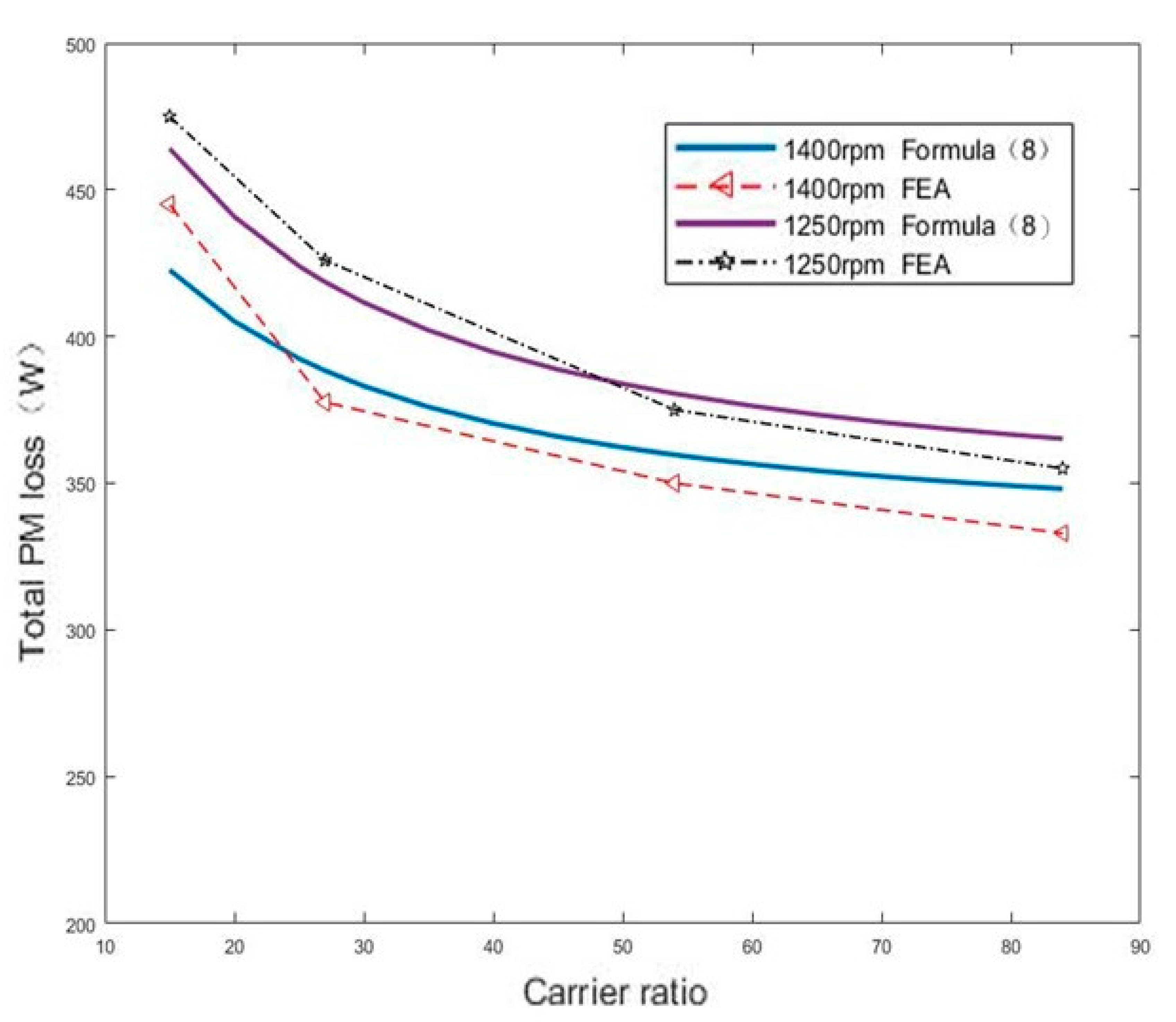
Figure 4 shows the comparison of additional PM losses under different carrier ratios calculated by the finite element method and the fitting formula in Equation (8) at two speeds under constant-power conditions. Smaller errors appear in the calculation results, because the error of the additional PM loss under the constant-power condition is inherited by the fitting formula, that is, the error of the sinusoidal PM loss fitting formula under the constant-power condition and the error of the sinusoidal PM loss fitting formula under the constant-torque condition. However, the error is small. In general, the fitting formula can fit the additional PM loss under the constant-power condition well.

5. Modification in the Full Operational Envelope

The above analysis of PM loss is based on the assumption that the operating temperature of PMs is constant. However, when PM loss leads to a temperature increase in PMs, the PM material demagnetizes and the residual flux decreases. As a result, the amplitude of space harmonic and time harmonic changes in the PM, which affects the generation of PM loss. At the same time, the conductivity of the PM changes with the temperature. The conductivity of the PM decreases with an increase in temperature. There is a direct linear relationship between the PM loss and the conductivity of PM. The lower the conductivity, the lower the PM loss. However, the PMSMs for vehicle applications need to work in a variety of complex and variable conditions, and the temperature of the PM dramatically changes. Therefore, it is necessary to embed the temperature factor into the fitting formula method of PM loss to eliminate the calculation error of PM loss caused by temperature changes.

5.1. The Influence of Temperature on the Remanence of PMs

With the increase in temperature, the magnetic performance loss of a PM includes reversible loss and irreversible loss. When the temperature reaches the Curie temperature, the magnetic performance disappears. The relationship between the residual magnetic flux density of the PM and temperature changes is shown in the formula in Equation (9). The curve of the residual magnetic flux density of the PM with temperature is shown in Figure 5.

$$B_r=B_{r0}\left(1+{\alpha }_1\left(T-T_0\right)+{\alpha }_2{\left(T-T_0\right)}^2\right)0°\mathrm{C}\le T\le 120°\mathrm{C}$$

(9)

where ${\alpha }_1$ and ${\alpha }_2$ are the temperature coefficients of the residual magnetic flux of the permanent magnet, $T_0$ is the reference temperature, and $B_{r0}$ is the residual magnetic flux density when the temperature is $T_0(°\mathrm{C}$).

According to [14], the PM loss caused by the slotting effect is proportional to the square of the residual magnetic flux density of the PM. The PM loss caused by the armature reaction has nothing to do with the residual magnetic flux density of the PM. Therefore, only the coefficients related to the slotting effect in the fast calculation method of PM loss need to be corrected to obtain the following formula:

$$\begin{array}{c}{P}_{PM-SE}\left(n^2,i_d,B_r\right)=\left(c{i}_d\left(\frac{B_r}{B_{r0}}\right)+d{\left(\frac{B_r}{B_{r0}}\right)}^2\right){\left(\frac{n}{n_w}\right)}^2\\ =\left(c{i}_d\left(1+{\alpha }_1\left(T-T_0\right)+{\alpha }_2{\left(T-T_0\right)}^2\right)+d{\left(1+{\alpha }_1\left(T-T_0\right)+{\alpha }_2{\left(T-T_0\right)}^2\right)}^2\right){\left(\frac{n}{n_w}\right)}^2\end{array}$$

(10)

where ${\alpha }_{B_r}$ is the temperature coefficient of the residual magnetic flux of the PM.

Figure 6 shows the relationship between the PM loss caused by the slotting effect and the operating temperature calculated by the fitting formula in Equation (10) and the finite element calculation. The conductivity change caused by temperature change is not considered here, that is, only the influence of temperature change on the residual magnetic flux density is considered. In the finite element analysis, the residual magnetic flux density and coercive force are changed to keep the relative permeability constant. It can be seen from the figure that the difference between the calculation results of the finite element and analytical methods is small; the temperature increases, and the PM loss decreases.

5.2. The Influence of Temperature on the Conductivity of PMs

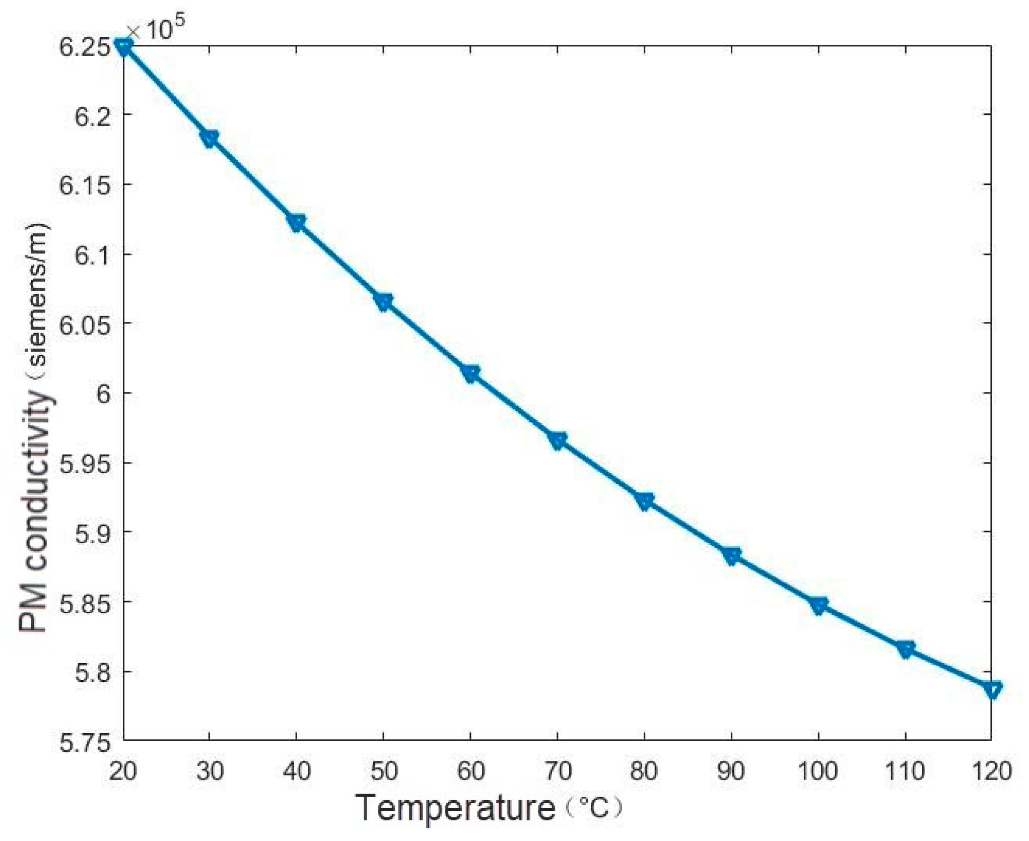
The relationship between the conductivity of NdFeB and the temperature is shown in formula in Equation (11), that is, conductivity is inversely proportional to the quadratic function of temperature. Figure 7 shows the relationship between the conductivity of NdFeB in this paper and temperature:

$${\sigma }_{NTP}={\sigma }_{NTP0}\frac{1}{\left(1+{\beta }_1\left(T-T_0\right)+{\beta }_2{\left(T-T_0\right)}^2\right)}$$

(11)

where ${\sigma }_{NTP0}$ is the conductivity when the temperature is $T_0$ and ${\beta }_1$ and ${\beta }_2$ are the correction coefficients for the conductivity of the PM.

According to [15,16,17], ignoring some of the less influential factors, the entire PM loss is proportional to conductivity. It is assumed that when the temperature changes, the internal resistivity of the PM changes isotropically. The computationally efficient method of PM loss, considering resistance change, can be expressed as

$$\begin{array}{c}{P}_{PM-AL}=\frac{{\sigma }_{NTP}}{{\sigma }_{NTP0}}\left(P_{PM-SL}+P_{PM-EL}\right)\\ =\frac{1}{\left(1+{\beta }_1\left(T-T_0\right)+{\beta }_2{\left(T-T_0\right)}^2\right)}\left(P_{PM-SL}\left(n^2,i_d,B_r\right)+P_{PM-EL}\left(n,N,M\right)\right)\end{array}$$

(12)

where

$$P_{PM-SL}\left(n^2,i_d,B_r\right)=\left(a{i_q}^2+b{i_d}^2+c{i}_d\left(\frac{B_r}{B_{r0}}\right)+d{\left(\frac{B_r}{B_{r0}}\right)}^2\right){\left(\frac{n}{n_w}\right)}^2$$

(13)

Figure 8 shows the relationship between operating temperatures and the results calculated by the fitting formula in Equation (12) and the finite element calculation. Here, the effects of both PM remanence and conductivity changes are considered. Figure 8a shows that when the q-axis current is large, as the temperature increases, a smaller error occurs. The analysis reason is the interaction of the q-axis current armature reaction and the PM remanence change and the saturation of the stator core. Therefore, the fitting formula in Equation (12) can calculate the PM loss at different temperatures.

5.3. Electrical Resistivity Correction Factor

Although two-dimensional FEA can calculate the PM loss relatively accurately and quickly, it cannot consider the effect of the PM end and the influence of PM segmentation. According to [19], based on the idea of an equivalent electric rent, the PM loss has a certain rule between three-dimensional and two-dimensional FEA calculation results, which can be expressed by the width and length of the PM. Assuming that the resistivity of the PM is isotropic, the electrical resistivity correction factor can be expressed as

$$\mathrm{F}=\frac{P_{3D}}{P_{2D}}=\frac{3}{4}\frac{L^2}{w^2+L^2}$$

(14)

where $P_{3D}$ is the PM loss calculated by three-dimensional FEA, $P_{2D}$ is the PM loss calculated by two-dimensional FEA, $L$ is the axial length of the PM, and $w$ is the width of the PM.

However, the above correction factor is only applicable to the correction of the PM loss caused by the armature reaction. When the PM loss caused by the slotting effect is too large, the errors become larger. According to the method proposed by [14], the ratio of the PM loss of the reference speed open-circuit condition can be calculated by 2-D and 3-D FEAs as the correction factor of the PM loss caused by the slotting effect, which can be expressed as follows:

$$\mathsf{\eta }=\frac{P_{PM-SE-3D}}{P_{PM-SE-2D}}$$

(15)

where $P_{PM-SE-2D}$ is the PM loss calculated by 2-D FEA at a reference speed under open-circuit conditions and $P_{PM-SE-3D}$ is the PM loss calculated by 3-D FEA at the reference speed under open-circuit conditions.

The whole PM eddy current fitting formula is fitted by the PM loss value of the PM at a special operating point calculated by two-dimensional FEA. It can be improved by η and F, and a more accurate fitting formula is obtained as follows:

$$P_{PM-AL}=\frac{1}{\left(1+{\beta }_1\left(T-T_0\right)+{\beta }_2{\left(T-T_0\right)}^2\right)}\left(P_{PM-SL}\left(n^2,i_d,B_r,\eta ,F\right)+P_{PM-EL}\left(n,N,M\right)F\right)$$

(16)

where

$$P_{PM-SL}\left(n^2,i_d,B_r,\eta ,F\right)=\left(\left(a{i_q}^2+b{i_d}^2\right)\eta +\left(c{i}_d\left(\frac{B_r}{B_{r0}}\right)+d{\left(\frac{B_r}{B_{r0}}\right)}^2\right)F\right){\left(\frac{n}{n_w}\right)}^2$$

(17)

6. Verification

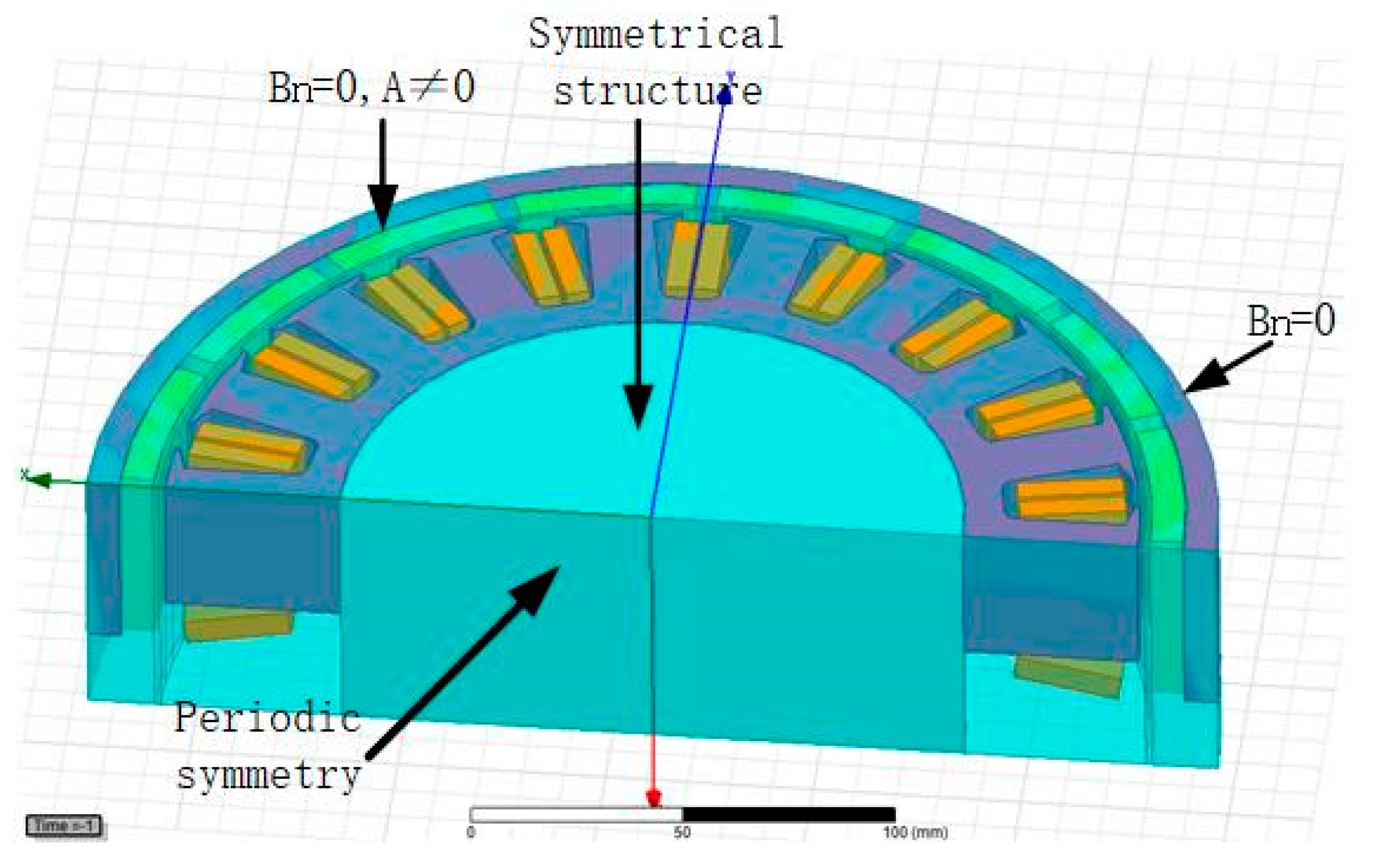
The 3-D FEA model has many element grids, and the mutual matching between the grids is complicated and the calculation cycle long. Therefore, by combining the axial structural symmetry of the motor and the periodic symmetry of the motor radial direction, the 3-D FEA model is simplified, as shown in Figure 9. Figure 10 shows the eddy current density of PMs of a pole in 3-D FEA of the prototype under working conditions (speed is 600 rpm, pulse width modulation ratio is 0.99, and the carrier ratio is 27). The eddy current inside the PM forms a loop at the end of the PM, which can account for the influence of the end effect of the PM on the loss.

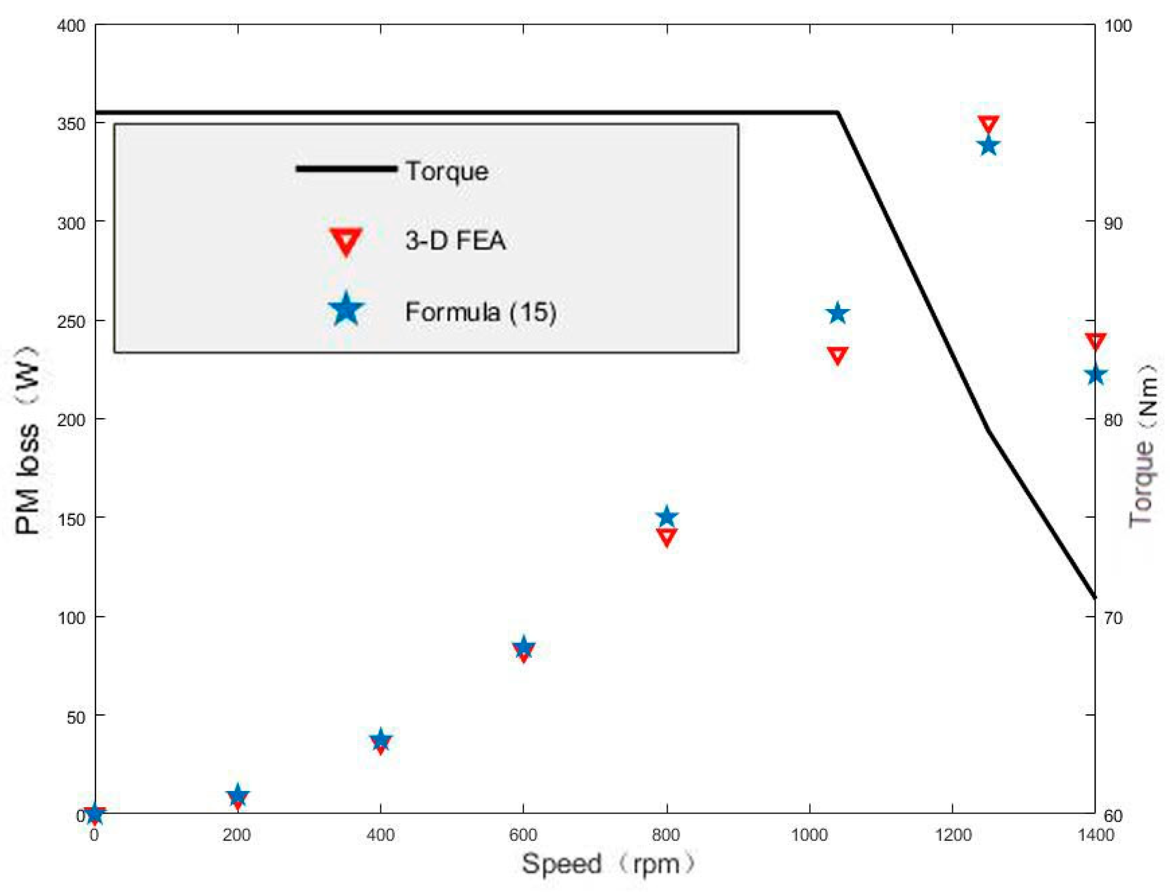
The PM loss at several operating points of the characteristic curve of the rated operating condition is calculated using the fitting formula in Equation (15) and 3-D FEA. Figure 11 shows the comparison of the calculation results of the two methods. In the figure, the carrier ratio and amplitude modulation ratio are kept unchanged at 27 and 0.99, respectively. It can be seen that the predicted value of the fitting formula in Equation (15) is in good agreement with the 3-D FEA results. Smaller errors will inevitably occur, which come from the reaction of induced eddy currents and the end effect of PMs. To eliminate these errors, more finite element working points are needed to correct the fitting formula.

To further verify the practicability of the proposed novel method, another motor was experimentally verified. The parameters of the motor are given in

Table 5. The main parameters of the PMSM.

Rated power	5 kW	Outer diameter of the stator	112 mm
Rated speed	842 rpm	Maximum speed	1050 rpm
PM thickness	6 mm	PM material	YXG-30L

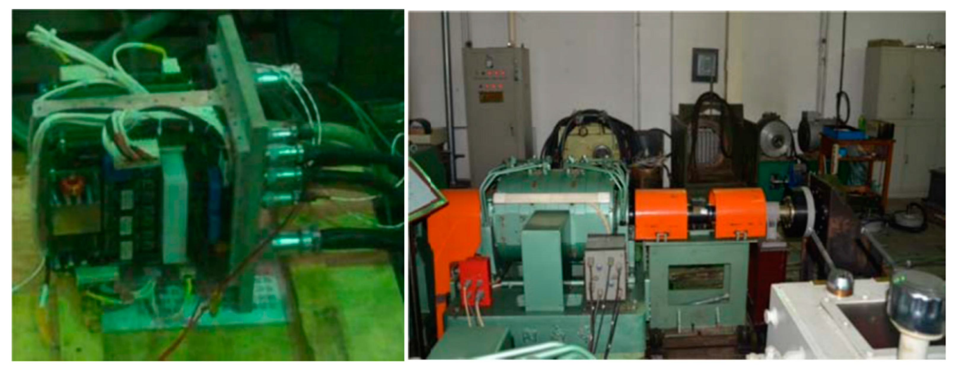
. The motor prototype structure and the finite element model are shown in Figure 12. The prototype stator and the rotor are shown in Figure 13. Figure 14 shows the controller and the experimental bench.

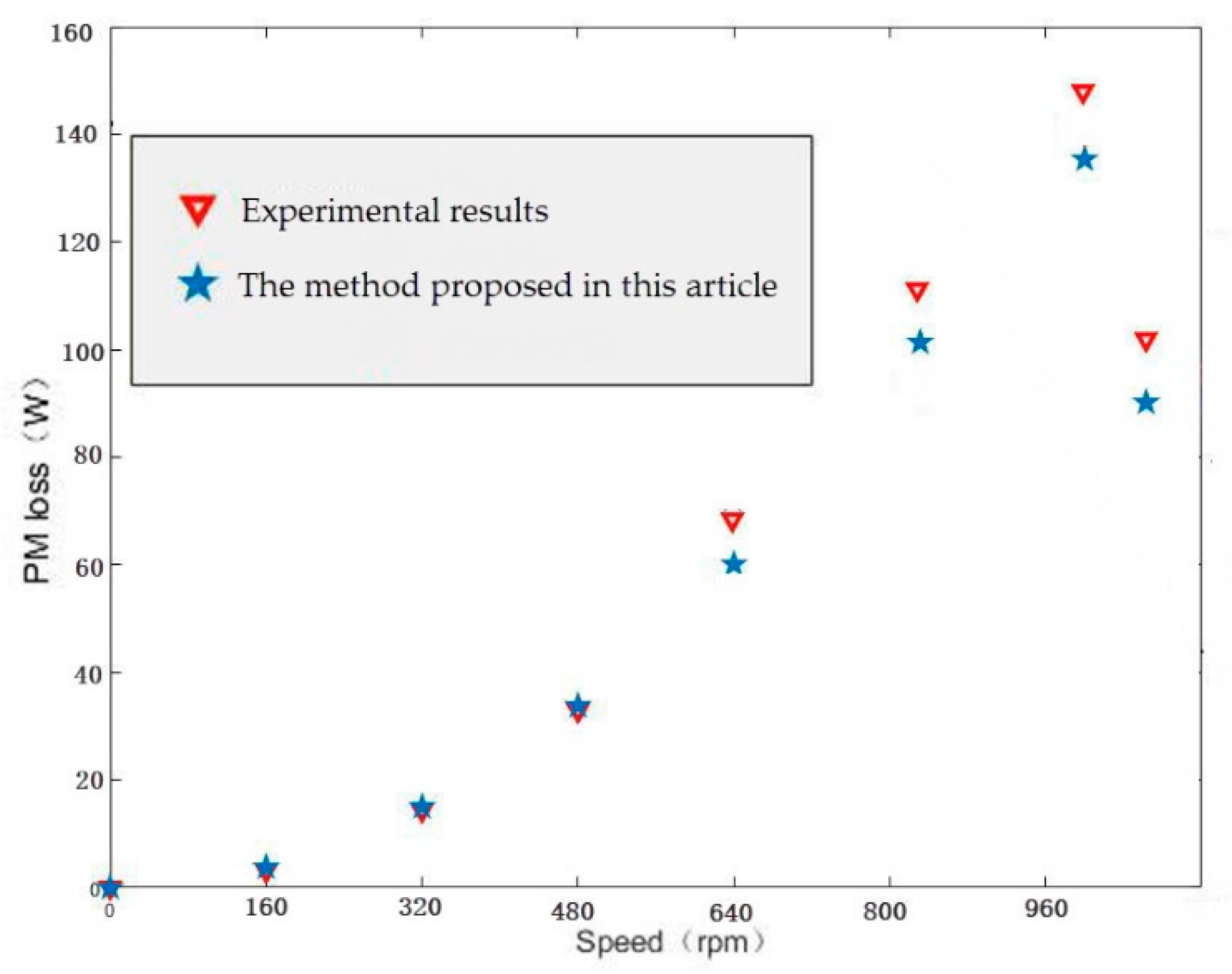
In this study, the separation loss method is adopted, which means that the total loss that is about to be obtained is subtracted from other losses during the operation of the permanent magnet synchronous motor, and then the permanent magnet loss is obtained. The power analyzer is used to test the total input power when the motor is running, and then the torque sensor is connected to the rotor side of the motor to obtain the output power of the motor. The total loss of the motor is the difference between the input power and the output power. The total loss subtracts the copper loss, stator and rotor iron loss, and mechanical loss to obtain the permanent magnet loss. The experimental results and calculation results of the method proposed in this paper are shown in Figure 15.

It can be seen from Figure 15 that the method proposed in this paper is consistent with the experimental data. The error is because the loss separation method inherits the errors of other loss measurements (stator and rotor iron loss, winding copper loss, mechanical loss, etc.), resulting in large PM losses.

To eliminate the error of the separation loss method, in recent years, scholars have proposed the direct measurement method. The temperature sensor is used to accurately predict the temperature change of the permanent magnet, and then the eddy current loss of the permanent magnet is obtained according to the temperature field model of the motor. The arrangement of the temperature sensor in the rotor is restricted, and at the same time, it will have an impact on the structure of the rotor and the electromagnetic field of the motor. The implementation of this method is more difficult, and it is one of the directions of permanent magnet loss research in the future.

In general, the proposed fitting formula can predict the PM loss relatively efficiently, while taking into account the influence of temperature factors and time harmonics. This method is effectively embedded in the design of the PMSM, improves the design efficiency, and shortens the design cycle.

7. Conclusions

This paper proposes a computationally efficient approach to estimate the PM loss of the PMSM’s full operational envelope. The method outlined in this paper builds on the work of previous scholars on PM loss mapping. For the first time, a computationally efficient method for the additional PM loss in the full operational envelope range with the carrier ratio, pulse width modulation ratio, d-axis current, q-axis current, and speed is proposed, and the temperature factor is considered. The proposed methodology is compared with the results of a single three-dimensional finite element analysis of each operating point, which shows the close correlation of the entire operational envelope. Two motors and an experiment illustrating the use and fidelity of the proposed technique have been given. These include rotor construction with differing levels of segmentations for the analyzed machine exemplar.