Time-Continuous Real-Time Trajectory Generation for Safe Autonomous Flight of a Quadrotor in Unknown Environment

Abstract

In this paper, we present an efficient global and local replanning method for a quadrotor to complete a flight mission in a cluttered and unmapped environment. A minimum-snap global path planner generates a global trajectory that comprises some waypoints in a cluttered environment. When facing unexpected obstacles, our method modifies the global trajectory using geometrical planning and closed-form formulation for an analytical solution with 9th-order polynomial. The proposed method provides an analytical solution, not a numerical one, and it is computationally efficient without falling into a local minima problem. In a simulation, we show that the proposed method can fly a quadrotor faster than the numerical method in a cluttered environment. Furthermore, we show in experiments that the proposed method can provide safer and faster trajectory generation than the numerical method in a real environment.

1. Introduction

Small UAVs(unmanned aerial vehicles) have a limitation in their payload, and can carry only a small computer. This means that heavy and complex computation is difficult to operate on a UAV’s on-board computer. With limited computation power, it is difficult to prevent collisions caused by the sudden appearance of obstacles in front of the small UAV during an autonomous flight [1]. A UAV has to replan the global trajectory in order to fly in an unmapped and cluttered environment. In this paper, we present an efficient method of replanning the quadrotor’s global trajectory for safe flight.

Thanks to the differential flatness property [2], the quadrotor’s desired motor speed and state can be represented as a 3D coordinate and orientation of a quadrotor. If the quadrotor has the trajectory, it can compute the desired motor speed and state from the differential flatness. Iteration-based optimization methods are widely used for generating global trajectory, such as the unconstrained Quadratic Programming (QP) method [3], which shows a fast computation speed and provides a collision-free trajectory using a visibility graph [4]. The global trajectory is computed before the quadrotor’s flight using the previously mapped environment to generate the global trajectory. When a quadrotor faces an obstacle, it needs to replan its global trajectory. There are advanced techniques for replanning to prevent collision and ensure successful safe flight. In the reactive method [5], the quadrotor does not build any map during the flight  [6,7]. It depends on a camera sensor attached on the front of the robot. When an object is detected in the camera by the detection or classifying algorithm, the replanning algorithm commands the robot to move to the right or left rather than continuing straight. This method is high-speed, but when too many objects are detected, such replanning algorithms tend to fail. Sampling-based methods such as RRT (rapidly exploring random tree)  [8] build a road map from sampling free space and searches the graph map space by computing the edge cost and heuristic functions [9]. However, the RRT path is non-smooth in general, and it often does not satisfy the quadrotor’s dynamic constraint. The smoothing step is necessary to ensure kinematic and dynamic feasibility  [3]. This method builds a visibility graph to construct a non-smooth path, but it takes too much time to execute in real-time on an on-board computer.

Another method is the trajectory optimization method, which uses two kinds of cost function to make a collision-free path  [10]. One is a smoothing function, and the other is a collision avoidance function [11]. To minimize the sum of the cost function, researchers have used optimizations such as gradient-descent methods [12] or Gauss–Newton, by computing the gradient or Jacobian of each cost function. By setting proper constraints on polynomials (e.g., velocity and kinematic constraints), the trajectory can satisfy dynamic feasibility. This method can generate a non-collision trajectory in a cluttered environment. Optimization needs to find the best solution for the whole function, but a local minimum smaller than the neighboring values does not guarantee the optimal solution for the whole function [13]. When local minima occur, the trajectory hits an obstacle or induces infeasible movement, causing a dangerous situation for humans and robots.

In this work, we address an analytical method to guarantee a safe trajectory. The analytical method is free from local minima problems, which means a safe replanning trajectory can be generated. The proposed method is also much faster than numerical methods because it can omit the iteration process [14]. Therefore, a quadrotor can fly faster, as an on-board computer can compute solutions in real-time. Moreover, we combine all systems (e.g., localization, mapping, control, and vision) for quadrotor autonomous flight [15]. Even though trajectory generation completes, if other functions do not work as fast or correctly, the quadrotor cannot succeed in its mission. We show the effectiveness of our method in simulation and experiments using Robot Operating System (ROS) programming [16] to connect communication between different devices such as a flight controller [17] and an on-board computer.

The rest of this paper is composed as follows. Section 2 presents how to generate the global and local trajectory of a quadrotor. Section 3 shows the simulation and the real experimental test results, and finally Section 4 provides a conclusion and discussion.

2. Trajectory Generation

2.1. Global Trajectory Generation

As quadrotors have differential flatness property [2], a 3D coordinate ($x,y,z$) trajectory (except for the yaw angle ($\psi$)) of the quadrotor is generated, since the yaw angle is responsible for the camera’s direction. A yaw angle trajectory is generated independently. The whole trajectory is divided into a series of segments indicated by waypoints. Each of these segments has a polynomial-based trajectory from its starting waypoint to an ending waypoint. This relationship can be described by the Nth-order polynomial ($P\left(t\right)$) as shown below. However, this function only covers the trajectory of one axis. Thus, in order to fully represent a 3D trajectory, the formula must be used on all axes.

$$P\left(t\right)=a_0+a_{1}t+a_2{t}^2+a_3{t}^3+\cdots +a_N{t}^N$$

(1)

$$\mathbf{p}={\left[a_0,a_1,a_2,\cdots ,a_N\right]}^{⊺}$$

(2)

where vector $\mathbf{p}(\in {\mathbb{R}}^{N\times 1})$ are polynomial coefficients. Due to the differential flatness property of quadrotors, the desired motor speed of the quadrotor is represented by the fourth derivative of its position. By minimizing snap, an optimal trajectory can be obtained. The equation is as follows.

$$argmi{n}_p{\int }_0^T{∥\frac{d^{4}P\left(t\right))}{d{t}^4}∥}^{2}dt$$

(3)

$$\mathbf{A}\mathbf{p}=\mathbf{d}$$

(4)

where T is the end time of the trajectory segment, and $\mathbf{A}(\in {\mathbb{R}}^{N\times N})$ is a mapping matrix from polynomial coefficients to the trajectory constraints at the start time or end time. Vector $\mathbf{d}$ represents trajectory constraints of position (p), velocity (v), acceleration (a), jerk (j), and snap (s). The m-th segment of d is represented as $d_m$.

$${\mathbf{d}}_{\mathbf{m}}={\left[p_m,v_m,a_m,j_m,s_m,p_{m+1},v_{m+1},a_{m+1},j_{m+1},s_{m+1}\right]}^{⊺}$$

(5)

where $p_m,v_m,a_m,j_m,s_m$ is the m-th segment of position, velocity, acceleration, jerk, and snap. As seen in Equation (5), we use constraints up to snap, meaning that one segment polynomial has 10 constraints where 5 constraints are located at the start point and the remaining 5 are located at an endpoint, so we should use a 9th-order polynomial as a trajectory.

To extend the equation, we can rewrite (3) as follows:

$${\int }_0^T{∥\frac{d^{4}P\left(t\right)}{d{t}^4}∥}^{2}dt={\mathbf{p}}^{⊺}\mathbf{Qp}$$

(6)

where $\mathbf{Q}$ is the mapping matrix from coefficient to the integral of the squared norm of the fourth derivative. Again, the $\mathbf{Q}$ matrix is as follows when the polynomial is of 9th order.

$$\mathbf{Q}=\left[\begin{array}{ccccccccc}0& 0& 0& 0& 0& 0& 0& 0& 0\\ & & & & ⋮& & & & & \\ 0& 0& 0& 0& {24}^{2}T& \frac{24·120}{2}{T}^2& & \cdots & & \\ 0& 0& 0& 0& \frac{24·120}{2}{T}^2& \frac{120·120}{3}{T}^3& & \cdots & & \\ & & & & ⋮& & & & & \\ & & & \cdots & & & & \frac{1680·3024}{10}{T}^{10}& \frac{{3024}^2}{3}{T}^3\end{array}\right]$$

(7)

where the matrix dimension of $\mathbf{Q}$ is 10 × 10. Using quadratic programming, the quadratic Equation (6), otherwise known as the cost function, can be minimized in order to obtain an optimal trajectory. However, the iteration process is required for optimization, which can be a heavy task due to the number of parameters needed to calculate the polynomial coefficients; thus, this method is not very efficient when the quadrotor has too many waypoints. To solve this problem, unconstrained quadratic programming was proposed by Richter, Bry, and Roy [3]. Unconstrained quadratic programming solves the optimal trajectory directly without iteration, so the computation time can be reduced. They divided constraints into two kinds: fixed derivatives ${\mathbf{d}}_{\mathbf{F}}$ and free derivatives ${\mathbf{d}}_{\mathbf{P}}$. ${\mathbf{d}}_{\mathbf{F}}$ are waypoint position and constraints for continuity. ${\mathbf{d}}_{\mathbf{P}}$ are the free variables velocity and acceleration at the waypoint. Especially in the global trajectory domain, each waypoint is a fixed derivative. All derivatives of the start point and endpoint are fixed to 0.

$$\mathbf{M}\mathbf{d}=\left[\begin{array}{c}{\mathbf{d}}_{\mathbf{F}}\\ {\mathbf{d}}_{\mathbf{P}}\end{array}\right]$$

(8)

where $\mathbf{M}(\in {\mathbb{R}}^{n\times n})$ is the mapping matrix used to convert the trajectory vector d into a vector with fixed derivatives (${\mathbf{d}}_{\mathbf{F}}$) and free variables (${\mathbf{d}}_{\mathbf{P}}$). $\mathbf{M}$ and ${\mathbf{d}}_{\mathbf{F}}$, ${\mathbf{d}}_{\mathbf{P}}$ vectors are not fixed because the number of waypoints decides its size. However, the principle is the same. Combining Equations (4) and (8) yields the next equation.

$$\mathbf{p}={\mathbf{A}}^{-\mathbf{1}}{\mathbf{M}}^{-\mathbf{1}}\left[\begin{array}{c}{\mathbf{d}}_{\mathbf{F}}\\ {\mathbf{d}}_{\mathbf{P}}\end{array}\right]$$

(9)

Inserting Equation (9) into Equation (6), the following equation is yielded. Now the optimization argument is not the coefficient $\mathbf{p}$ but the free derivatives ${\mathbf{d}}_{\mathbf{P}}$. The number of optimization parameters is also reduced.

$$\mathbf{J}={\left[\begin{array}{c}{\mathbf{d}}_{\mathbf{F}}\\ {\mathbf{d}}_{\mathbf{P}}\end{array}\right]}^{⊺}\underset{\mathbf{R}}{\underbrace{{\mathbf{M}}^{-⊺}{\mathbf{A}}^{-⊺}{\mathbf{QA}}^{-\mathbf{1}}{\mathbf{M}}^{-\mathbf{1}}}}\left[\begin{array}{c}{\mathbf{d}}_{\mathbf{F}}\\ {\mathbf{d}}_{\mathbf{P}}\end{array}\right]=\left[\begin{array}{c}{\mathbf{d}}_{\mathbf{F}}\\ {\mathbf{d}}_{\mathbf{P}}\end{array}\right]\left[\begin{array}{cc}{\mathbf{R}}_{\mathbf{FF}}& {\mathbf{R}}_{\mathbf{FP}}\\ {\mathbf{R}}_{\mathbf{PF}}& {\mathbf{R}}_{\mathbf{PP}}\end{array}\right]\left[\begin{array}{c}{\mathbf{d}}_{\mathbf{F}}\\ {\mathbf{d}}_{\mathbf{P}}\end{array}\right]$$

(10)

where $\mathbf{J}$ is the cost function.

$$\mathbf{J}={\mathbf{d}}_{\mathbf{F}}^{⊺}{\mathbf{R}}_{\mathbf{FF}}{\mathbf{d}}_{\mathbf{F}}+{\mathbf{d}}_{\mathbf{F}}^{⊺}{\mathbf{R}}_{\mathbf{FP}}{\mathbf{d}}_{\mathbf{P}}+{\mathbf{d}}_{\mathbf{P}}^{⊺}{\mathbf{R}}_{\mathbf{PF}}{\mathbf{d}}_{\mathbf{P}}+{\mathbf{d}}_{\mathbf{P}}^{⊺}{\mathbf{R}}_{\mathbf{PP}}{\mathbf{d}}_{\mathbf{P}}$$

(11)

Differentiating J by free derivatives yields the following equation.

$$\frac{\partial \mathbf{J}}{\partial {\mathbf{d}}_{\mathbf{P}}}=2{\mathbf{d}}_{\mathbf{F}}^{⊺}{\mathbf{R}}_{\mathbf{FF}}+2{\mathbf{d}}_{\mathbf{P}}^{⊺}{\mathbf{R}}_{\mathbf{PF}}$$

(12)

After equating Equation (12) to zero, the optimal vector ${\mathbf{d}}_{\mathbf{P}}^{*}$ is obtained.

$${\mathbf{d}}_{\mathbf{P}}^{*}=-{\mathbf{R}}_{\mathbf{PP}}^{-\mathbf{1}}{\mathbf{R}}_{\mathbf{FP}}^{⊺}{\mathbf{d}}_{\mathbf{F}}$$

(13)

By substituting the optimal vector ${\mathbf{d}}_{\mathbf{P}}^{*}$ into Equation (9), the optimal coefficients of the vector are obtained, and finally, the trajectory generation is complete. We allocate the segment time along the distance ratio to keep as constant a velocity as possible because we want a safe and stable quadrotor flight. This means that matrices $\mathbf{A}$ and $\mathbf{Q}$ are computed before flight once the waypoints are determined. After the global trajectory is computed, the quadrotor will fly while following the global trajectory.

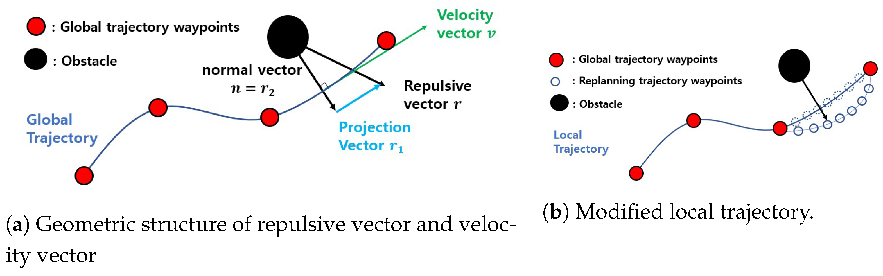
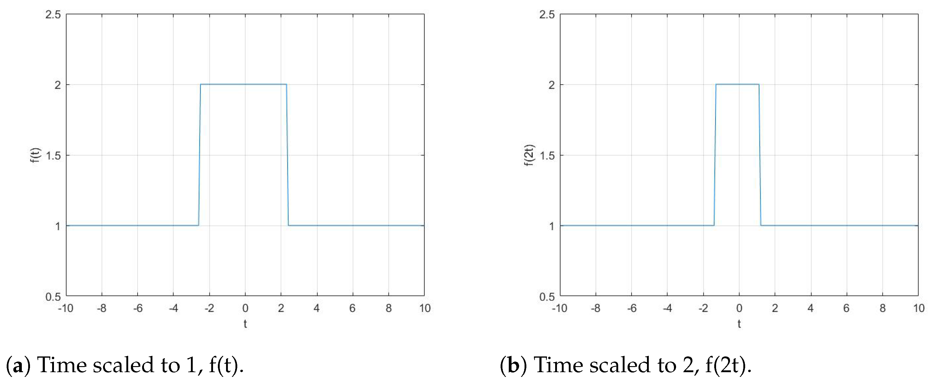
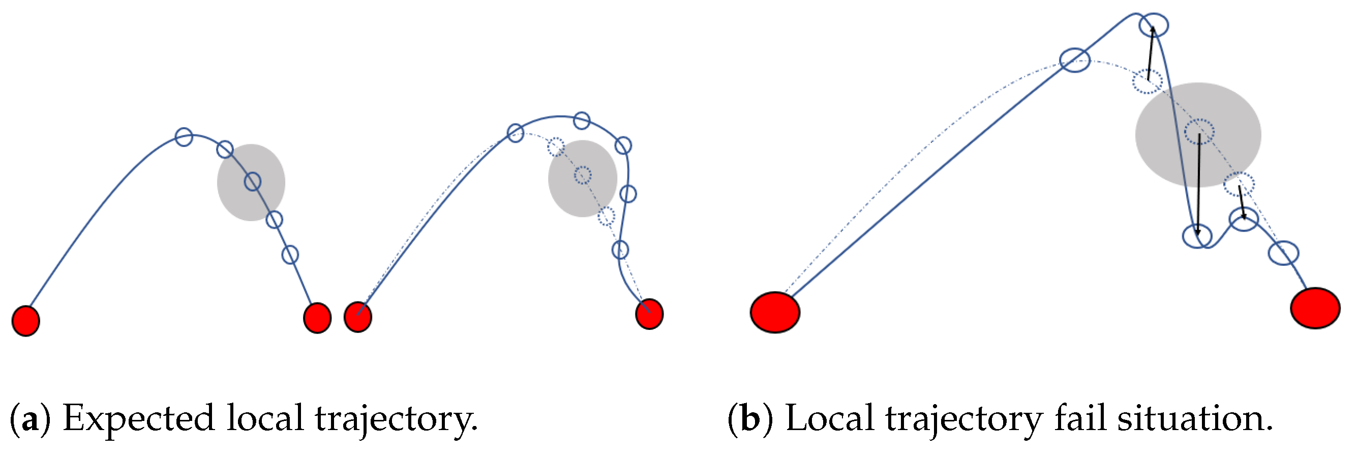
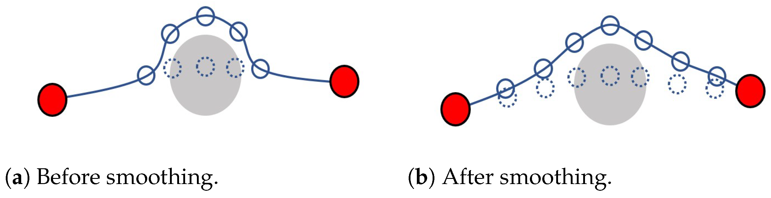
2.2. Closed-Form Local Trajectory Replanning

Instead of an optimization method that computes solutions numerically, we devised a novel method that computes all at once. It solves the local trajectory analytically or geometrically. We use the geometrical information of a map that is built through an occupancy grid [18]. The map has distance and gradient information, so we use gradient values as a repulsive vector ($\mathbf{r}$). When the global trajectory is near the object or in the distance, it repulses the trajectory to avoid collision. We use vector projection (${\mathbf{r}}_{\mathbf{1}}$) and rejection (${\mathbf{r}}_{\mathbf{2}}$) to repulse the trajectory with repulsive vector and velocity vector (v) of the global trajectory as shown in Figure 1a. The velocity vector v is calculated via the first derivative of the trajectory. Mainly, we use the normal vector of the repulsive vector $\mathbf{n}$ to push the global trajectory. The projection and rejection equations are as follows in Equations (14) and (15).

$${\mathbf{r}}_{\mathbf{1}}=\frac{\mathbf{v}·\mathbf{r}}{{∥\mathbf{v}∥}^{\mathbf{2}}}\mathbf{v}$$

(14)

$${\mathbf{r}}_{\mathbf{2}}=r-r_1$$

(15)

We divide the global trajectory into small pieces and modify the waypoints as shown in Figure 1b. The normal vector pushes the global trajectory and modifies it, then a new local trajectory is generated. Now we will show the formulation method that we use for the new local trajectory. If the new waypoint is fixed, we use the non-constrained quadratic programming introduced in Equation (3). By setting some waypoints in fixed derivatives, we can again compute the minimum-snap trajectory. The difference with the global trajectory is as follows.

First, we set the start point and endpoint derivatives; however, as opposed to previously, we do not set them to zero. Instead, we set them at some values for continuity with the current state and global trajectory. Start derivatives are set as the last local trajectory derivatives calculated at the same waypoint. End derivatives are the same values as the global trajectory waypoint.

Second, the segmentation time in the local trajectory is uniform between all waypoints. Because we divide the global trajectory into constant segment times, we can set the time allocation uniformly. Moreover, we use a time scaling factor such that all-time allocation is normalized to 1. An example of time scaling is described in Figure 2. We can represent one function in a different form. Similarly, we can apply time scaling to trajectory generation. If the time scale is applied, derivatives such as velocity must be defined again as in Equations (17) and (18) when the time scaling factor is s and $T=s\times t$.

$$P_1\left(T\right)T\in \left[0,s\right]$$

(16)

$$P_2\left(t\right)=P_2\left(\frac{1}{s}T\right)T\in \left[0,1\right]$$

(17)

$$P_1^{\prime }\left(T\right)=P_2^{\prime }\left(\frac{1}{s}T\right)·\frac{1}{s}=P_2^{\prime }\left(t\right)·\frac{1}{s}$$

(18)

$${\int }_0^s{∥\frac{d^4{P}_1\left(T\right)}{d{T}^4}∥}^{2}dT={\int }_0^1{∥\frac{d^4{P}_2\left(t\right)}{d{t}^4}·\frac{1}{s^4}·dt∥}^{2}s·dt={\int }_0^1{∥\frac{d^4{P}_2\left(t\right)}{d{t}^4}∥}^{2}dt·{\left(\frac{1}{s}\right)}^7$$

(19)

where $P_1$ and $P_2$ are 9th-order polynomial trajectory functions. The time-scaled minimum snap cost, which is the least square of the fourth derivative, is equal to the original cost divided by the scaling factor to the power of seven, as we see in Equation (19). Now we can write the quadratic form as follows.

$${\int }_0^s{∥\frac{d^4{P}_1\left(T\right)}{d{T}^4}∥}^{2}dT={\mathbf{c}}_{\mathbf{1}}^{⊺}\mathbf{Q}\left(T\right){\mathbf{c}}_{\mathbf{1}}$$

(20)

$${\int }_0^1{∥\frac{d^4{P}_2\left(t\right)}{d{t}^4}∥}^{2}dt={\mathbf{c}}_{\mathbf{2}}^{⊺}\mathbf{Q}\left(1\right){\mathbf{c}}_{\mathbf{2}}$$

(21)

$${\mathbf{c}}_{\mathbf{1}}^{⊺}\mathbf{Q}\left(T\right){\mathbf{c}}_{\mathbf{1}}={\left(\frac{1}{s}\right)}^7{\mathbf{c}}_{\mathbf{2}}^T\mathbf{Q}\left(1\right){\mathbf{c}}_{\mathbf{2}}$$

(22)

where ${\mathbf{c}}_{\mathbf{1}}(\in {\mathbb{R}}^{10\times 1})$ and ${\mathbf{c}}_{\mathbf{2}}(\in {\mathbb{R}}^{10\times 1})$ are the coefficient vectors of each polynomial and $\mathbf{Q}$(T), $\mathbf{Q}$(1) are the mapping matrices to convert to the quadratic form. You can see that the segment time T of $\mathbf{Q}$(T) is now replaced by 1 in $\mathbf{Q}$(1). As Equations (20) and (21) show, the relationship between the original quadratic equation and scaled quadratic Equation (22) is proportional to ${\left(\frac{1}{s}\right)}^7$. Now we can write $\mathbf{Q}$(1) matrix as follows.

$$\mathbf{Q}\left(1\right)=\left[\begin{array}{cccccccccc}0& 0& 0& 0& 0& 0& 0& 0& 0& 0\\ & & & & ⋮& & & & & \\ 0& 0& 0& 0& {24}^2& \frac{24·120}{2}& & \cdots & & \\ 0& 0& 0& 0& \frac{24·120}{2}& \frac{120·120}{3}& & \cdots & & \\ & & & & ⋮& & & & & \\ & & & & \cdots & & & & \frac{1680·3024}{10}& \frac{{3024}^2}{11}\end{array}\right]$$

(23)

In this form we are substituting 1 as T in (7). Similarly, matrix $\mathbf{A}$ in (4) is replaced by $\mathbf{A}$(1) by substituting 1 for T.

$$\mathbf{A}\left(1\right)=\left[\begin{array}{cccccccccc}1& 0& 0& 0& 0& 0& 0& 0& 0& 0\\ 0& 1& 0& 0& 0& 0& 0& 0& 0& 0\\ 0& 0& 2& 0& 0& 0& 0& 0& 0& 0\\ 0& 0& 0& 6& 0& 0& 0& 0& 0& 0\\ 0& 0& 0& 0& 24& 0& 0& 0& 0& 0\\ 1& 1& 1& 1& 1& 1& 1& 1& 1& 1\\ 0& 1& 2& 3& 4& 5& 6& 7& 8& 9\\ & & & & ⋮& & & & & \\ 0& 0& 0& 24& 120& & \cdots & & \end{array}\right]$$

(24)

We simplified the $\mathbf{Q}$ and $\mathbf{A}$ matrices and continually used them to replan the local trajectory. This approach can reduce computation complexity. After computing the polynomial coefficient of the local trajectory that is scaled to 1, we restore the trajectory’s real value. Velocity and acceleration are obtained by multiplying by a scale factor, as in  Equation (18). This closed-form method has some merits against the optimization-based numerical method. First, it can solve every case after the waypoints are obtained. As can be seen in Equation (25), the form of the cost function is positive semi-definite.

$$\mathbf{J}={\int }_0^1{∥\frac{d^{4}p\left(t\right)}{d{t}^4}∥}^{2}dT={\mathbf{c}}^{⊺}\mathbf{Qc}={\left[\begin{array}{c}{\mathbf{d}}_{\mathbf{F}}\\ {\mathbf{d}}_{\mathbf{P}}\end{array}\right]}^{⊺}{\mathbf{M}}^{-⊺}{\mathbf{A}}^{-⊺}{\mathbf{QA}}^{-\mathbf{1}}{\mathbf{M}}^{-\mathbf{1}}\left[\begin{array}{c}{\mathbf{d}}_{\mathbf{F}}\\ {\mathbf{d}}_{\mathbf{P}}\end{array}\right]\ge 0$$

(25)

For example, if a hessian matrix is positive semi-definite for any x, $f\left(x\right)$ is convex. We can now see that this closed form is also convex. So, the analytical solution we can obtain by differentiation as in Equation (13) is the global minimum. The second merit is that this method can compute much faster. The fast and simple process allows the quadrotor to navigate a complicated environment where the onboard computer computes the local trajectory. Moreover, fast computation enables the quadrotor to fly faster because the computer can react to objects or obstacles quickly. As shown in Figure 3a, we expect a safe and non-collision local trajectory that avoids obstacles.

If the waypoints were calculated only by gradient information, then the local trajectory could fail, as shown in Figure 3b. Thus, to correct this issue, an Algorithm 1 was created to prevent the failure of the trajectory. If the angle between normal vectors of successive waypoints is over ${90}^{\circ }$ degrees, we reverse the post-normal vector direction.

We realized that when the velocity of navigation is faster, the tracking error is higher. Because the object generates gradient fields only around itself, the local trajectory can be formed steeply. This steep trajectory induces trajectory error, and this could cause the quadrotor to fail to navigate, depending on the scale of the error.To prevent this, we add a smoothing process. The process is shown in Figure 4. Moreover, we considered a dynamically feasible trajectory. From Newton’s equation and differential flatness property, the quadrotor’s thrust ($u_1$) value can be expressed as follows.

$$u_1=m\sqrt{{\ddot{\sigma }}_1^2+{\ddot{\sigma }}_2^2+{({\ddot{\sigma }}_3^2+g)}^2}$$

(26)

where ${\ddot{\sigma }}_1,{\ddot{\sigma }}_2,{\ddot{\sigma }}_3$ are the acceleration of the quadrotor in the x, y, and z axes.

$$u_1\le u_{max}$$

(27)

$$u_{max}=4·k_F·{\Omega }_{max}^2$$

(28)

where $u_{max}$ is the maximum thrust, ${\Omega }_{max}$ is the maximum rotor speed, and $k_F$ is a thrust coefficient. The relationship is in quadratic form.If the $u_1$ is greater than the maximum input, we add some waypoints to slow down the acceleration. The required force (the input of the quadrotor) can be reduced by adding smoothing waypoints, as shown in Figure 5.

In summary, the local trajectory is safe from a collision and has real-time computation speed. Because the trajectory uses a polynomial, it satisfies kinematic constraints by differentiating the polynomial and guaranteeing continuity. Additionally, the trajectory satisfies dynamic constraints by applying a differential flatness property.

Algorithm 1 Replanning waypoints.

1: $\mathbf{n}\mathbf{1}$ and $\mathbf{n}\mathbf{2}$ are normal vectors of waypoints. 2: $\theta$ is the angle between the normal vectors of successive waypoints. 3: $cos\theta =\frac{{\mathbf{n}}_{\mathbf{1}}·{\mathbf{n}}_{\mathbf{2}}}{∥{\mathbf{n}}_{\mathbf{1}}∥∥{\mathbf{n}}_{\mathbf{2}}∥}$ 4: if$\theta >\frac{\pi }{2}$then 5:     ${\mathbf{n}}_{\mathbf{2}}=-{\mathbf{n}}_{\mathbf{1}}$ 6: end if

3. Results

3.1. Simulation

Simulation of the experiments was done using RotorS and ROS (Robot Operating System) in Ubuntu 18.04 [16]. RotorS composes multirotor components by ROS URDF file and shows it in a Gazebo environment. It uses an ODE(Ordinary Differential Equation) physics engine to describe the motion of the multirotor. Rotors have a geometric controller [19] inside, which controls position and attitude. It is possible to get ground-truth data or sensor data with noise and covariance of position and attitude.

As the testing environment, we made a cluttered environment in Gazebo which included some box objects for the obstacles, as shown in Figure 6. A collision occurred when the quadrotor flew into an object and resulted in failure. We were also able to change the environment to any desired preference. However, we determined that this default map was sufficient for testing our algorithm.

In ROS, Usenko’s visualization interface [20] for Rviz was used. For example, “Marker” or “MarkerArray” of “Visualization” was used to show the global trajectory, local trajectory, and 3D occupancy grid, as shown in Figure 7.

While flying in a cluttered environment with a global trajectory, the quadrotor will sense the objects with the camera and depth sensor. A depth camera is used to build a 3D map of the surroundings.From the depth image data, the distance can be measured from the camera to the object.

The algorithm was tested in the simulation by having the quadrotor fly at various speeds and trajectories. The path planning of a straight line global trajectory at speed 2 m/s is shown in Figure 8a–c and Figure 9a. The path planning of the curved global trajectory at a speed of 3 m/s is shown in Figure 8d–f and Figure 9b. The path planning of the curved global trajectory at a speed of 4 m/s is shown in Figure 8g–i and Figure 9c. With our method, we could fly the quadrotor at a speed of up to 4 m/s. The results of this experiment demonstrate that this algorithm is faster than other methods. This is due to the optimized computation of the trajectory performed in this method. The mean computation time is shown in

Table 1. Mean computation time.

Speed (m/s)	Number of Points	Mean Computation Time
2	5	11 × ${10}^{-6}$ s
3	10	17 × ${10}^{-6}$ s
4	20	35 × ${10}^{-6}$ s

. Each point can be seen to be generated between 17.5 × ${10}^{-6}$ s to 2.5 × ${10}^{-6}$ s. There are some parameters for path planning, such as segmentation time, number of points, and smoothing points. A different parameter value was set for each test, and all cases resulted in successful flight with no crashes.

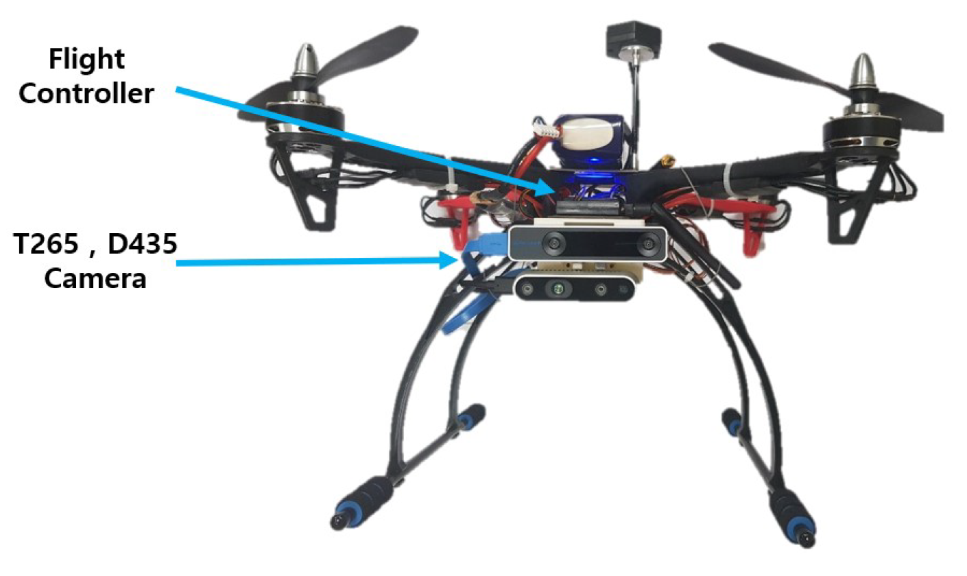
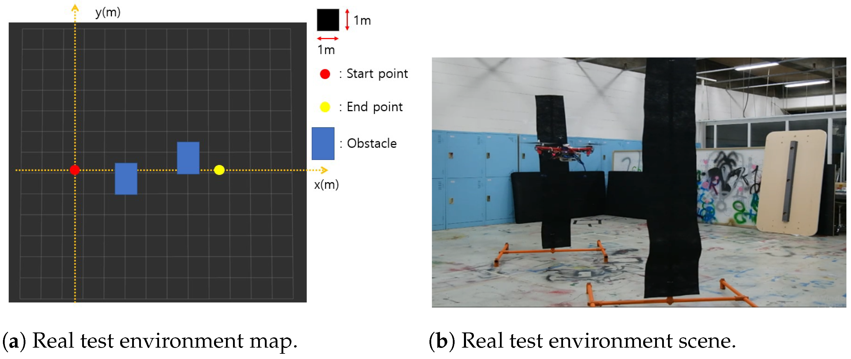
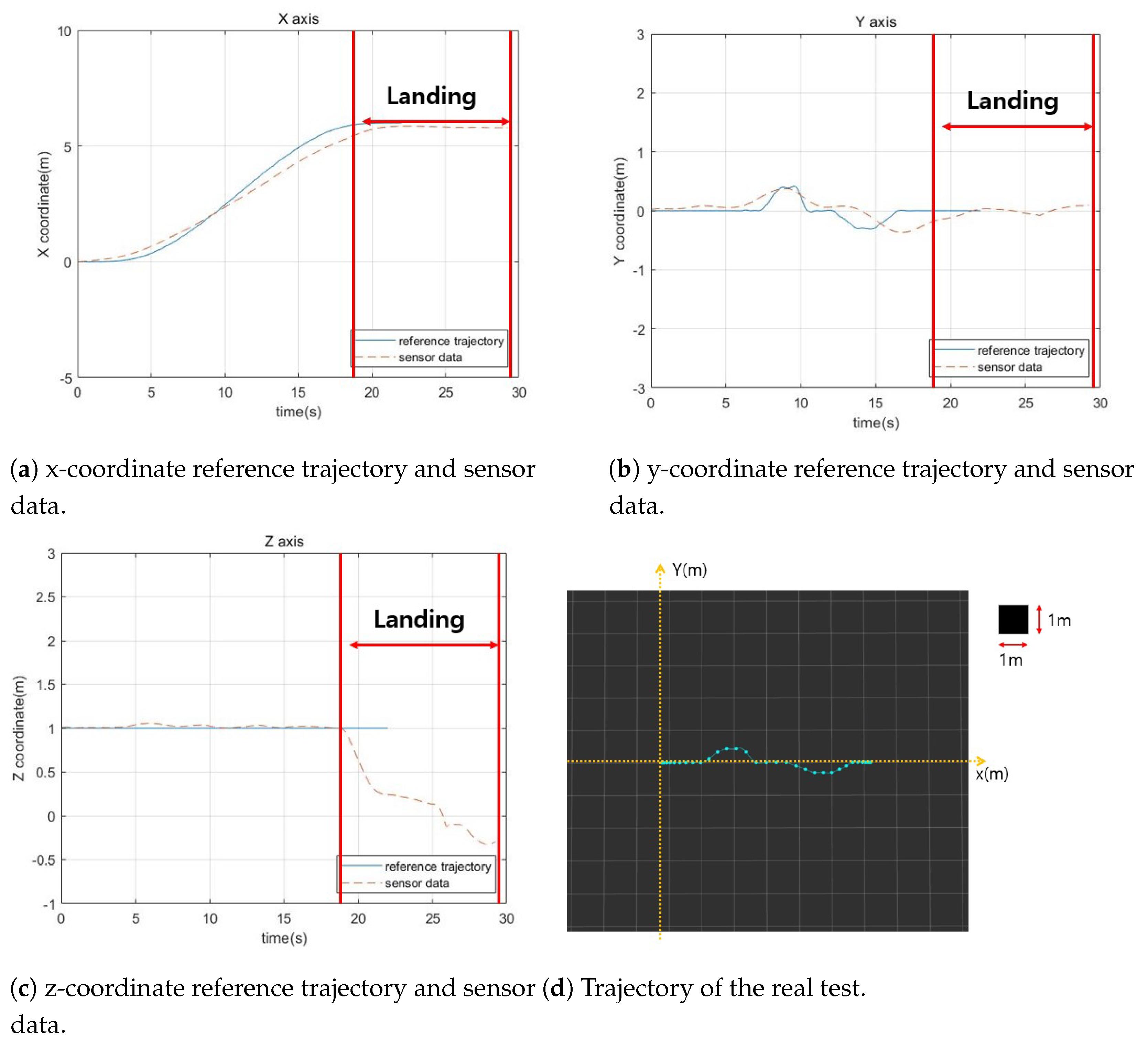
3.2. Experimental Results

After the simulation test, a real-life model of the quadrotor was assembled and set up with the hardware components. A DJI F450 frame and NVIDIA Jetson TX2 computer with J120 carrier board for high-level control and Pixhawk [17] for low-level control were used in this experiment. An Intel T265 camera was used to localize the quadrotor, and an Intel D435 camera for measuring depth to objects. The overall system is shown in Figure 10. The Jetson TX2 computer consists of a dual-core Denver2 CPU and quad-core ARM A57 CPU.

The on-board computer received data from the T265 and D435 cameras. After the on-board computer generated a trajectory, it transferred data to the Pixhawk flight controller with the MAVLink communication protocol. Then, PX4 conducted the tracking control, generating the desired rotor speeds, and sent the PWM (Pulse Width Modulation) signals to the motors. In this experiment, the quadrotor flew at a distance of about 6.5 m for 30 s The navigation environment and quadrotor flight are shown in Figure 11. The reference trajectory and sensor data are shown in Figure 12. The results of this experiment showed that the quadrotor successfully arrived at the end point without crashing.

4. Discussion and Conclusions

In this paper, the concept of trajectory generation where a quadrotor modifies its global trajectory and generates a local trajectory to avoid an obstacle in an unknown environment is covered and optimized. A new replanning method based on geometrical map information and closed-form formulation is proposed. This analytical solution can be computed much faster than other optimization methods because it does not conduct an iteration process. This closed-form method is free from local minima problems, and is thus safer and more robust than numerical methods. This method took 0.0000035 s for replanning, while other methods take about 0.03 s [11] or 0.00018 s [3] for replanning. This trajectory also considers dynamical and kinematic feasibility by using differential flatness and polynomial continuity. This trajectory generation method has strengths in computation speed, flying velocity, feasibility, non-collision, and resolution of local minima. It was tested both in simulation and in a real-world experiment, and it was proven that this algorithm is more robust and powerful than othersUsing a geometrical and analytical method, a safer and faster algorithm can be calculated allowing quadrotors to fly in messy and cluttered environments.

References

1. Yasin, J.N.; Mohamed, S.A.; Haghbayan, M.H.; Heikkonen, J.; Tenhunen, H.; Plosila, J. Unmanned aerial vehicles (uavs): Collision avoidance systems and approaches. IEEE Access 2020, 8, 105139–105155. [Google Scholar] [CrossRef]
2. Mellinger, D.; Kumar, V. Minimum snap trajectory generation and control for quadrotors. In Proceedings of the 2011 IEEE International Conference on Robotics and Automation, Shanghai, China, 9–13 May 2011; pp. 2520–2525. [Google Scholar]
3. Richter, C.; Bry, A.; Roy, N. Polynomial trajectory planning for aggressive quadrotor flight in dense indoor environments. In Robotics Research; Springer: Berlin/Heidelberg, Germany, 2016; pp. 649–666. [Google Scholar]
4. Copot, C.; Hernandez, A.; Mac, T.T.; De Keyse, R. Collision-free path planning in indoor environment using a quadrotor. In Proceedings of the 2016 21st International Conference on Methods and Models in Automation and Robotics (MMAR), Miedzyzdroje, Poland, 29 August–1 September 2016; pp. 351–356. [Google Scholar]
5. Penin, B.; Giordano, P.R.; Chaumette, F. Vision-based reactive planning for aggressive target tracking while avoiding collisions and occlusions. IEEE Robot. Autom. Lett. 2018, 3, 3725–3732. [Google Scholar] [CrossRef] [Green Version]
6. Oleynikova, H.; Taylor, Z.; Fehr, M.; Siegwart, R.; Nieto, J. Voxblox: Incremental 3d euclidean signed distance fields for on-board mav planning. In Proceedings of the 2017 IEEE/RSJ International Conference on Intelligent Robots and Systems (IROS), Vancouver, BC, Canada, 24–28 September 2017; pp. 1366–1373. [Google Scholar]
7. Taketomi, T.; Uchiyama, H.; Ikeda, S. Visual SLAM algorithms: A survey from 2010 to 2016. IPSJ Trans. Comput. Vis. Appl. 2017, 9, 1–11. [Google Scholar] [CrossRef]
8. Burri, M.; Oleynikova, H.; Achtelik, M.W.; Siegwart, R. Real-time visual-inertial mapping, re-localization and planning onboard mavs in unknown environments. In Proceedings of the 2015 IEEE/RSJ International Conference on Intelligent Robots and Systems (IROS), Hamburg, Germany, 28 September–3 October 2015; pp. 1872–1878. [Google Scholar]
9. Peng, X.Z.; Lin, H.Y.; Dai, J.M. Path planning and obstacle avoidance for vision guided quadrotor UAV navigation. In Proceedings of the 2016 12th IEEE International Conference on Control and Automation (ICCA), Kathmandu, Nepal, 1–3 June 2016; pp. 984–989. [Google Scholar]
10. Sanchez-Lopez, J.L.; Wang, M.; Olivares-Mendez, M.A.; Molina, M.; Voos, H. A real-time 3d path planning solution for collision-free navigation of multirotor aerial robots in dynamic environments. J. Intell. Robot. Syst. 2019, 93, 33–53. [Google Scholar] [CrossRef] [Green Version]
11. Oleynikova, H.; Burri, M.; Taylor, Z.; Nieto, J.; Siegwart, R.; Galceran, E. Continuous-time trajectory optimization for online UAV replanning. In Proceedings of the 2016 IEEE/RSJ international conference on intelligent robots and systems (IROS), Daejeon, Korea, 9–14 October 2016; pp. 5332–5339. [Google Scholar]
12. Betts, J.T. Survey of numerical methods for trajectory optimization. J. Guid. Control. Dyn. 1998, 21, 193–207. [Google Scholar] [CrossRef]
13. Gilmore, P.; Kelley, C.T. An implicit filtering algorithm for optimization of functions with many local minima. SIAM J. Optim. 1995, 5, 269–285. [Google Scholar] [CrossRef] [Green Version]
14. Yang, H.; Qi, J.; Miao, Y.; Sun, H.; Li, J. A new robot navigation algorithm based on a double-layer ant algorithm and trajectory optimization. IEEE Trans. Ind. Electron. 2018, 66, 8557–8566. [Google Scholar] [CrossRef] [Green Version]
15. Zhang, X.; Xian, B.; Zhao, B.; Zhang, Y. Autonomous flight control of a nano quadrotor helicopter in a GPS-denied environment using on-board vision. IEEE Trans. Ind. Electron. 2015, 62, 6392–6403. [Google Scholar] [CrossRef]
16. Furrer, F.; Burri, M.; Achtelik, M.; Siegwart, R. Robot Operating System (ROS): The Complete Reference (Volume 1); Springer International Publishing: Cham, Switzerland, 2016; pp. 595–625. [Google Scholar]
17. Meier, L.; Tanskanen, P.; Fraundorfer, F.; Pollefeys, M. Pixhawk: A system for autonomous flight using onboard computer vision. In Proceedings of the 2011 IEEE International Conference on Robotics and Automation, Shanghai, China, 9–13 May 2011; pp. 2992–2997. [Google Scholar]
18. Hornung, A.; Wurm, K.M.; Bennewitz, M.; Stachniss, C.; Burgard, W. OctoMap: An efficient probabilistic 3D mapping framework based on octrees. Auton. Robot. 2013, 34, 189–206. [Google Scholar] [CrossRef] [Green Version]
19. Lee, T.; Leok, M.; McClamroch, N.H. Geometric tracking control of a quadrotor UAV on SE (3). In Proceedings of the 49th IEEE conference on decision and control (CDC), Atlanta, GA, USA, 15–17 December 2010; pp. 5420–5425. [Google Scholar]
20. Usenko, V.; Von Stumberg, L.; Pangercic, A.; Cremers, D. Real-time trajectory replanning for MAVs using uniform B-splines and a 3D circular buffer. In Proceedings of the 2017 IEEE/RSJ International Conference on Intelligent Robots and Systems (IROS), Vancouver, BC, Canada, 24–28 September 2017; pp. 215–222. [Google Scholar]
Figure 1. Local trajectory generation.
Applsci 11 03238 g001
Figure 2. Time-scaling.
Applsci 11 03238 g002
Figure 3. Trajectory replanning.
Applsci 11 03238 g003
Figure 4. Smoothing trajectory.
Applsci 11 03238 g004
Figure 5. Required acceleration of trajectory.
Applsci 11 03238 g005
Figure 6. Cluttered environment in the simulation.
Applsci 11 03238 g006
Figure 7. Occupancy grid (red), local trajectory (green), and global trajectory (purple).
Applsci 11 03238 g007
Figure 8. Reference trajectory and sensor data graph of the trajectory.
Applsci 11 03238 g008
Figure 9. Replanning of global trajectory.
Applsci 11 03238 g009
Figure 10. Quadrotor front view.
Applsci 11 03238 g010
Figure 11. Real test.
Applsci 11 03238 g011
Figure 12. Reference trajectory and sensor data graph of the real test.
Applsci 11 03238 g012