Geometric Reduced-Attitude Control of Fixed-Wing UAVs

Featured Application

Although the focus in this article is on unmanned aerial vehicles, the geometric reduced-attitude controllers presented apply to all fixed-wing aircraft with fully actuated rotational dynamics. The proposed approach could also be applied to other bank-to-turn vehicles such as missiles. The method can be particularly useful for situations where the vehicle experiences large deviations from the attitude reference.

Abstract

This paper presents nonlinear, singularity-free autopilot designs for multivariable reduced-attitude control of fixed-wing aircraft. To control roll and pitch angles, we employ vector coordinates constrained to the unit two-sphere and that are independent of the yaw/heading angle. The angular velocity projected onto this vector is enforced to satisfy the coordinated-turn equation. We exploit model structure in the design and prove almost global asymptotic stability using Lyapunov-based tools. Slowly-varying aerodynamic disturbances are compensated for using adaptive backstepping. To emphasize the practical application of our result, we also establish the ultimate boundedness of the solutions under a simplified controller that only depends on rough estimates of the control-effectiveness matrix. The controller design can be used with state-of-the-art guidance systems for fixed-wing unmanned aerial vehicles (UAVs) and is implemented in the open-source autopilot ArduPilot for validation through realistic software-in-the-loop (SITL) simulations.

1. Introduction

1.1. Background and Motivation

In recent years, technology advancements have led to increased use of small unmanned aerial vehicles (UAVs) in civil, commercial, and scientific applications. Fixed-wing UAVs [1], as illustrated in Figure 1, have superior range and endurance when compared to rotary-wing UAVs, which enable applications such as environmental monitoring, search and rescue, aerial surveillance and mapping, and medical transportation [2]. To further develop the field, and enable safe and efficient autonomous operation of UAVs, requires robust autopilots that can handle a range of environmental conditions, including turbulent wind conditions, and operate in the presence of highly uncertain aerodynamics [3].

Figure 1. Skywalker X8 fixed-wing UAV (Image courtesy of NTNU UAV-Lab).

As underactuated vehicles, conventional fixed-wing aircraft have fewer control inputs than the dimension of their configuration space. One or more propellers provide a thrust-force in the longitudinal direction, but the forces orthogonal to the thrust axis (lift, side-force) are not directly controllable. Therefore, fixed-wing UAVs have to resort to using guidance schemes [4], where the UAV’s geometric path in 3-D space is controlled by specifying course and flight path angle commands to lower-level autopilots [5]. Due to the fact that small fixed-wing UAVs experience winds that are large relative to their operating airspeeds [1], path-following methods [6] are usually preferred over trajectory tracking control [7]. In path following, the goal is to reach and follow a geometric path, but without any temporal constraints. This also deals with performance limitations of trajectory tracking for systems with nonminimum phase characteristics, such as aircraft [8]. See [9,10] for a comparison of different path-following algorithms for fixed-wing UAVs, in two and three dimensions, respectively. For a recent survey with a focus on quadrotor UAVs, see [11].

Guidance and control systems for unmanned vehicles can be integrated, or separated [12]. For integrated guidance and control (IGC) systems, the guidance system and inner-loop autopilot are designed simultaneously, taking cross-coupling effects into account. On the other hand, in separated guidance and control (SGC), inner and outer loops are designed separately, with modularity and cross-platform use in mind [13]. Examples of separate guidance algorithms for fixed-wing UAVs include nonlinear guidance laws [14,15], vector-field path following [16,17] and a guidance law based on nested saturations [18]. In [19], path following is achieved by using an existing commercial inner-loop autopilot but augmented with an ${\mathcal{L}}_1$ adaptive controller to deal with modeling uncertainty and environmental disturbances. While most guidance algorithms use only kinematic models, an integrated approach is presented in [20] that uses a simple model of the aerodynamic forces acting on the aircraft. Common to all the mentioned approaches, both IGC and SGC, is the reliance on attitude control in the inner-most loop. The rotational dynamics is not considered but rather assumed to be stabilized by some low-level controller. This motivates further research on attitude controllers, specifically tailored towards fixed-wing UAVs.

Several different attitude representations have been employed for fixed-wing UAV path following, including Euler angles [21], rotation matrices [22] and unit quaternions [23]. Minimal representations such as Euler angles are often used because of their intuitive interpretation but suffer from “gimbal-lock” singularities [24]. Unit quaternions [25] are singularity-free, but provide a double cover of $\mathrm{SO}\left(3\right)$, the space of 3-D rotations. This might lead to unwinding, where the UAV unnecessarily makes a full rotation, even when arbitrarily close to the target attitude [26,27]. Rotation matrices, on the other hand, provide a global and unique representation. This has led to a significant research effort into so-called geometric attitude control, where singularity-free controllers are designed directly on $\mathrm{SO}\left(3\right)$, using rotation matrices, that avoid the unwinding phenomenon and often controls the system along geodesics, i.e., paths of minimum length in rotation space [28,29,30,31,32,33]. These advantages are desirable when the controlled vehicle is subject to large angle rotations, e.g., a fixed-wing UAV recovering from large attitude errors resulting from severe wind gusts [34].

Fixed-wing UAVs use one of two main mechanisms for turning: bank-to-turn, where a lateral acceleration is generated by reorienting the lift-force by rolling/banking the UAV, or skid-to-turn, where turning is achieved by generating a sideslip angle, which in turn generates a lateral force that turns the vehicle [35]. In [36], these methods are combined to reduce lateral distortion of camera images gathered by a fixed-wing UAV. In general, bank-to-turn is often preferred over skid-to-turn because for most aircraft the lift force is of orders of magnitude greater than thrust forces [37]. Thus, the course angle, yaw angle, and turn rate of aircraft are not controlled directly, but rather through banked-turn maneuvers. For aircraft in coordinated turns, i.e., with zero sideslip angle, the coordinated-turn equation provides a simple relationship between roll angle and resulting turn rate, and is for this reason often used in autopilot design [1,38,39,40,41,42], including those used in state-of-the-art open-source autopilots [43,44].

Controllers designed using rotation matrices or quaternions control the full attitude, and therefore cannot be directly applied to fixed-wing aircraft using banked turn maneuvers. One approach could be to feedback the true yaw angle into the desired rotation matrix and as such use a rotation error representation for roll and pitch only. However, this representation is highly redundant, as 9 parameters are used to parametrize a two-dimensional subspace. A simpler approach, that does not require the full machinery of working in $\mathrm{SO}\left(3\right)$, is to consider a reduced-attitude representation, evolving on the two-sphere, ${\mathbb{S}}^2\subset {\mathbb{R}}^3$ [45]. In this space of reduced attitude, all rotations that are related by a rotation about some fixed axis, are considered the same [27]. Control systems with reduced attitude evolving on ${\mathbb{S}}^2$ have previously been studied in the context of spin-axis [45] and boresight-axis [46] control for satellites, pendulum stabilization [31], path-following control of underwater vehicles [47], thrust-vector control for multirotor UAVs [48,49] and for general rigid bodies [50,51,52]. Controllers developed on ${\mathbb{S}}^2$ are relatively simple compared to those developed using rotation matrices and require fewer matrix operations.

It is well known that a desired attitude (full or reduced) cannot be globally stabilized using continuous state-feedback control laws [26]. This stems from the topological properties of $\mathrm{SO}\left(3\right)$ and ${\mathbb{S}}^2$, which are compact, boundaryless manifolds that are not diffeomorphic to any Euclidean space. The largest possible attraction basins under continuous feedback are almost global, i.e., excluding a zero-measure set, which corresponds to the stable manifolds of additional unstable equilibrium points [53]. However, global asymptotic stability can be achieved by using tools from hybrid dynamical systems, where hysteresis-based switching ensures that all trajectories converge to the desired equilibrium [49,50,52,54,55,56,57].

1.2. Scope and Contributions

In this paper, we present smooth, nonlinear reduced-attitude controllers for fixed-wing UAVs, in a coordinate-free manner, using a global, singularity-free attitude representation on ${\mathbb{S}}^2$. The method applies to UAVs with fully actuated rotational dynamics, e.g., those that are equipped with a full set of control surfaces, such as ailerons, elevator, and rudder. The chosen reduced-attitude representation is independent of the yaw angle and thus enables traditional banked-turn maneuvers. A consequence of this is that the presented approach can be deployed in conjunction with state-of-the-art hierarchical flight control architectures that rely on roll and pitch control in the inner loop, such as [1], and those implemented in open-source autopilots such as ArduPilot [43] and PX4 [44]. Furthermore, no lateral/longitudinal decoupling assumptions are used in the design, allowing the attitude controller to compensate for coupling effects that arise when such assumptions are violated.

The reduced-attitude representation allows for a convenient decomposition of the dynamics and a natural corresponding decoupling of the control objective into two parts: (1) reduced-attitude (roll/pitch) control, and (2) control of the angular velocity about the inertial z-axis (turn rate control). Using Lyapunov theory, almost global asymptotic stability is established for three controllers: one constructed based on an energy-like Lyapunov function, a variation of this based on a backstepping procedure, and lastly an adaptive version of the latter that estimates the net aerodynamic moment caused by the translational dynamics (flow angles). This alleviates the need for expensive flow angle measurement equipment, as well as the knowledge of an accurate aerodynamic model. Furthermore, we show that only a rough estimate of the input matrix is needed to achieve ultimate boundedness. The suitability of the proposed attitude control algorithm is demonstrated in realistic software-in-the-loop simulations.

1.3. Related Work

The existing work in the literature that shares the most similarities with this paper can be found in [58,59,60,61], where nonlinear attitude controllers for fixed-wing UAVs are developed using quaternions, and that also use a model of the rotational dynamics. In [58,59], the translational and rotational subsystems are decoupled by estimating the higher-order derivatives of the angle of attack and sideslip angle. This enables controllers for the two subsystems to be designed separately. In [60], a nonlinear PID controller for fixed-wing UAV (full) attitude control is presented. The control law is based on unit quaternions and compensates for aerodynamic coupling effects using integral action. This approach is extended in [61] to apply also to rudderless (i.e., underactuated in attitude) fixed-wing UAVs by using a projection of the quaternion error to a yaw-free subspace. In [62], a gain-scheduled attitude controller based on Euler angles is given. An algorithm for automatic tuning is provided, and the control system is verified experimentally in a wind tunnel.

Reduced-attitude control has been extensively applied for thrust-vector control of multirotor UAVs, e.g., [48]. Fixed-wing UAVs on the other hand, are subject to additional aerodynamic forces and moments that make control of such vehicles fundamentally different. Besides, the reduced-attitude representation used in this paper (gravity direction represented in body-fixed frame) is different than the thrust-direction of multirotors (body-fixed axis represented in the inertial frame). The representation used here is similar to that used to stabilize the inverted equilibrium manifold of the 3-D pendulum in [31,63].

The idea of separately controlling reduced attitude and another variable that is decoupled from the reduced-attitude vector is not new. In [64], the reduced attitude is steered along a geodesic path, while the full attitude is stabilized. In [65,66], the attitude control of a quadrotor is decoupled into thrust-vector control on ${\mathbb{S}}^2$, and control of the angle of rotation about the thrust vector. A similar approach is taken in [67] with a control allocation strategy that allows to prioritize reduced-attitude correction over yaw errors. Different rotational error metrics for quadrotor control, defined in terms of both full and reduced attitude are compared in [68]. In [69], a vector-projection algorithm is used for trajectory tracking for an agile fixed-wing UAV (where aerodynamics are dominated by the propeller). The roll angle is decoupled from the reference attitude such that thrust and lift forces can be pointed such that position tracking is achieved. Compared to these works, we simultaneously control reduced attitude and an angular velocity around the reduced-attitude vector.

While the present work employs Lyapunov-based methods to develop lightweight control laws with stability guarantees, other approaches using optimal control algorithms have also been proposed, using deep reinforcement learning [70] and nonlinear model predictive control [71].

Preliminary results of the work presented in this paper have previously been reported in [72], and some initial work towards extending this by applying tools from hybrid control can be found in [73].

1.4. Organization of the Paper

The rest of the paper is organized as follows: Section 2 presents some notation and preliminaries on the reduced-attitude representation. The UAV equations of motion are given in Section 3, and the control objective is stated in Section 4 along with the definitions of the error functions used. In Section 5, the controllers for the nominal model are presented. Some robustness considerations are stated in Section 6, where we also give an adaptive version of the backstepping-based control law. The simulation results are presented in Section 7, and some concluding remarks are given in Section 8. All lengthy proofs have been relegated to the appendices.

2. Preliminaries

In this section, we establish some notation and useful mathematical relations that are used throughout the text, before presenting the reduced-attitude representation.

2.1. Notation and Definitions

For $a\in \mathbb{R}$ and $x\in {\mathbb{R}}^n$, let $\left|a\right|$ and $\parallel x\parallel =\sqrt{x^{\top }x}$ denote the absolute value and the Euclidean norm, respectively. Positive (resp. non-negative) real numbers are denoted ${\mathbb{R}}_{+}$ (${\mathbb{R}}_{\ge 0}$), and the maximum and minimum eigenvalues of a square matrix A is denoted ${\lambda }_{max}\left(A\right)$, ${\lambda }_{min}\left(A\right)$, respectively. The induced 2-norm of a matrix A is $\parallel A\parallel ={\sigma }_{max}\left(A\right)$, where ${\sigma }_{max}\left(A\right)$ is the largest singular value of A. For square, real symmetric positive semidefinite matrices A, ${\lambda }_{max}\left(A\right)={\sigma }_{max}\left(A\right)$. Any square matrix A can be written as the sum of a symmetric and skew symmetric part, $A=sym\left(A\right)+skew\left(A\right)$, where $sym\left(A\right)=(A+A^{\top })/2$ and $skew\left(A\right)=(A-A^{\top })/2$. For a symmetric matrix $A=A^{\top }$, we have the following inequality for quadratic forms: ${\lambda }_{min}{\parallel x\parallel }^2\le x^{\top }Ax\le {\lambda }_{max}{\parallel x\parallel }^2$.

For any $u,v\in {\mathbb{R}}^3$, the matrix $S\left(u\right)=-S^{\top }\left(u\right)\in \mathrm{so}\left(3\right)$ is the skew-symmetric matrix such that $S\left(u\right)v=u\times v$. From properties of the cross product we have $S\left(u\right)v=-S\left(v\right)u$, $S\left(u\right)u=0$ and $u^{\top }S\left(v\right)u=0$, which implies that $u^{\top }Au=u^{\top }sym\left(A\right)u$ for any square matrix A.

We make use of standard right-handed coordinate frames: $\left\{n\right\}$, a local north-east-down tangent frame (assumed inertial), and $\left\{b\right\}$, a body-fixed frame centered at the center of gravity of the UAV, with the x-axis in the longitudinal direction and the y-axis pointing towards the right wing.

The three-dimensional special orthogonal group is the set of three-dimensional rotation matrices, given by

$$\mathrm{SO}\left(3\right)=\{R\in {\mathbb{R}}^{3\times 3}:R^{\top }R=I_3,detR=1\},$$

where $I_3\in {\mathbb{R}}^{3\times 3}$ is the identity matrix. The two-sphere ${\mathbb{S}}^2\subset {\mathbb{R}}^3$ is defined by

$${\mathbb{S}}^2=\{x\in {\mathbb{R}}^3:\parallel x\parallel =1\}.$$

The tangent space at a point $x\in {\mathbb{S}}^2$ can be identified with the vectors that are orthogonal to x:

$${\mathrm{T}}_x{\mathbb{S}}^2=\{v\in {\mathbb{R}}^3:x^{\top }v=0\},$$

and the normal space ${\mathrm{N}}_x{\mathbb{S}}^2$ is the set of vectors parallel to x:

$${\mathrm{N}}_x{\mathbb{S}}^2=\{w\in {\mathbb{R}}^3:w^{\top }v=0\mathrm{for}\mathrm{all}v\in {\mathrm{T}}_x{\mathbb{S}}^2\}.$$

Define the orthogonal and parallel projections ${\Pi }_x^{\perp }:{\mathbb{R}}^3\to {\mathrm{T}}_x{\mathbb{S}}^2$ and ${\Pi }_x^{\Vert }:{\mathbb{R}}^3\to {\mathrm{N}}_x{\mathbb{S}}^2$ by

$${\Pi }_x^{\perp }=I_3-x{x}^{\top }=-S^2\left(x\right),{\Pi }_x^{\Vert }=x{x}^{\top }.$$

(1)

Then, any vector $v\in {\mathbb{R}}^3$ can be written as the sum $v={\Pi }_x^{\perp }v+{\Pi }_x^{\Vert }v$.

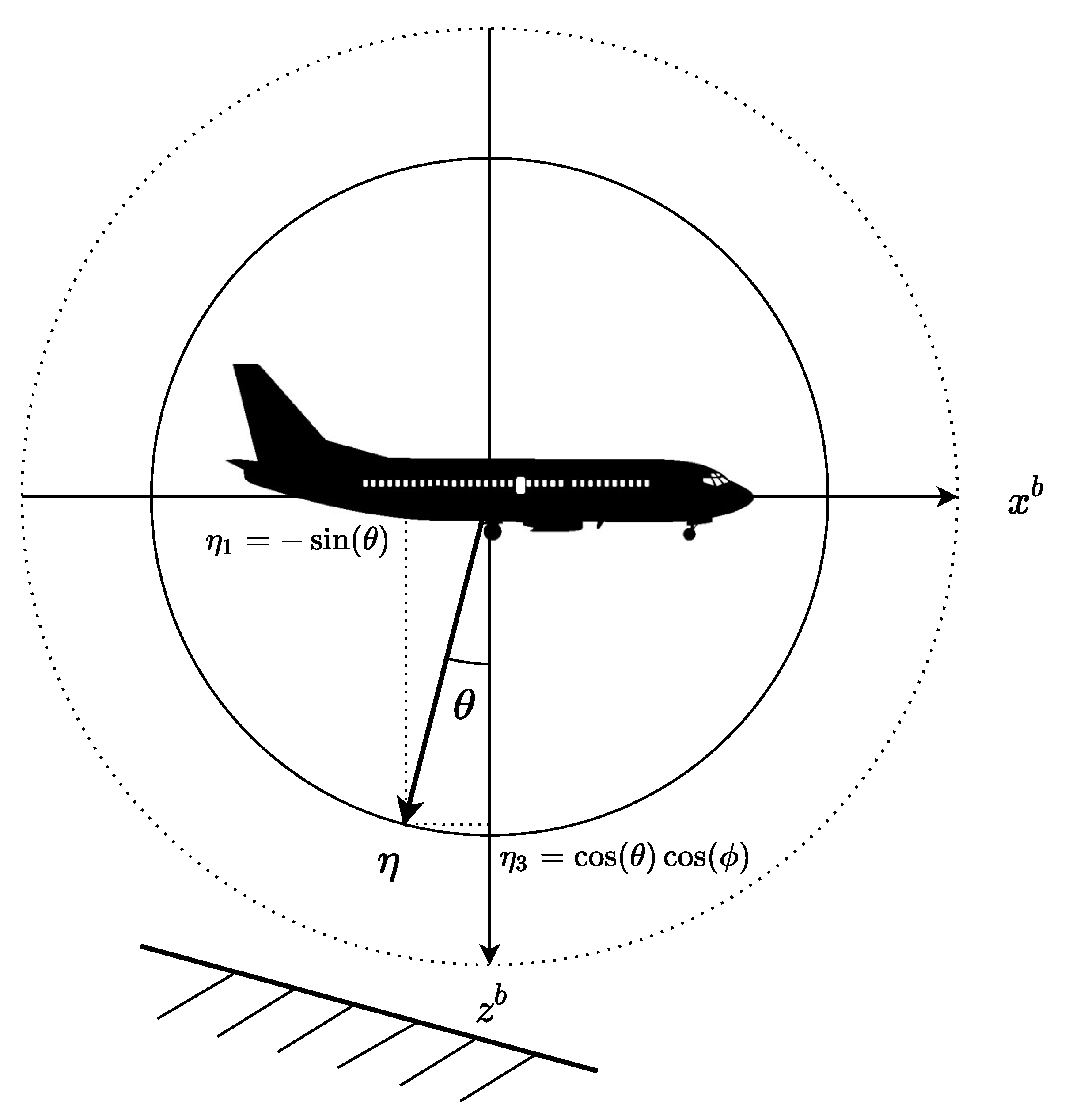
2.2. Reduced-Attitude Representation

Let $R\in \mathrm{SO}\left(3\right)$ be the rotation matrix transforming vectors from $\left\{b\right\}$ to $\left\{n\right\}$, and let $e_3={\left[001\right]}^{\top }$ represent the inertial z-direction (direction of gravitational acceleration). We employ the following reduced-attitude representation:

$$\eta =R^{\top }{e}_3\in {\mathbb{S}}^2,$$

(2)

which is interpreted as the inertial z-axis, expressed in $\left\{b\right\}$. By expanding (2) using the roll-pitch-yaw Euler-angle parametrization of R [1], the reduced-attitude vector $\eta$ can be expressed in terms of the roll angle $\varphi \in [-\pi ,\pi ]$ and pitch angle $\theta \in (-\pi /2,\pi /2)$ as follows:

$$\eta =\left[\begin{array}{c}-sin\left(\theta \right)\\ cos\left(\theta \right)sin\left(\varphi \right)\\ cos\left(\theta \right)cos\left(\varphi \right)\end{array}\right].$$

(3)

Observe that this particular choice of attitude representation is invariant to changes in the heading/yaw angle $\psi$. The reduced attitude representation is illustrated in Figure 2, where a section of the sphere corresponding to $\theta =0$ is shown. Figure 3 shows another section where the aircraft is shown from the side with a possible nonzero roll angle. As shown, the vector $\eta$ is expressed in the body-fixed frame and points towards the ground.

Figure 2. Reduced-attitude representation illustrated with a section of the two-sphere corresponding to $\theta =0$.

Figure 3. Reduced-attitude representation. The aircraft is shown from the side, illustrated with a section of the two-sphere possibly with a non-zero roll angle.

The reduced-attitude representation (2) is the same as the one considered for the 3-D pendulum in [31], but different compared to the one used for thrust-vector control for multirotor UAVs, which is the thrust direction in the inertial-frame [48].

Let $\omega \in {\mathbb{R}}^3$ be the angular velocity of the body-fixed frame relative to the inertial frame, expressed in the body-fixed frame. The reduced-attitude vector $\eta$ satisfies

$$\dot{\eta }=\eta \times \omega ,$$

(4)

which can be derived from (2) and the relation $\dot{R}=RS\left(\omega \right)$ [74].

Using (1), we can perform an orthogonal decomposition of the angular velocity $\omega$ with respect to $\eta$ such that $\omega ={\omega }^{\perp }+{\omega }^{\Vert }$, where

$${\omega }^{\perp }\triangleq {\Pi }_{\eta }^{\perp }\omega \in {\mathrm{T}}_{\eta }{\mathbb{S}}^2{\omega }^{\Vert }\triangleq {\Pi }_{\eta }^{\Vert }\omega \in {\mathrm{N}}_{\eta }{\mathbb{S}}^2.$$

(5)

Applying this decomposition of $\omega$ in combination with (4) gives

$$\dot{\eta }=\eta \times ({\omega }^{\perp }+{\omega }^{\Vert })=\eta \times {\omega }^{\perp }.$$

(6)

The parallel component ${\omega }^{\Vert }$ is the angular velocity about the inertial z-axis (expressed in the body-fixed frame) and does not influence $\dot{\eta }$.

Remark 1.

Note that since the two-sphere ${\mathbb{S}}^2$ is a two-dimensional manifold, in principle two degrees of freedom (DOFs) are sufficient to control reduced attitude. However, since η is fixed in the inertial frame, the two required DOFs (control directions) vary with the orientation of the vehicle and are thus not fixed in $\left\{b\right\}$. Therefore, we need three actuators to make the reduced attitude fully controllable throughout the configuration space. In this paper, we consider only UAVs with fully actuated rotational dynamics, and at each time instant, we use the remaining DOF to control ${\omega }^{\Vert }$.

3. UAV Rotational Dynamics

A standard dynamic model of the rigid-body rotational dynamics is given by the Euler equations [1]

$$J\dot{\omega }+\omega \times J\omega =M,$$

where $J=J^{\top }>0$ is the inertia matrix and $M\in {\mathbb{R}}^3$ is a vector of applied torques, typically a sum of aerodynamic and propulsion effects. In this respect, we write $M=M_a+M_p$, where $M_a$ denotes the aerodynamic torque, while $M_p$ is caused by a rotating propeller.

3.1. Aerodynamics

Aerodynamic forces and moments are in general nonlinear functions that are difficult to model accurately. Identification of parameters for even simple linear models from flight data remains a challenging problem [75,76]. Following [1,77] we define the aerodynamic torque as a function of the angular velocity $\omega$, the body-fixed relative velocity $v_r\in {\mathbb{R}}^3$ of the UAV (with respect to the surrounding air mass), and a vector $u\in {\mathbb{R}}^3$ of control surface deflections used to control the attitude of the UAV:

$$M_a=M_a(\omega ,v_r,u).$$

Reynolds and Mach number effects are usually ignored for small UAVs moving at airspeeds well below the speed of sound [1].

The airspeed $V_a\in {\mathbb{R}}_{\ge 0}$, angle of attack $\alpha \in [-\pi ,\pi ]$ and sideslip angle $\beta \in [-\pi ,\pi ]$ are defined by

$$V_a=\parallel v_r\parallel =\sqrt{v_{r_1}^2+v_{r_2}^2+v_{r_3}^2}$$

$$\alpha =atan2\left(v_{r_3},v_{r_1}\right),\beta =atan2\left(v_{r_2},v_{r_1}\right),$$

where $atan2(y,x)$ is the four-quadrant inverse tangent.

Let $\rho ,b,c,S\in {\mathbb{R}}_{+}$ be the air density, wingspan, mean wing chord, and wing planform area of the UAV, respectively. A first approximation of the aerodynamic moments that is commonly used in the literature [1,77], and can be useful for control design is given by the control-affine model

$$M_a(\omega ,v_r,u)=h\left(v_r\right)+V_{a}D\omega +V_a^{2}Bu,$$

with

$$\begin{array}{cc}\hfill h\left(v_r\right)& =\frac{\rho V_a^{2}S}{2}\left[\begin{array}{c}b{C}_{l_{\beta }}\beta \\ c(C_{m_0}+C_{m_{\alpha }}\alpha )\\ b{C}_{n_{\beta }}\beta \end{array}\right]\hfill \\ \hfill D& =\frac{\rho S}{4}\left[\begin{array}{ccc}{b}^2{C}_{l_p}& 0& b^2{C}_{l_r}\\ 0& c^2{C}_{m_q}& 0\\ b^2{C}_{n_p}& 0& b^2{C}_{n_r}\end{array}\right]\hfill \\ \hfill B& =\frac{\rho S}{2}\left[\begin{array}{ccc}b{C}_{l_{{\delta }_a}}& 0& b{C}_{l_{{\delta }_r}}\\ 0& c{C}_{m_{{\delta }_e}}& 0\\ b{C}_{n_{{\delta }_a}}& 0& b{C}_{n_{{\delta }_r}}\end{array}\right],\hfill \end{array}$$

where the parameters $C_{\left(·\right)}$ are dimensionless aerodynamic coefficients.

3.2. Propulsion Effects

Let ${\Omega }_p\in \mathbb{R}$ be the rotational speed of the propeller, given in radians per second, and without loss of generality, assume that the propeller thrust axis is aligned with the body-frame x axis. Following [1], for some constant $k_{\Omega }\in \mathbb{R}$, we write

$$\begin{array}{c}\hfill M_p=\left[\begin{array}{c}{k}_{\Omega }{\Omega }_p^2\\ 0\\ 0\end{array}\right].\end{array}$$

This is a reaction torque caused by the motor of the UAV. Since the motor torque is bounded, we can write $\parallel M_p\parallel \le c_{\Omega }$. If the propeller axis is not properly aligned with the x-axis of the body frame, we will get additional small non-zero elements in $M_p$, but the bound still holds for some $c_{\Omega }$. If we also consider a gyroscopic torque (typically small, but sometimes actually used to control aircraft attitude, see Lomcevak maneuver [78]), the subsequent analysis must be adjusted slightly, since the gyroscopic moment also depends on the angular velocity of the UAV. Instead of considering $M_p$ as a bounded time-varying exogenous signal, we could then write $\parallel M_p\parallel \le a+b\parallel \omega \parallel$ for suitable constants a and b. Additional modeling of complex phenomena generated by the interplay between the main body of the UAV and its propeller (slipstream effects) can be found in [79].

3.3. Control-Oriented Model

To summarize, the UAV rotational dynamics can be written

$$J\dot{\omega }=S\left(J\omega \right)\omega +h\left(v_r\right)+V_{a}D\omega +V_a^{2}Bu+M_p.$$

(7)

In horizontal, level flight, the angular velocity $\omega$ is zero. To ensure equilibrium flight (“trim conditions”), define

$$u_{\mathrm{trim}}=\frac{1}{{\left(V_a^{*}\right)}^2}{B}^{-1}\left[-h\left(v_r^{*}\right)-M_p^{*}\right],$$

where $V_a^{*}$, $v_r^{*}$, $M_p^{*}$ is the trim airspeed, trim relative velocity and trim propeller moment (corresponding to the trim throttle setting), respectively. If $u=u_{\mathrm{trim}}$ and $\omega =0$, then $\dot{\omega }=0$ during trimmed flight. Now define

$$\Delta (v_r,t)=V_a^{2}B{u}_{\mathrm{trim}}+h\left(v_r\right)+M_p$$

(8)

which represents the deviation from trimmed flight. We can now combine (8), the rotational dynamics (7) and the reduced-attitude kinematics (4) to obtain the following model that is the basis for control design:

$$\begin{array}{cc}\hfill \dot{\eta }& =\eta \times \omega \hfill \end{array}$$

(9)

$$\begin{array}{cc}\hfill J\dot{\omega }& =S\left(J\omega \right)\omega +V_{a}D\omega +V_a^{2}B\left[u-u_{\mathrm{trim}}\right]+\Delta (v_r,t).\hfill \end{array}$$

(10)

The state is represented by $(\eta ,\omega )\in {\mathbb{S}}^2\times {\mathbb{R}}^3$, the control input is $u\in {\mathbb{R}}^3$, and we consider $v_r$ (and thus $V_a$) as an exogenous bounded input.

To fascilitate control design, we will assume the following:

Assumption A1.

The airspeed $V_a$ is strictly positive and bounded with bounded derivative $0<V_{min}\le V_a\le V_{max}$.

Assumption A2.

The moment vector $\Delta (v_r,t)$ and its derivative $\dot{\Delta }(v_r,t)$ are bounded.

Assumption A3.

The control effectiveness matrix B is invertible.

Assumption A4.

The damping matrix D satisfies $x^{\top }Dx\le 0,\forall x\in {\mathbb{R}}^3$.

Remark 2.

Assumption 2 is an assumption on the translational dynamics, which is assumed to affect the rotational dynamics through the exogenous signal $v_r$ (may also be considered as “internal dynamics”). In practice, since we are dealing with a physical system, $\Delta (v_r,t)$ and $\dot{\Delta }(v_r,t)$ will always be of bounded magnitude. However, since the control input is bounded, we would want these bounds to be relatively small. In particular, during nominal flight, the angle of attack α is usually small, and the lift coefficient is such that a perturbation in α tends to be restored [1]. However, if the stall angle of attack is reached, the slope of the lift coefficient changes such that the α-dynamics might go unstable, which in turn results in a high aerodynamic moment $\Delta (v_r,t)$.

Remark 3.

A square matrix B corresponds to a fixed-wing UAV that has fully actuated rotational dynamics, i.e., three independent actuators. Now B is invertible if it has full rank. It can be shown that the full rank condition corresponds to primary control coefficients being larger than the coefficients associated with secondary roll-yaw coupling effects. The full rank assumption is therefore reasonable for most common fully actuated control surface configurations.

Remark 4.

Assumption 4 is a dissipation assumption and is equivalent to requiring that $sym\left(D\right)$ has nonpositive eigenvalues. In nominal flight conditions, this will be true for most airframes [77] but can be relaxed by using a higher derivative gain (adding damping to the system). See Remark 8.

4. Almost Global Reduced-Attitude Tracking Control for Fixed-Wing UAVs

4.1. Error Functions

The goal is to design a state-feedback control law $u\in {\mathbb{R}}^3$ to make the reduced attitude $\eta \in {\mathbb{S}}^2$ asymptotically track a smooth, time-varying reference ${\eta }_d\in {\mathbb{S}}^2$ and at the same time drive ${\omega }^{\Vert }$ to ${\omega }_d^{\Vert }$, where ${\omega }_d^{\Vert }\in {\mathrm{N}}_{\eta }{\mathbb{S}}^2$ denotes the desired value of ${\omega }^{\Vert }$, yet to be specified. Furthermore, let the desired reduced-attitude vector ${\eta }_d$ satisfy the reference model

$$\begin{array}{cc}\hfill {\dot{\eta }}_d& ={\eta }_d\times {\omega }_d^{\perp },\hfill \end{array}$$

(11)

where ${\omega }_d^{\perp }\in {\mathrm{T}}_{{\eta }_d}{\mathbb{S}}^2$.

Assumption A5.

The angular velocity references ${\omega }_d^{\perp }$, ${\omega }_d^{\Vert }$ and their derivatives ${\dot{\omega }}_d^{\perp }\triangleq \frac{d}{dt}{\omega }_d^{\perp }$, ${\dot{\omega }}_d^{\Vert }\triangleq \frac{d}{dt}{\omega }_d^{\Vert }$ can be bounded a priori by

$$\begin{array}{cccc}\hfill \parallel {\omega }_d^{\Vert }\parallel & \le c_{{\omega }_d^{\Vert }}\hfill & \hfill \parallel {\dot{\omega }}_d^{\Vert }\parallel & \le b_{{\dot{\omega }}_d^{\Vert }}\parallel \omega \parallel +c_{{\dot{\omega }}_d^{\Vert }}\hfill \\ \hfill \parallel {\omega }_d^{\perp }\parallel & \le c_{{\omega }_d^{\perp }}\hfill & \hfill \parallel {\dot{\omega }}_d^{\perp }\parallel & \le c_{{\dot{\omega }}_d^{\perp }},\hfill \end{array}$$

(12)

where $c_{{\omega }_d^{\Vert }},c_{{\dot{\omega }}_d^{\Vert }},c_{{\omega }_d^{\perp }},c_{{\dot{\omega }}_d^{\perp }},b_{{\dot{\omega }}_d^{\Vert }}\in {\mathbb{R}}_{+}$ are appropriate constant parameters.

Let a smooth configuration error function $\Psi :{\mathbb{S}}^2\times {\mathbb{S}}^2\to \mathbb{R}$ be defined by

$$\Psi (\eta ,{\eta }_d)=1-{\eta }_d^{\top }\eta =1-cos\nu ,$$

(13)

where $\nu$ is the angle between $\eta$ and ${\eta }_d$. The function $\Psi$ measures the “distance” between two points $\eta$ and ${\eta }_d$ on ${\mathbb{S}}^2$, and is clearly positive definite with respect to $\eta ={\eta }_d$. There are two critical points: A minimum when $\eta ={\eta }_d$, and a maximum when $\eta =-{\eta }_d$. In subsequent Lyapunov analysis, $\Psi$ is used as a pseudo-potential energy term in Lyapunov functions.

We proceed by defining the following error vectors:

$$\begin{array}{cc}\hfill e_{\eta }& \triangleq \eta \times {\eta }_d\in {\mathrm{T}}_{\eta }{\mathbb{S}}^2\hfill \end{array}$$

(14)

$$\begin{array}{cc}\hfill e_{\omega }& \triangleq \omega -{\omega }_d\in {\mathbb{R}}^3,\hfill \end{array}$$

(15)

where ${\omega }_d={\Pi }_{\eta }^{\perp }{\omega }_d^{\perp }+{\omega }_d^{\Vert }$. The error vector $e_{\eta }$ can be viewed as a gradient vector field on ${\mathbb{S}}^2$ induced by the potential function $\Psi$ [53]. As $\parallel e_{\eta }\parallel =\left|sin\nu \right|$, $e_{\eta }$ vanishes at the critical points of $\Psi$. The error terms $e_{\eta }$ and $e_{\omega }$ are also compatible in the sense that $\dot{\Psi }=e_{\omega }^{\top }{e}_{\eta }$, which will cancel with the proportional feedback term defined later when calculating the derivative of a Lyapunov function. The error vector $e_{\eta }$ is geodesic in the sense that its direction defines an axis of rotation which connects $\eta$ and ${\eta }_d$ with the shortest possible curve on ${\mathbb{S}}^2$.

Differentiating $e_{\eta }$ gives

$$\begin{array}{cc}\hfill {\dot{e}}_{\eta }& =-S\left({\eta }_d\right)S\left(\eta \right){\omega }^{\perp }+S\left(\eta \right)S\left({\eta }_d\right){\omega }_d^{\perp }\hfill \end{array}$$

(16)

$$\begin{array}{cc}\hfill & =-S\left({\omega }_d^{\perp }\right)e_{\eta }-S\left({\eta }_d\right)S\left(\eta \right)e_{\omega },\hfill \end{array}$$

(17)

where we have used (15), the fact that $\eta \times {\omega }^{\Vert }=0$ and the identity $S\left(S\right(a\left)b\right)=S\left(a\right)S\left(b\right)-S\left(b\right)S\left(a\right)$ for any $a,b\in \mathbb{R}$ (which can be derived using the Jacobi identity of vector cross products).

From (10), the derivative of $e_{\omega }$ satisfies

$$J{\dot{e}}_{\omega }=S\left(J\omega \right)\omega +V_{a}D\omega +V_a^{2}B\left[u-u_{\mathrm{trim}}\right]+\Delta (v_r,t)-J{\dot{\omega }}_d.$$

(18)

4.2. Control Objective

From our definition of $e_{\omega }$, Equation (15), note that $e_{\omega }$ can be decomposed into two orthogonal parts:

$$e_{\omega }=\underset{\in {\mathrm{T}}_{\eta }{\mathbb{S}}^2}{\underbrace{({\omega }^{\perp }-{\Pi }_{\eta }^{\perp }{\omega }_d^{\perp })}}+\underset{\in {\mathrm{N}}_{\eta }{\mathbb{S}}^2}{\underbrace{({\omega }^{\Vert }-{\omega }_d^{\Vert })}}.$$

(19)

This means that as $e_{\omega }$ converges to zero, ${\omega }^{\perp }\to {\Pi }_{\eta }^{\perp }{\omega }_d^{\perp }$ and ${\omega }^{\Vert }\to {\omega }_d^{\Vert }$, in a decoupled manner. If in addition $e_{\eta }=0$, then ${\Pi }_{\eta }^{\perp }{\omega }_d^{\perp }={\omega }_d^{\perp }$.

The reduced-attitude error vector $e_{\eta }$ is zero when $\eta ={\eta }_d$. However, this is also the case when $\eta =-{\eta }_d$. Naturally, this choice of configuration error leads to an additional undesired equilibrium point at $\eta =-{\eta }_d$, but due to the topology of the sphere (it is a compact manifold), this is unavoidable when using continuous feedback [26]. The presence of more than one equilibrium prevents us from designing globally stabilizing feedback laws. A suitable notion of stability in this context is the concept of almost global asymptotic stability.

Definition 1.

An equilibrium solution of a dynamical system is said to be almost globally asymptotically stable if it is asymptotically stable with an almost global domain of attraction, i.e., the domain of attraction is the entire state space excluding a set of Lebesgue measure zero [56].

As we consider continuous feedback on a compact configuration manifold, almost global asymptotic stability is the best possible achievable result [27]. In our setting, if the equilibrium point $(\eta ,e_{\omega })=({\eta }_d,0)$ is almost globally asymptotically stable, then almost all trajectories converge to it, except for those with initial velocity (depending on the initial configuration error) that are exactly such that ${\omega }^{\perp }\left(t\right)-{\Pi }_{\eta }^{\perp }{\omega }_d{\left(t\right)}^{\perp }=0$ when $\eta \left(t\right)=-{\eta }_d\left(t\right)$. This set of initial conditions has a dimension lower than the dimension of the state space, and therefore has measure zero.

We now presicely state the control objective as follows:

Almost Global Reduced-Attitude Tracking

Design a state-feedback control law u such that for almost all $e_{\eta }\left(t_0\right),e_{\omega }\left(t_0\right)$, $\eta \left(t\right)\to {\eta }_d\left(t\right)$ and $e_{\omega }\left(t\right)\to 0$ as $t\to \infty$.

Remark 5.

Other configuration error vectors (with corresponding potential functions) on ${\mathbb{S}}^2$ could be used in place of (14), without changing the general approach considered in this paper. The advantage of using (14) for proportional feedback is that it is simple, smooth, and globally defined. However, there are some performance issues, since for initial reduced-attitudes arbitrarily close to $-{\eta }_d$, the control action will be close to zero, and the reduced attitude will stay there for an extended period before converging to the desired reduced attitude. Some alternative error vectors that do not vanish when approaching $-{\eta }_d$, but are not defined at this point, are given in [45,51,63].

Before continuing with the controller design, we proceed with a discussion on different design choices for ${\omega }_d^{\Vert }$.

4.3. Coordinated-Turn Equation

The coordinated-turn equation provides an approximation of the relationship between heading rate and the roll angle during banked-turn maneuvers, and is given by [1],

$$\dot{\psi }=\frac{g}{V_a}tan\varphi ,$$

(20)

where g is the acceleration of gravity, $V_a>0$, and the roll angle $\varphi$ has to satisfy $\left|\varphi \right|\ne \pi /2$. With $\omega ={\left[pqr\right]}^{\top }$, the heading rate can be also be written as a function of $\omega$ and the Euler angles roll and pitch as

$$\dot{\psi }=q\frac{sin\varphi }{cos\theta }+r\frac{cos\varphi }{cos\theta },\left|\theta \right|\ne \frac{\pi }{2}.$$

(21)

From (3) and (21) we can relate ${\omega }^{\Vert }$ to $\dot{\psi }$ as follows:

$${\omega }^{\Vert }=\left({\eta }^{\top }\omega \right)\eta =(-psin\theta +\dot{\psi }{cos}^2\theta )\eta .$$

(22)

Although the heading rate $\dot{\psi }$, given by (21), is not well defined for $\left|\theta \right|=\pi /2$, ${\omega }^{\Vert }$ is globally defined. Furthermore, if $\left|\theta \right|\ne \pi /2$, the body-fixed roll rate p satisfies $p=\dot{\varphi }-\dot{\psi }sin\theta$. Therefore, for $\left|\theta \right|<\pi /2$, Equations (21) and (22) can be combined to obtain

$${\omega }^{\Vert }=(\dot{\psi }-\dot{\varphi }sin\theta )\eta .$$

(23)

Motivated by (23) and the coordinated-turn Equation (20), we propose the following design for ${\omega }_d^{\Vert }$ that satisfies Assumption 5:

$${\omega }_d^{\Vert }=\left(\frac{g}{V_a}tan{\varphi }_d-{\dot{\varphi }}_{d}sin{\theta }_d\right)\eta ,$$

(24)

where ${\theta }_d$ and ${\varphi }_d$ are consistent with ${\eta }_d$ (in the sense that (3) is satisfied). Clearly, since (23) is only valid for $\left|\theta \right|\ne \pi /2$, and (24) contains $tan{\varphi }_d$, we restrict the desired reduced-attitude as follows:

Assumption A6.

The desired reduced-attitude ${\eta }_d$ is such that $|{\theta }_d|\le c_{{\theta }_d}<\pi /2$ and $|{\varphi }_d|\le c_{{\varphi }_d}<\pi /2$, for some $c_{{\theta }_d},c_{{\varphi }_d}\in {\mathbb{R}}_{+}$, and ${\eta }_d,{\varphi }_d,{\theta }_d$ satisfy Equation (3).

Remark 6.

We stress that the mentioned singularities at $\varphi =\pm \pi /2$ and $\theta =\pm \pi /2$ are only present for the reference angles. The allowed reference orientations cover most typical flight conditions, except for certain aerobatic maneuvers. The controller design, however, is globally defined, which enables recovery from large reduced-attitude errors, e.g., resulting from large wind gusts.

Alternative design choices for${\omega }_d^{\Vert }$:

It is possible to consider some variations of the preceding design of ${\omega }_d^{\Vert }$. We now present a few of these options, but leave it as an exercise to the reader to fully explore these possibilities.

• An alternative to (24) is to define ${\omega }_d^{\Vert }$ in terms of ${\eta }_d$ and then project to ${\mathrm{N}}_{\eta }{\mathbb{S}}^2$:

  $${\omega }_d^{\Vert }={\Pi }_{\eta }^{\Vert }\left[\left(\frac{g}{V_a}tan\left({\varphi }_d\right)-{\dot{\varphi }}_{d}sin{\theta }_d\right){\eta }_d\right]=\left(\frac{g}{V_a}tan\left({\varphi }_d\right)-{\dot{\varphi }}_{d}sin{\theta }_d\right)\left({\eta }_d^{\top }\eta \right)\eta .$$
  The extra term ${\eta }_d^{\top }\eta =cos\left(\nu \right)$ puts less emphasis on turn coordination when errors in reduced attitude are large.
• Equation (24) only satisfies the coordinated-turn Equation (20) asymptotically, as $\eta \to {\eta }_d$ (and $\varphi \to {\varphi }_d$). One might consider to instead use the actual value of $\varphi$ instead of ${\varphi }_d$, but in the case, we cannot guarantee a priori that ${\omega }_d^{\Vert }$ and its derivative are bounded. This means that the subsequent stability analysis needs to be adjusted. A pragmatic solution could be to use a saturation function in combination with (24).

To summarize, the expression for the total desired angular velocity ${\omega }_d$ in (15) is

$${\omega }_d={\Pi }_{\eta }^{\perp }{\omega }_d^{\perp }+{\omega }_d^{\Vert },$$

where ${\omega }_d^{\Vert }\in {\mathrm{N}}_{\eta }{\mathbb{S}}^2$ is given by (24), and ${\omega }_d^{\perp }\in {\mathrm{T}}_{{\eta }_d}{\mathbb{S}}^2$. An explicit expression for ${\dot{\omega }}_d$, which is needed in the control law, is given in Appendix A. Equation (24) satisfies Assumption 5 with

$$c_{{\omega }_d^{\Vert }}=\frac{g}{V_{min}}tan{c}_{{\varphi }_d}+c_{{\dot{\varphi }}_d}sin{c}_{{\theta }_d},$$

where $c_{{\dot{\varphi }}_d}$ is a bound for ${\dot{\varphi }}_d$, i.e., $|{\dot{\varphi }}_d|\le c_{{\dot{\varphi }}_d}$. Furthermore, ${\dot{\omega }}_d^{\Vert }$ can be bounded using appropriate constants $b_{{\dot{\omega }}_d^{\Vert }}$ and $c_{{\dot{\omega }}_d^{\Vert }}$ that depends on the bounds on the airspeed, reference angles and their derivatives. See Appendix A for details. Furthermore, we write

$$\begin{array}{cc}\hfill \parallel {\omega }_d\parallel \le \parallel {\omega }_d^{\perp }\parallel +\parallel {\omega }_d^{\Vert }\parallel & \le c_{{\omega }_d^{\perp }}+c_{{\omega }_d^{\Vert }}\triangleq c_{{\omega }_d}.\hfill \end{array}$$

(25)

Remark 7.

The coordinated turn Equation (20) has an alternative formulation in terms of the course angle [1], which is often used to perform course control. Course control based on the coordinated-turn equation is thoroughly studied in [41].

5. Control Laws—Nominal Case

In this section, we present nominal state-feedback control laws assuming perfect knowledge of the rotational dynamics. Two different controllers are presented: one based on an energy-like Lyapunov function, and another based on the backstepping procedure. Although perfect model knowledge is assumed, we do not perform feedback linearization/dynamic inversion, but rather exploit model structure such as skew-symmetry and positive definiteness of matrices. This way, we avoid canceling “good” terms, while other terms are dominated in the stability proof.

5.1. Control Design Based on an Energy-Like Lyapunov Function

Proposition 1.

Consider the tracking error dynamics (18), and for $k_p>0,K_d=K_d^{\top }>0$, define the control input as

$$u=u_{trim}+\frac{1}{V_a^2}{B}^{-1}\left[u_{pd}+u_{ff}-\Delta (v_r,t)\right],$$

(26)

where

$$\begin{array}{cc}\hfill u_{pd}& =-k_p{e}_{\eta }-K_d{e}_{\omega }\hfill \end{array}$$

(27)

$$\begin{array}{cc}\hfill u_{ff}& =J{\dot{\omega }}_d-S\left(J{\omega }_d\right){\omega }_d-V_{a}D{\omega }_d,\hfill \end{array}$$

(28)

and the matrix $K_d$ is chosen such that

$${\lambda }_{min}^{K_d}-{\lambda }_{max}^J{c}_{{\omega }_d}\ge \gamma ,$$

(29)

for some $\gamma >0$. Then the following holds:

(i) 

There are two closed-loop equilibria, given by $(\eta ,e_{\omega })=(\pm {\eta }_d,0)$.

(ii) 

The equilibrium $(\eta ,e_{\omega })=(-{\eta }_d,0)$ is unstable.

(iii) 

The desired equilibrium $(\eta ,e_{\omega })=({\eta }_d,0)$ is almost globally asymptotically stable.

(iv) 

The desired equilibrium $(\eta ,e_{\omega })=({\eta }_d,0)$ is locally exponentially stable. In addition, if the initial conditions $\eta \left(0\right),{\eta }_d\left(0\right),e_{\omega }\left(0\right)$ satisfy

$$\begin{array}{cc}\hfill \Psi (\eta \left(0\right),{\eta }_d\left(0\right))& <2\hfill \end{array}$$

(30)

$$\begin{array}{cc}\hfill k_p\Psi (\eta \left(0\right),{\eta }_d\left(0\right))+\frac{1}{2}{e}_{\omega }^{\top }\left(0\right)J{e}_{\omega }\left(0\right)& <2k_p,\hfill \end{array}$$

(31)

then the energy-like function $V\left(t\right)\triangleq k_p\Psi (\eta ,{\eta }_d)+(1/2)e_{\omega }^{\top }J{e}_{\omega }$ converges exponentially to zero.

(v) 

${\omega }^{\perp }\to {\omega }_d^{\perp }$ and ${\omega }^{\Vert }\to {\omega }_d^{\Vert }$ as $t\to \infty$.

Proof. 

See Appendix B. □

Remark 8.

If Assumption 4 is not satisfied, it is not difficult to show that the result still holds if $K_d$ is chosen such that ${\lambda }_{min}^{K_d}>{\lambda }_{max}^J{c}_{{\omega }_d}+V_{max}{\sigma }_{max}^{sym\left(D\right)}$.

Remark 9.

The region of exponential convergence to the desired equilibrium point can be made (almost) arbitrarily large by increasing $k_p$ (“semi-global” property). However, the region of convergence can never include the unstable equilibrium point and its corresponding unstable manifold [53].

Figure 4 shows a block diagram that illustrates how this controller integrates into a typical guidance, navigation and control (GNC) architecture for a fixed-wing UAV. The references for reduced-attitude, angular velocity, and angular acceleration are generated by some outer-loop guidance controller, and the reduced-attitude control law is combined with a control law for airspeed control, e.g., a PI-controller [1]. The controller uses estimates of the rotation matrix R, the angular velocity $\omega$, as well as the relative velocity $v_r$, which are all made available through a state estimation module. The use of $v_r$ is relaxed in Section 6.

Figure 4. Block diagram of a guidance, navigation and control (GNC) architecture for a fixed-wing UAV.

The control law (26) is based on proportional action that is proportional to the error term (14), which defines an axis of revolution for the direct, shortest rotation connecting $\eta$ and ${\eta }_d$ (forming a geodesic curve on the sphere). This is convenient when dealing with large rotation errors and is a property that is not shared with controllers based on Euler angles. A comparison between a geodesic controller like (26) and one based on Euler angles is presented in [72], which indicates that the geodesic controller spends less control energy than the controller based on Euler angles.

5.2. Backstepping Design

A disadvantage of the controller design in the previous section is that the scalar proportional gain $k_p$ is restrictive. In this section, we present a backstepping controller that allows for a matrix proportional gain, which gives the flexibility for the control to be more aggressive along certain body-fixed axes, which is important due to geometric and aerodynamic asymmetries of aircraft. In the previous section, the proportional action defines a torque that is aligned with the axis of shortest rotation. The backstepping controller, on the other hand, defines a desired angular velocity that generates a geodesic curve on the sphere.

To this end, define the virtual control signal

$$\begin{array}{cc}\hfill \phi (\eta ,{\eta }_d,{\omega }_d^{\perp })& \triangleq -\kappa e_{\eta }+{\Pi }_{\eta }^{\perp }{\omega }_d^{\perp }\in {\mathrm{T}}_{\eta }{\mathbb{S}}^2,\hfill \end{array}$$

(32)

where $\kappa \in {\mathbb{R}}_{+}$ is a user specified parameter. We will show that ${\omega }^{\perp }=\phi (\eta ,{\eta }_d,{\omega }_d^{\perp })$ solves the kinematic reduced-attitude tracking problem (see the proof of Proposition 2). Now, introduce the tracking-error signal

$$z\triangleq \underset{\in {\mathrm{T}}_{\eta }{\mathbb{S}}^2}{\underbrace{\left({\omega }^{\perp }-\phi (\eta ,{\eta }_d,{\omega }_d^{\perp })\right)}}+\underset{\in {\mathrm{N}}_{\eta }{\mathbb{S}}^2}{\underbrace{({\omega }^{\Vert }-{\omega }_d^{\Vert })}}=\omega -{\overline{\omega }}_d,$$

(33)

where ${\overline{\omega }}_d=\phi (\eta ,{\eta }_d,{\omega }_d^{\perp })+{\omega }_d^{\Vert }$. Note that ${\overline{\omega }}_d={\omega }_d-\kappa e_{\eta }$ and z can be written as $z=e_{\omega }+\kappa e_{\eta }$. Due to orthogonality properties, z defined as in (33) has the nice property that as z converges to zero, ${\omega }^{\perp }\to \phi (\eta ,{\eta }_d,{\omega }_d^{\perp })$, which stabilizes the desired reduced-attitude, and at the same time, ${\omega }^{\Vert }$ converges to ${\omega }_d^{\Vert }$.

Proposition 2.

Consider the tracking error dynamics (18), and for $k_1>0,K_2=K_2^{\top }>0$, define the control input as

$$u=u_{trim}+\frac{1}{V_a^2}{B}^{-1}\left[u_{pd}+u_{ff}-\Delta (v_r,t)\right]$$

(34)

where

$$\begin{array}{cc}\hfill u_{pd}& =-k_1{e}_{\eta }-K_{2}z\hfill \end{array}$$

(35)

$$\begin{array}{cc}\hfill u_{ff}& =J{\dot{\overline{\omega }}}_d-S\left(J{\overline{\omega }}_d\right){\overline{\omega }}_d-V_{a}D{\overline{\omega }}_d,\hfill \end{array}$$

(36)

and the matrix $K_2$ is chosen such that

$${\lambda }_{min}^{K_2}-{\lambda }_{max}^J(c_{{\omega }_d}+\kappa )\ge \gamma ,$$

(37)

for some $\gamma >0$. Then the following holds:

(i) 

There are two closed-loop equilibria, given by $(\eta ,z)=(\pm {\eta }_d,0)$.

(ii) 

The equilibrium $(\eta ,z)=(-{\eta }_d,0)$ is unstable.

(iii) 

The desired equilibrium $(\eta ,z)=({\eta }_d,0)$ is almost globally asymptotically stable.

(iv) 

The desired equilibrium $(\eta ,z)=({\eta }_d,0)$ is locally exponentially stable. In addition, if the initial conditions $\eta \left(0\right),{\eta }_d\left(0\right),z\left(0\right)$ satisfy

$$\begin{array}{cc}\hfill \Psi (\eta \left(0\right),{\eta }_d\left(0\right))& <2\hfill \end{array}$$

(38)

$$\begin{array}{cc}\hfill k_1\Psi (\eta \left(0\right),{\eta }_d\left(0\right))+\frac{1}{2}{z}^{\top }\left(0\right)Jz\left(0\right)& <2k_1,\hfill \end{array}$$

(39)

then the energy function $V_2\left(t\right)\triangleq k_1\Psi (\eta ,{\eta }_d)+(1/2)z^{\top }Jz$ converges exponentially to zero.

(v) 

${\omega }^{\perp }\to {\omega }_d^{\perp }$ and ${\omega }^{\Vert }\to {\omega }_d^{\Vert }$ as $t\to \infty$.

Proof. 

See Appendix C. □

As for the previous design, a statement similar to Remark 8 holds true also here.

The control laws (26) and (34) might seem similar at first glance, but by inserting $z=e_{\omega }+\kappa e_{\eta }$ we can rewrite Equation (34) in terms of $e_{\omega }$ and ${\omega }_d$:

$$\begin{array}{cc}\hfill u_{\mathrm{pd}}& =-\left[K\left(t\right)+{\kappa }^{2}S\left(J{e}_{\eta }\right)\right]e_{\eta }-\left[K_2-\kappa JS\left({\eta }_d\right)S\left(\eta \right)\right]e_{\omega }\hfill \\ \hfill u_{\mathrm{ff}}& =J{\dot{\omega }}_d-S\left(J{\omega }_d\right){\omega }_d-V_{a}D{\omega }_d,\hfill \end{array}$$

where $K\left(t\right)=k_1+\kappa [K_2-V_{a}D-JS\left({\omega }_d^{\perp }\right)+S\left({\omega }_d\right)J-S\left(J{\omega }_d\right)]$, and the time-dependence is implicit through $V_a$, ${\omega }_d^{\perp }$ and ${\omega }_d$. Here, the feed-forward part is the same as (28), but the change of variables imposed by the backstepping procedure has introduced a time-varying matrix proportional gain $K\left(t\right)$, a time-varying derivative gain, as well as a nonlinear feedback-term $-{\kappa }^{2}S\left(J{e}_{\eta }\right)e_{\eta }$.

6. Robustness Considerations

There are a few drawbacks to the controller designs presented in Section 5. In particular, the control laws (26) and (34) require the knowledge of the inertia matrix J, the damping matrix D, the input-matrix B, and the aerodynamic moment $\Delta (v_r,t)$. In this section, we focus on the control law (34) and state some properties regarding robustness to uncertainty in our model estimates. In addition, an adaptive version of (34) is presented, that provides integral action by estimating $\Delta (v_r,t)$ under a slowly time-varying assumption.

Assumption A7.

The aerodynamic moment disturbance $\Delta (v_r,t)$ is slowly varying, satisfying $\dot{\Delta }(v_r,t)\approx 0$.

6.1. Integral Action

The assumption that $\Delta (v_r,t)$ is known is particularly restrictive. The aerodynamics of aircraft is highly uncertain. Moreover, the explicit computation of $\Delta (v_r,t)$ requires the knowledge of the surrounding flow field. Although the airspeed can be measured using a small pitot-static tube, equipment that measures the flow angles $\alpha$ and $\beta$ is usually not readily available for small UAVs. There exists some available technologies [80], but such equipment can be expensive, too large or too heavy, or just impractical to install on small UAVs that often perform belly landings [81]. Several approaches for flow angle estimation have been proposed in the literature [81,82,83,84], but it remains a challenging problem. Therefore, we focus our attention to instead estimating the aerodynamic moments directly. The control input during trim, $u_{\mathrm{trim}}$ can often be quite easily identified during manual flight, so we turn our attention to estimating $\Delta (v_r,t)$ instead of $h_r\left(v_r\right)$. This also removes the need for an explicit estimate of $M_p$.

Proposition 3.

Consider the tracking error dynamics (18), and let $\widehat{\Delta }$ be an estimate of $\Delta (v_r,t)$. Define the estimation error $\tilde{\Delta }\triangleq \widehat{\Delta }-\Delta (v_r,t)$, let $K_2,K_3$ be symmetric, positive definite matrices and define the control input as

$$u=u_{trim}+\frac{1}{V_a^2}{B}^{-1}\left[u_{pd}+u_{ff}-\widehat{\Delta }\right]$$

(40)

where

$$\begin{array}{cc}\hfill u_{pd}& =-k_1{e}_{\eta }-K_{2}z\hfill \end{array}$$

(41)

$$\begin{array}{cc}\hfill u_{ff}& =J{\dot{\overline{\omega }}}_d-S\left(J{\overline{\omega }}_d\right){\overline{\omega }}_d-V_{a}D{\overline{\omega }}_d,\hfill \end{array}$$

(42)

where the update law for $\widehat{\Delta }$ is given by

$$\dot{\widehat{\Delta }}=K_{3}z,$$

(43)

and the matrix $K_2$ is chosen such that

$${\lambda }_{min}^{K_2}-{\lambda }_{max}^J(c_{{\omega }_d}+\kappa )\ge \gamma ,$$

(44)

for some $\gamma >0$. Then the following holds:

i 

There are two closed-loop equilibria, given by $(\eta ,z,\tilde{\Delta })=(\pm {\eta }_d,0,0)$.

ii 

The equilibrium $(\eta ,z,\tilde{\Delta })=(-{\eta }_d,0,0)$ is unstable.

iii 

The desired equilibrium $(\eta ,z,\tilde{\Delta })=({\eta }_d,0,0)$ is almost globally asymptotically stable and locally exponentially stable.

Proof. 

See Appendix D. □

While the controller in the previous section is of PD type, this is a PID controller with feedforward terms. Integral action removes any steady-state error between the desired and actual angular velocity.

6.2. Uncertain Model

Sometimes it is desirable not to include integral action in the inner loops of cascaded control systems since this introduces limitations on achievable bandwidth in the inner loop [1]. Therefore, we focus on a version of the controller that uses a fixed—possibly time- and state-varying, but bounded—disturbance estimate. This estimate does not necessarily equal the true value of $\Delta$. Besides, for some hierarchical flight control loops, the angular velocity reference is not made available for the inner loop. We thus remove the assumption that ${\omega }_d^{\perp }$ is known in the control design, and redefine the backstepping variable as $\widehat{z}=\omega -{\widehat{\omega }}_d$, and ${\widehat{\omega }}_d={\omega }_d^{\Vert }-\kappa e_{\eta }$. The backstepping procedure in the previous section has provided us with a strict Lyapunov function that can be used to show uniform ultimate boundedness of the solutions of the closed-loop system.

To account for model uncertainties, consider again the control law (34)

$$u=u_{\mathrm{trim}}+\frac{1}{V_a^2}{\widehat{B}}^{-1}\left[u_{\mathrm{pd}}+u_{\mathrm{ff}}-\widehat{\Delta }(v_r,t)\right]$$

(45)

where

$$\begin{array}{cc}\hfill u_{\mathrm{pd}}& =-k_1{e}_{\eta }-K_2\widehat{z}\hfill \end{array}$$

(46)

$$\begin{array}{cc}\hfill u_{\mathrm{ff}}& =\widehat{J}{\dot{\widehat{\omega }}}_d^{\prime }-S\left(\widehat{J}{\widehat{\omega }}_d\right){\widehat{\omega }}_d-V_a\widehat{D}{\widehat{\omega }}_d,\hfill \end{array}$$

(47)

and $\widehat{\Delta }(v_r,t),\widehat{B},\widehat{J},\widehat{D}$ are estimates of $\Delta (v_r,t),B,J,D$, respectively. The term ${\dot{\widehat{\omega }}}_d^{\prime }$ is defined as the parts of ${\dot{\widehat{\omega }}}_d$ that do not require reference angular velocities or accelerations:

$${\dot{\widehat{\omega }}}_d^{\prime }=\left(\frac{g}{V_a}tan{\varphi }_d\right)\dot{\eta }-\frac{g}{V_a^2}tan\left({\varphi }_d\right){\dot{V}}_a\eta -\kappa (\dot{\eta }\times {\eta }_d).$$

(48)

The next proposition states that, for sufficiently small model uncertainties, and sufficiently small ${\omega }_d^{\perp }$, the solutions are ultimately bounded. This is essentially a local input-to-state stability (ISS) property [85].

To parametrize the model uncertainty, let $\delta B\triangleq B{\widehat{B}}^{-1}$, $E\triangleq I_3-\delta B$, $\tilde{J}\triangleq \widehat{J}-J$, and $\tilde{D}\triangleq \widehat{D}-D$. For compactness, we define $c_J=\parallel \tilde{J}\parallel +\parallel E\parallel \parallel \widehat{J}\parallel$ and $c_D=\parallel \tilde{D}\parallel +\parallel E\parallel \parallel \widehat{D}\parallel$.

Proposition 4.

Consider the tracking error dynamics (18) and the perturbed controller (45). Assume that $\delta B$ satisifes $x^{\top }\delta Bx>0,\forall x\ne 0$. Then, there exists some gain matrix $K_2=K_2^{\top }>0$ such that the matrix $sym\left(\delta B{K}_2\right)$ is positive definite. If the matrix $K_2$ is chosen such that

$${\lambda }_{min}^{sym\left(\delta B{K}_2\right)}>\frac{a^2}{4\kappa k_1}+{\lambda }_{max}^J(c_{{\omega }_d^{\Vert }}+\kappa )+b,$$

(49)

where $a=k_1\parallel E\parallel +k_1{c}_{{\omega }_d^{\perp }}+\kappa c_D{V}_{max}+c_J\kappa \left(2\kappa +2c_{{\omega }_d^{\Vert }}+b_{{\dot{\omega }}_d^{\Vert }}\right)+{\lambda }_{max}^{\widehat{J}}\parallel \delta B\parallel \kappa c_{{\dot{\varphi }}_d}sin{c}_{{\theta }_d}$ and $b=c_J(\kappa +b_{{\dot{\omega }}_d^{\Vert }})+{\lambda }_{max}^{\widehat{J}}\parallel \delta B\parallel c_{{\dot{\varphi }}_d}sin{c}_{{\theta }_d}$, and if c as defined by Equation (A11) is sufficiently small, then the solutions of the closed-loop system are uniformly ultimately bounded, with an ultimate bound that depends on the controller parameters, the model estimation errors, and the reference velocity bounds.

Proof. 

See Appendix E. □

In essence, the matrix $K_2$ can be chosen such that the controller is robust to model uncertainties, even when the derivatives of the reduced-attitude reference are not available. However, a necessary condition is that the uncertainty in the input matrix is not too large. The condition $x^{\top }\delta Bx>0$ implies that the control direction is known up to an error of 90 degrees.

Remark 10.

Global stability of the nominal system is a necessary condition for (global) ISS. Due to the topological obstruction to global stabilization on compact manifolds such as ${\mathbb{S}}^2$, a relaxed property of almost (global) ISS has been proposed in [86], and sufficient conditions based on dual Lyapunov techniques (density functions) [87] are given. In [88], a combination of Lyapunov and density functions are used to show almost ISS for systems with rotational degrees of freedom, illustrated using a perturbed nonlinear observer. In [89], a complementary set of tools is given, based on Lyapunov functions and the theory of stable and unstable manifolds of dynamical systems. It is shown that the downward equilibrium of a perturbed pendulum with friction is almost ISS. This is a system that is very much of a similar nature to the one considered in this paper. In [90], robustness on $\mathrm{SO}\left(3\right)$ is considered in the context of nonlinear complementary filters in the presence of measurement errors. “Divergence” of trajectories on $\mathrm{SO}\left(3\right)$ is defined as trajectories that converge to the manifold of maximum distance, i.e., the manifold of all rotations of angle 180 degrees. In contrast to [89], only kinematic systems are considered. While almost ISS could probably be shown in our case, the result of [89] only considers a perturbation that is independent of the state. Since in our case, the perturbation is state-dependent, we settle for a local property.

7. Simulation Results

In this section, simulation results are presented. We show results from an ideal Matlab-environment, as well as realistic software-in-the-loop simulations where discretization effects and simulated sensor noise are present. In both cases, reduced-attitude references are generated from roll and pitch angle references using Equation (3).

7.1. Matlab

Figure 5, Figure 6, Figure 7, Figure 8, Figure 9 and Figure 10 show the simulation results for the adaptive backstepping controller (40) applied to a simulation model of the Aerosonde UAV [1]. The controller uses perfect estimates of the matrices B, J, and D but no information about $\Delta (v_r,t)$. While the control surface deflections are controlled by the attitude controller, a PI controller is used to control airspeed using throttle [1]. The airspeed reference is constant and set to $35 {\mathrm{m}/\mathrm{s}}^{-1}$. The attitude controller parameters are set to $\kappa =1,k_1=1,K_2=diag(7,5,7)$ and $K_3=diag(40,30,40)$. During the first 20 s, the reduced-attitude reference is constant, corresponding to ${\varphi }_d=60deg$ and ${\theta }_d=15deg$, which might correspond to a sharp, climbing turn. During the last 20 s, we use the time-varying reference $Acos\left(2\pi f\right(t-20\left)\right)$, with amplitude A equal to the initial 20 s, and $f=0.1$ Hz for roll and $f=0.08$ Hz for pitch. The initial conditions are set to $\omega \left(0\right)=0,\varphi \left(0\right)=-40deg$ and $\theta \left(0\right)=-20deg$.

Figure 5. Roll and pitch angles vs. references, and velocity tracking error $e_{\omega }$.

Figure 6. Reduced attitude $\eta$ (blue) and the reduced-attitude reference ${\eta }_d$ (red).

Figure 7. Magnitudes of ${\omega }^{\Vert }$ (red) vs. ${\omega }_d^{\Vert }$ (blue), both parallel to $\eta$.

Figure 8. Disturbance estimates (blue) vs. their true values (red).

Figure 9. Top: angle of attack $\alpha$ and sideslip angle $\beta$; Bottom: control surface deflections aileron ${\delta }_a$, elevator ${\delta }_e$ and rudder ${\delta }_r$.

Figure 10. Path on the two-sphere for the 17 first seconds. Red asterisk marks the initial configuration, while the constant reference is marked green.

Figure 5 shows the tracking performance in terms of roll and pitch angles, while Figure 6 shows the vector coordinates $\eta \in {\mathbb{S}}^2$. The errors converge quickly from large initial values, and the velocity errors are kept close to zero throughout the maneuver. During the latter half of the simulated trajectory, a slightly deteriorated tracking performance is observed in pitch. This also applies to the turn rate, visualized in Figure 7. This is explained by looking at Figure 8: When stabilizing a constant reference, the assumption that aerodynamic moments are slowly-varying applies quite well, and the disturbance estimates converge towards their true values. When tracking a time-varying trajectory, however, this assumption seems to break down, which has a negative impact on tracking performance. This variation seems to be attributed to the variations in the angle of attack seen in Figure 9. Nevertheless, this simulated case study shows adequate tracking performance for both constant and time-varying reference trajectories. The effect of turn-coordination can be seen by observing the sideslip angle in Figure 9. During the first 20 s, the sideslip angle is reduced to zero. During the last 20 s, some variation is seen, but the sideslip angle is still kept at small values (less than 2 degrees). The control surface deflections are shown in the bottom half of Figure 9, and are smooth and well below the saturation limits, which in the simulation is set to $\pm 20 \mathrm{deg}$. Finally, the start of the maneuver is illustrated as a path on the two-sphere in Figure 10, which is an alternative to showing roll and pitch angles when visualizing reduced-attitude trajectories.

7.2. Software-in-the-Loop Simulation

This section showcases the efficacy of the control design via realistic software-in-the-loop (SITL) simulations. The controller is implemented in the ArduPilot [43] open-source autopilot framework for fixed-wing UAVs. We simulate our code using ArduPilot’s SITL framework, using the JSBSim flight dynamics engine with a model of a SIG Rascal 110.

Roll and pitch reference angles are provided by ArduPilot’s guidance system. Lateral guidance is performed using a nonlinear guidance law [14,15], often called $L1$ guidance, by commanding a lateral acceleration $a_{s_{cmd}}$ using

$$a_{s_{cmd}}=K_{L_1}\frac{V_g^2}{L_1}sin\left(\phi \right),$$

(50)

where $V_g$ is the ground speed of the UAV, $L_1$ is the distance to a reference point on the desired path, ahead of the UAV, $K_{L_1}$ is a tuning parameter, and $\phi$ is the angle between the ground speed vector and the $L_1$ vector pointing from the UAV to the reference point on the path. The desired lateral acceleration is then converted into a desired roll angle ${\varphi }_d$ using a simplified version of the coordinated turn equation:

$${\varphi }_d=cos\left(\theta \right)atan\left(\frac{a_{s_{cmd}}}{g}\right).$$

(51)

The pitch angle reference is calculated using the total energy control system (TECS) [91]. TECS is based on energy principles, and accounts for dynamic coupling in the longitudinal dynamics of the aircraft by simultaneously controlling altitude and airspeed using pitch and throttle. The pitch angle is used to control the energy distribution $E_D$, i.e., the difference between (specific/per mass) potential and kinetic energy, given by

$$E_D=gh-\frac{1}{2}{V}_a^2,$$

(52)

where h is the altitude. For a desired altitude $h_d\in \mathbb{R}$ and desired airspeed $V_{a,d}\in {\mathbb{R}}_{+}$, define the desired specific energy distribution $E_{D,d}=g{h}_d-V_{a,d}^2/2$ and the error ${\tilde{E}}_D=E_{D,d}-E_D$. Then, the pitch reference is prescribed as follows:

$${\theta }_d=k_1{\tilde{E}}_D+k_2{\int }_0^t{\tilde{E}}_{D}d\tau +k_3{\dot{\tilde{E}}}_D+k_4{\dot{E}}_{D,d},$$

(53)

where $k_i\in {\mathbb{R}}_{+},i=1\cdots 4$ are tuning gains.

Figure 11, Figure 12, Figure 13 and Figure 14 shows the results of a simulation run of the adaptive backstepping controller (40). As the derivatives of the reduced-attitude reference are not available in the ArduPilot code, we use a version of (40) where no information about the angular velocity reference is used in the feedforward part of the controller. In addition, up to 20 percent uncertainty is added to all elements of the matrices $J,B$ and D. This makes the controller more akin to (45), but with added integral action. The controller parameters are set to $\kappa =2,k_1=10,K_2=diag(5,7,5)$ and $K_3=diag(0.1,0.25,0.1)$.

Figure 11. SITL: Horizontal path of the UAV (left) and altitude in meters above home position (right).

Figure 12. SITL: Roll and pitch angles (red) vs. reference angles (blue).

Figure 13. SITL: Reduced-attitude vector $\eta$ (red) vs. reference attitude (blue).

Figure 14. SITL: Control input. Control surface deflections are normalized to $[-1,1]$ and the throttle to $[0,1]$.

The simulated UAV is tasked with following a square pattern, shown in Figure 11. The actual horizontal position and altitude are shown, from takeoff and until a few rounds have been completed. It is clear that the proposed reduced-attitude controller successfully integrates into the ArduPilot infrastructure. Roll and pitch responses are shown in Figure 12, while Figure 13 shows the vector coordinates $\eta$. The UAV tracks the reference well, except when there are large steps in roll angle going into a turn. This is where a feedforward from the angular velocity reference could help reduce the errors. Anyhow, the errors are relatively small and do not interfere with the overall control objective. Figure 11 shows that the altitude is kept approximately constant at 100 m, with only minor drops in altitude during sharp turns. The control input is shown in Figure 14. Except for some large spikes in the control surface deflections (due to large steps in roll reference when going into sharp turns), the control input is well behaved.

8. Conclusions

Nonlinear reduced-attitude controllers for fixed-wing UAVs have been proposed, using geometric methods on the unit two-sphere. The attitude representation is singularity-free, independent of the yaw/heading angle and allows the UAV to perform banked-turn maneuvers while simultaneously tracking a turn rate satisfying the coordinated-turn equation. Using an aerodynamic model of the rotational dynamics, almost global asymptotic stability is established for the proposed controllers.

The suitability of the presented approach has been verified using Matlab-simulations as well as more realistic SITL simulations, where the control law shows that it successfully completes the defined control objectives in the presence of uncertain aerodynamics and reference velocities, and integrates into a state-of-the-art open-source autopilot for fixed-wing UAVs. The next step is to validate the controllers in flight experiments using a physical fixed-wing UAV.

The simulation results show some deterioration of tracking performance when the flow angles are not slowly varying. Therefore, future work could consider different robust and/or adaptive control techniques to better compensate for a wider class of exogenous disturbances, including harsh wind conditions. Also, the coordinated-turn equation, Equation (20), is only an approximation of the relationship between roll angle and turn rate. Future work could seek to relax the assumptions used to derive this relation, e.g., by considering the equations derived in [41], and do a comparative study of different turn coordination methods for fixed-wing UAVs. Another topic for future work is to investigate if a tailor-made guidance scheme can be designed that directly produces a reduced-attitude vector reference.

Appendix B.1. Equilibrium Solutions

When $\eta =\pm {\eta }_d$, then $e_{\eta }=0$. By substituting $(e_{\eta },e_{\omega })=(0,0)$ into (A1) and (17), we see that $(\eta \left(t\right),e_{\omega }\left(t\right))=(\pm {\eta }_d\left(t\right),0)$ indeed represent equilibrium solutions of the closed-loop dynamics. To see that all solution converge to either of these equilibria, consider the Lyapunov function candidate

$$V(\eta ,{\eta }_d,e_{\omega })=k_p\Psi (\eta ,{\eta }_d)+\frac{1}{2}{e}_{\omega }^{\top }J{e}_{\omega }\ge 0,$$

(A2)

whose time-derivative along the solutions of (A1), (4) and (11) satisfies

$$\dot{V}=k_p{e}_{\omega }^{\top }{e}_{\eta }+e_{\omega }^{\top }J{\dot{e}}_{\omega }=-e_{\omega }^{\top }[K_d-V_{a}D+S\left({\omega }_d\right)J]e_{\omega }.$$

By Assumption 4 and the gain condition (29) (inspired by [93]), we get

$$\dot{V}\le -\left({\lambda }_{min}^{K_d}-{\lambda }_{max}^J{c}_{{\omega }_d}\right){\parallel e_{\omega }\parallel }^2\le -\gamma {\parallel e_{\omega }\parallel }^2\le 0.$$

(A3)

From $V\ge 0$ and $\dot{V}\le 0$ we get that $e_{\omega }$ is bounded. In addition, the limit $V_{\infty }=\underset{t\to \infty }{lim}V\left(t\right)$ exists and is finite ([94], Lemma 3.2.3). This means that ${\int }_{t_0}^{\infty }\dot{V}d\tau =V_{\infty }-V\left(t_0\right)$. Therefore, the function $W=\gamma {\parallel e_{\omega }\parallel }^2$ satisfies ${\int }_{t_0}^{\infty }Wd\tau \le -{\int }_{t_0}^{\infty }\dot{V}d\tau =V\left(t_0\right)-V_{\infty }<\infty$, so the limit $\underset{t\to \infty }{lim}{\int }_{t_0}^{t}Wd\tau$ exists and is finite. By definition, $e_{\eta }$ is bounded. Since $e_{\omega }$ is bounded, ${\dot{e}}_{\omega }$ is bounded. This follows from (A1) and the boundedness of ${\omega }_d$ and $V_a$. Now, since $\dot{W}=2\gamma e_{\omega }^{\top }{\dot{e}}_{\omega }$ is bounded, it follows that $W\left(t\right)$ is a uniformly continuous function. From Barbalat’s Lemma ([94], Lemma 3.2.6), $W\left(t\right)$ (and thus $e_{\omega }\left(t\right)$) converges to zero as $t\to \infty$.

To show convergence of e_η to zero we make use of the following lemma:

Lemma A1.

Let $x\left(t\right)$ denote a solution to the differential equation $\dot{x}=a\left(t\right)+b\left(t\right)$ with $a\left(t\right)$ a uniformly continuous function. Assume that ${lim}_{t\to \infty }x\left(t\right)=c$ and ${lim}_{t\to \infty }b\left(t\right)=0$, with c a constant value. Then, ${lim}_{t\to \infty }\dot{x}\left(t\right)=0$ [48,92].

From (A1) we can write $J{\dot{e}}_{\omega }=a\left(t\right)+b\left(t\right)$, where

$$\begin{array}{cc}\hfill a\left(t\right)& \triangleq -k_p{e}_{\eta }\hfill \\ \hfill b\left(t\right)& \triangleq -\left[K_d-V_{a}D+S\left({\omega }_d\right)J\right]e_{\omega }+S\left(J(e_{\omega }+{\omega }_d)\right)e_{\omega }\hfill \end{array}$$

Since $e_{\omega }$ converges to zero, we know that $b\left(t\right)$ converges to zero. From (17), the derivative of $a\left(t\right)$ is given by

$$\dot{a}\left(t\right)=-k_p{\dot{e}}_{\eta }=k_p\left[S\left({\omega }_d^{\perp }\right)e_{\eta }+S\left({\eta }_d\right)S\left(\eta \right)e_{\omega }\right],$$

which is bounded because $e_{\eta },e_{\omega }$ and ${\omega }_d^{\perp }$ are bounded. Therefore, $a\left(t\right)$ is uniformly continuous, and convergence of $e_{\eta }$ to zero follows from Lemma A1.

To summarize, all solutions converge to one of the two equilibria given by $(\eta ,e_{\omega })=(\pm {\eta }_d,0)$.

Remark A1.

The Lyapunov function (A2) is quadratic, and as we will show, leads to exponential stability, which in general leads to good performance and robustness to perturbations [85]. In [95], it is shown that non-quadratic Lyapunov functions could lead to better performance. Therefore, future work based on the general approach presented in this paper might explore whether different Lyapunov functions than (A2), possibly non-quadratic ones, could lead to better performance.

Appendix B.2. Instability of the Undesired Equilibrium Point

At the equilibrium point $(\eta ,e_{\omega })=(-{\eta }_d,0)$, the value of the Lyapunov function is $V=2k_p$. To show that this equilibrium is unstable, it suffices to show that for any neighbourhood $\mathcal{U}$ around this point, one can find ${\eta }^{*},e_{\omega }^{*}$ such that $V<2k_p$. Since V is non-increasing and all solution converge to either of the two equilibria, any solution starting at $({\eta }^{*},e_{\omega }^{*})$ must converge to $(\eta ,e_{\omega })=(\eta ,0)$. Consider ${\eta }^{*}$ arbitrarily close to $-{\eta }_d$, say at an angle $ϵ$ away from $-{\eta }_d$. Then, $\psi (\eta ,{\eta }_d)=1-cos(\pi -ϵ)\approx 2-ϵ$ and $V\approx k_p(2-ϵ)+e_{\omega }^{*\top }J{e}_{\omega }^{*}/2$. This means that, if we choose $e_{\omega }^{*}$ small enough, then $V<2k_p$ and we conclude that the equilibrium point is unstable.

Remark A2.

This line of reasoning parallels that of Chetaev’s Theorem, for which a version for time-invariant systems is given in Theorem 4.3 in [85].

Appendix B.3. Stability of the Desired Equilibrium

We proceed by studying the asymptotic stability of the equilibrium point where $\eta ={\eta }_d$. To this end, consider again the Lyapunov function candidate (A2). From [52], we know that in some neighborhood of $(\eta ,e_{\omega })=({\eta }_d,0)$, V can be lower and upper bounded by

$$\frac{k_p}{2}{\parallel e_{\eta }\parallel }^2+\frac{{\lambda }_{min}^J}{2}{\parallel e_{\omega }\parallel }^2\le V\le \frac{k_p}{2-\overline{\Psi }}{\parallel e_{\eta }\parallel }^2+\frac{{\lambda }_{max}^J}{2}{\parallel e_{\omega }\parallel }^2.$$

$\dot{V}\le 0$ together with the positive definite bounds on V makes the equilibrium point $(\eta ,e_{\omega })=({\eta }_d,0)$ uniformly stable ([85], Theorem 4.8).

Convergence combined with Lyapunov stability leads to asymptotic stability of the desired equilibrium point $(\eta ,e_{\omega })=({\eta }_d,0)$. The stable manifold of the unstable equilibrium is less than the dimension of the state space of the system and therefore has measure zero. The region of attraction to the stable equilibrium point excludes this manifold, so we conclude that the desired equilibrium is almost globally asymptotically stable.

Appendix B.4. Exponential Stability

To show exponential stability, let $ϵ>0$ (arbitarily small) and consider the Lyapunov function (A2) augmented with a cross-term:

$$V_{ϵ}=V+ϵe_{\eta }^{\top }J{e}_{\omega }.$$

which is positive definite for small $ϵ$. The time-derivative of $V_{ϵ}$ along the closed-loop trajectories satisfies

$${\dot{V}}_{ϵ}=\dot{V}+ϵe_{\eta }^{\top }J{\dot{e}}_{\omega }+ϵe_{\omega }^{\top }J{\dot{e}}_{\eta }.$$

We calculate the last two terms separately. From (A1) and (17) we get

$$\begin{array}{cc}\hfill ϵe_{\eta }^{\top }J{\dot{e}}_{\omega }& =-ϵk_p{e}_{\eta }^{\top }{e}_{\eta }+ϵe_{\eta }^{\top }S\left(J{e}_{\omega }\right)e_{\omega }-ϵe_{\eta }^{\top }\left[K_d-V_{a}D+S\left({\omega }_d\right)J-S\left(J{\omega }_d\right)\right]e_{\omega }\hfill \\ \hfill & \le -ϵk_p{\parallel e_{\eta }\parallel }^2+ϵ{\lambda }_{max}^J{\parallel e_{\omega }\parallel }^2+ϵ({\lambda }_{max}^{K_d}+V_{max}{\sigma }_{max}^D+2{\lambda }_{max}^J{c}_{{\omega }_d})\parallel e_{\eta }\parallel \parallel e_{\omega }\parallel ,\hfill \end{array}$$

since $\parallel e_{\eta }\parallel \le 1$. The other terms becomes

$$\begin{array}{cc}\hfill ϵe_{\omega }^{\top }J{\dot{e}}_{\eta }& =-ϵe_{\omega }^{\top }J\left[S\left({\omega }_d^{\perp }\right)e_{\eta }+S\left({\eta }_d\right)S\left(\eta \right)e_{\omega }\right]\le ϵ{\lambda }_{max}^J{c}_{{\omega }_d^{\perp }}\parallel e_{\eta }\parallel \parallel e_{\omega }\parallel +ϵ{\lambda }_{max}^J{\parallel e_{\omega }\parallel }^2.\hfill \end{array}$$

Combining this with (A3) gives

$$\begin{array}{cc}\hfill {\dot{V}}_{ϵ}& \le -ϵk_p{\parallel e_{\eta }\parallel }^2-(\gamma -2ϵ{\lambda }_{max}^J){\parallel e_{\omega }\parallel }^2+ϵ({\lambda }_{max}^{K_d}+V_{max}{\sigma }_{max}^D+{\lambda }_{max}^J(2c_{{\omega }_d}+c_{{\omega }_d^{\perp }})\parallel e_{\eta }\parallel \parallel e_{\omega }\parallel .\hfill \end{array}$$

Let $x\triangleq {\left[\parallel e_{\eta }\parallel \parallel e_{\omega }\parallel \right]}^{\top }$. Then, we can write ${\dot{V}}_{ϵ}\le -x^{\top }Mx$, where the matrix M is given by

$$M=\left[\begin{array}{cc}ϵk_p& -\frac{ϵ\xi }{2}\\ -\frac{ϵ\xi }{2}& \gamma -2ϵ{\lambda }_{max}^J\end{array}\right],$$

where $\xi ={\lambda }_{max}^{K_d}+V_{max}{\sigma }_{max}^D+{\lambda }_{max}^J(2c_{{\omega }_d}+c_{{\omega }_d^{\perp }})$. The matrix M is positive definite if the following inequality is satisfied:

$$ϵ<\frac{4k_p\gamma }{8k_p{\lambda }_{max}^J+{\xi }^2}.$$

Since $ϵ$ can be chosen arbitrarily small, this inequality can always be satisfied. With ${\dot{V}}_{ϵ}$ negative definite, and with quadratic bounds on $V_{ϵ}$, we conclude that the desired equilibrium is exponentially stable. For estimation of the region of exponential convergence, see [72].

Appendix B.5. Convergence of Angular Velocities

Since $e_{\eta }$ converges to zero, ${\Pi }_{\eta }^{\perp }{\omega }_d^{\perp }\to {\omega }_d^{\perp }$. Now, Equation (19) proves our point due to the orthogonality of the two parenthesized terms.

References

- Beard, R.W.; McLain, T.W. Small Unmanned Aircraft; Princeton University Press: Princeton, NJ, USA, 2012. [Google Scholar]
- Valavanis, K.P.; Vachtsevanos, G.J. (Eds.) Handbook of Unmanned Aerial Vehicles; Springer: Dordrecht, The Netherlands, 2015. [Google Scholar] [CrossRef]
- Michailidis, M.G.; Rutherford, M.J.; Valavanis, K.P. A Survey of Controller Designs for New Generation UAVs: The Challenge of Uncertain Aerodynamic Parameters. Int. J. Control Autom. Syst. 2020, 18, 801–816. [Google Scholar] [CrossRef]
- Breivik, M.; Fossen, T.I. Principles of Guidance-Based Path Following in 2D and 3D. In Proceedings of the 44th IEEE Conference on Decision and Control, Seville, Spain, 12–15 December 2005; pp. 627–634. [Google Scholar] [CrossRef]
- Johansen, T.A.; Fossen, T.I. Guidance, Navigation, and Control of Fixed-Wing Unmanned Aerial Vehicles. In Encyclopedia of Robotics; Ang, M.H., Khatib, O., Siciliano, B., Eds.; Springer: Berlin/Heidelberg, Germany, 2020; pp. 1–9. [Google Scholar] [CrossRef]
- Samson, C. Path Following and Time-Varying Feedback Stabilization of a Wheeled Mobile Robot. In Proceedings of the 2nd International Conference on Advanced Robotics and Computer Vision (ICARCV), Singapore, 16–18 September 1992. [Google Scholar]
- Aguiar, A.P.; Hespanha, J.P. Trajectory-Tracking and Path-Following of Underactuated Autonomous Vehicles with Parametric Modeling Uncertainty. IEEE Trans. Autom. Control 2007, 52, 1362–1379. [Google Scholar] [CrossRef]
- Aguiar, A.P.; Hespanha, J.P.; Kokotovic, P.V. Path-following for nonminimum phase systems removes performance limitations. IEEE Trans. Autom. Control 2005, 50, 234–239. [Google Scholar] [CrossRef]
- Sujit, P.B.; Saripalli, S.; Sousa, J.B. Unmanned Aerial Vehicle Path Following: A Survey and Analysis of Algorithms for Fixed-Wing Unmanned Aerial Vehicless. IEEE Control Syst. Mag. 2014, 34, 42–59. [Google Scholar] [CrossRef]
- Pelizer, G.V.; da Silva, N.B.F.; Branco, K.R.L.J. Comparison of 3D path-following algorithms for unmanned aerial vehicles. In Proceedings of the 2017 International Conference on Unmanned Aircraft Systems (ICUAS), Miami, FL, USA, 13–16 June 2017; pp. 498–505. [Google Scholar] [CrossRef]
- Rubí, B.; Pérez, R.; Morcego, B. A Survey of Path Following Control Strategies for UAVs Focused on Quadrotors. J. Intell. Robot Syst. 2020, 98, 241–265. [Google Scholar] [CrossRef]
- Santoso, F.; Garratt, M.A.; Anavatti, S.G. State-of-the-Art Integrated Guidance and Control Systems in Unmanned Vehicles: A Review. IEEE Syst. J. 2020, 1–12. [Google Scholar] [CrossRef]
- Chai, R.; Tsourdos, A.; Savvaris, A.; Chai, S.; Xia, Y.; Philip, C. Review of advanced guidance and control algorithms for space/aerospace vehicles. Prog. Aerosp. Sci. 2021, 122, 100696. [Google Scholar] [CrossRef]
- Park, S.; Deyst, J.; How, J.P. A New Nonlinear Guidance Logic for Trajectory Tracking. In Proceedings of the AIAA Guidance, Navigation, and Control Conference and Exhibit, Providence, RI, USA, 16–19 August 2004. [Google Scholar] [CrossRef]
- Park, S.; Deyst, J.; How, J.P. Performance and Lyapunov Stability of a Nonlinear Path Following Guidance Method. J. Guid. Control Dyn. 2012, 30, 1718–1728. [Google Scholar] [CrossRef]
- Nelson, D.R.; Barber, D.B.; McLain, T.W.; Beard, R.W. Vector Field Path Following for Miniature Air Vehicles. IEEE Trans. Robot. 2007, 23, 519–529. [Google Scholar] [CrossRef]
- Lawrence, D.A.; Frew, E.W.; Pisano, W.J. Lyapunov Vector Fields for Autonomous Unmanned Aircraft Flight Control. J. Guid. Control Dyn. 2008, 31, 1220–1229. [Google Scholar] [CrossRef]
- Patrikar, J.; Makkapati, V.R.; Pattanaik, A.; Parwana, H.; Kothari, M. Nested Saturation Based Guidance Law for Unmanned Aerial Vehicles. J. Dyn. Syst. Meas. Control 2019, 141, 071008. [Google Scholar] [CrossRef]
- Kaminer, I.; Pascoal, A.; Xargay, E.; Hovakimyan, N.; Cao, C.; Dobrokhodov, V. Path Following for Small Unmanned Aerial Vehicles Using L1 Adaptive Augmentation of Commercial Autopilots. J. Guid. Control Dyn. 2010, 33, 550–564. [Google Scholar] [CrossRef]
- Kai, J.M.; Hamel, T.; Samson, C. A unified approach to fixed-wing aircraft path following guidance and control. Automatica 2019, 108, 108491. [Google Scholar] [CrossRef]
- Liu, C.; McAree, O.; Chen, W.H. Path-following control for small fixed-wing unmanned aerial vehicles under wind disturbances. Int. J. Robust Nonlinear Control 2013, 23, 1682–1698. [Google Scholar] [CrossRef]
- Cichella, V.; Xargay, E.; Dobrokhodov, V.; Kaminer, I.; Pascoal, A.; Hovakimyan, N. Geometric 3D Path-Following Control for a Fixed-Wing UAV on SO(3). In Proceedings of the 2011 IAA Guidance, Navigation, and Control Conference, Portland, OR, USA, 8–11 August 2011. [Google Scholar] [CrossRef]
- Andersen, T.S.; Kristiansen, R. Quaternion Path-Following in Three Dimensions for a Fixed-Wing UAV Using Quaternion Blending. In Proceedings of the 2018 IEEE Conference on Control Technology and Applications (CCTA), Copenhagen, Denmark, 21–24 August 2018; pp. 1597–1602. [Google Scholar] [CrossRef]
- Markley, F.L.; Crassidis, J.L. Fundamentals of Spacecraft Attitude Determination and Control; Springer: New York, NY, USA, 2014. [Google Scholar]
- Wen, J.T.Y.; Kreutz-Delgado, K. The attitude control problem. IEEE Trans. Autom. Control 1991, 36, 1148–1162. [Google Scholar] [CrossRef]
- Bhat, S.P.; Bernstein, D.S. A topological obstruction to continuous global stabilization of rotational motion and the unwinding phenomenon. Syst. Control Lett. 2000, 39, 63–70. [Google Scholar] [CrossRef]
- Chaturvedi, N.A.; Sanyal, A.K.; McClamroch, N.H. Rigid-Body Attitude Control. IEEE Control Syst. Mag. 2011, 31, 30–51. [Google Scholar] [CrossRef]
- Koditschek, D.E. The Application of Total Energy as a Lyapunov Function for Mechanical Control Systems. Contemp. Math. 1989, 97, 131. [Google Scholar]
- Bullo, F.; Murray, R.M. Tracking for fully actuated mechanical systems: A geometric framework. Automatica 1999, 35, 17–34. [Google Scholar] [CrossRef]
- Bertrand, S.; Hamel, T.; Piet-Lahanier, H.; Mahony, R. Attitude tracking of rigid bodies on the special orthogonal group with bounded partial state feedback. In Proceedings of the 48h IEEE Conference on Decision and Control (CDC) held jointly with 2009 28th Chinese Control Conference, Shanghai, China, 15–18 December 2009; pp. 2972–2977. [Google Scholar] [CrossRef]
- Chaturvedi, N.A.; McClamroch, N.H.; Bernstein, D.S. Asymptotic Smooth Stabilization of the Inverted 3-D Pendulum. IEEE Trans. Autom. Control 2009, 54, 1204–1215. [Google Scholar] [CrossRef]
- Lee, T. Exponential stability of an attitude tracking control system on SO(3) for large-angle rotational maneuvers. Syst. Control Lett. 2012, 61, 231–237. [Google Scholar] [CrossRef]
- Kalabić, U.V.; Gupta, R.; Di Cairano, S.; Bloch, A.M.; Kolmanovsky, I.V. MPC on manifolds with an application to the control of spacecraft attitude on SO(3). Automatica 2017, 76, 293–300. [Google Scholar] [CrossRef]
- Johansen, T.A.; Zolich, A.; Hansen, T.; Sorensen, A.J. Unmanned aerial vehicle as communication relay for autonomous underwater vehicle—Field tests. In Proceedings of the 2014 IEEE Globecom Workshops (GC Wkshps), Austin, TX, USA, 8–12 December 2014; pp. 1469–1474. [Google Scholar] [CrossRef]
- Carter, L.H.; Shamma, J.S. Gain-Scheduled Bank-to-Turn Autopilot Design Using Linear Parameter Varying Transformations. J. Guid. Control Dyn. 1996, 19, 1056–1063. [Google Scholar] [CrossRef]
- Fisher, T.; Sharma, R. Rudder-Augmented Trajectory Correction for Small Unmanned Aerial Vehicle to Minimize Lateral Image Errors. J. Aerosp. Inf. Syst. 2018, 15. [Google Scholar] [CrossRef]
- Anderson, J.D. Introduction to Flight; McGraw Hill: New York, NY, USA, 1989. [Google Scholar]
- Cabecinhas, D.; Silvestre, C.; Rosa, P.; Cunha, R. Path-Following Control for Coordinated Turn Aircraft Maneuvers. In Proceedings of the AIAA Guidance, Navigation and Control Conference and Exhibit, Hilton Head, SC, USA, 20–23 August 2007. [Google Scholar] [CrossRef][Green Version]
- Leven, S.; Zufferey, J.; Floreano, D. A minimalist control strategy for small UAVs. In Proceedings of the 2009 IEEE/RSJ International Conference on Intelligent Robots and Systems, St. Louis, MO, USA, 10–15 October 2009; pp. 2873–2878. [Google Scholar] [CrossRef]
- Corona-Sánchez, J.J.; Guzmán Caso, Ó.R.; Rodríguez-Cortés, H. A coordinated turn controller for a fixed-wing aircraft. Proc. Inst. Mech. Eng. Part G J. Aerosp. Eng. 2019, 233, 1728–1740. [Google Scholar] [CrossRef]
- Gryte, K. Precision Control of Fixed-Wing UAV and Robust Navigation in GNSS-Denied Environments. Ph.D. Thesis, Norwegian University of Science and Technology (NTNU), Trondheim, Norway, 2020. [Google Scholar]
- Stephan, J.; Pfeifle, O.; Notter, S.; Pinchetti, F.; Fichter, W. Precise Tracking of Extended Three-Dimensional Dubins Paths for Fixed-Wing Aircraft. J. Guid. Control Dyn. 2020, 43, 2399–2405. [Google Scholar] [CrossRef]
- Available online: http://www.ardupilot.org (accessed on 28 February 2021).
- Meier, L.; Honegger, D.; Pollefeys, M. PX4: A node-based multithreaded open source robotics framework for deeply embedded platforms. In Proceedings of the 2015 IEEE International Conference on Robotics and Automation (ICRA), Seattle, DC, USA, 26–30 May 2015; pp. 6235–6240. [Google Scholar] [CrossRef]
- Bullo, F.; Murray, R.M.; Sarti, A. Control on the Sphere and Reduced Attitude Stabilization. In Proceedings of the 3rd IFAC Symposium on Nonlinear Control Systems Design 1995, Tahoe City, CA, USA, 25–28 June 1995; Volume 28, pp. 495–501. [Google Scholar] [CrossRef]
- Pong, C.M.; Miller, D.W. Reduced-Attitude Boresight Guidance and Control on Spacecraft for Pointing, Tracking, and Searching. J. Guid. Control Dyn. 2015, 38, 1027–1035. [Google Scholar] [CrossRef]
- Wrzos-Kaminska, M.; Pettersen, K.Y.; Gravdahl, J.T. Path following control for articulated intervention-AUVs using geometric control of reduced attitude. IFAC-PapersOnLine 2019, 52, 192–197. [Google Scholar] [CrossRef]
- Hua, M.; Hamel, T.; Morin, P.; Samson, C. A Control Approach for Thrust-Propelled Underactuated Vehicles and its Application to VTOL Drones. IEEE Trans. Autom. Control 2009, 54, 1837–1853. [Google Scholar]
- Casau, P.; Mayhew, C.G.; Sanfelice, R.G.; Silvestre, C. Robust global exponential stabilization on the n-dimensional sphere with applications to trajectory tracking for quadrotors. Automatica 2019, 110, 108534. [Google Scholar] [CrossRef]
- Mayhew, C.G.; Teel, A.R. Global stabilization of spherical orientation by synergistic hybrid feedback with application to reduced-attitude tracking for rigid bodies. Automatica 2013, 49, 1945–1957. [Google Scholar] [CrossRef]
- Ramp, M.; Papadopoulos, E. Attitude and angular velocity tracking for a rigid body using geometric methods on the two-sphere. In Proceedings of the 2015 European Control Conference (ECC), Linz, Austria, 15–17 July 2015; pp. 3238–3243. [Google Scholar]
- Lee, T. Optimal hybrid controls for global exponential tracking on the two-sphere. In Proceedings of the 2016 IEEE 55th Conference on Decision and Control (CDC), Las Vegas, NV, USA, 12–14 December 2016; pp. 3331–3337. [Google Scholar] [CrossRef]
- Lee, T.; Leok, M.; McClamroch, N.H. Stable manifolds of saddle equilibria for pendulum dynamics on S2 and SO(3). In Proceedings of the 2011 50th IEEE Conference on Decision and Control and European Control Conference, Orlando, FL, USA, 12–15 December 2011; pp. 3915–3921. [Google Scholar] [CrossRef]
- Mayhew, C.G.; Sanfelice, R.G.; Teel, A.R. Quaternion-Based Hybrid Control for Robust Global Attitude Tracking. IEEE Trans. Autom. Control 2011, 56, 2555–2566. [Google Scholar] [CrossRef]
- Mayhew, C.G.; Teel, A.R. Synergistic Hybrid Feedback for Global Rigid-Body Attitude Tracking on SO(3). IEEE Trans. Autom. Control 2013, 58, 2730–2742. [Google Scholar] [CrossRef]
- Lee, T. Global Exponential Attitude Tracking Controls on SO(3). IEEE Trans. Autom. Control 2015, 60, 2837–2842. [Google Scholar] [CrossRef]
- Berkane, S.; Abdessameud, A.; Tayebi, A. Hybrid global exponential stabilization on SO(3). Automatica 2017, 81, 279–285. [Google Scholar] [CrossRef]
- Oland, E.; Kristiansen, R. A Decoupled Approach for Flight Control. Model. Identif. Control 2016, 37, 237–246. [Google Scholar] [CrossRef][Green Version]
- Oland, E.; Kristiansen, R.; Gravdahl, J.T. A Comparative Study of Different Control Structures for Flight Control with New Results. IEEE Trans. Control Syst. Technol. 2020, 28, 291–305. [Google Scholar] [CrossRef]
- Mitikiri, Y.; Mohseni, K. Attitude Control of Micro/Mini Aerial Vehicles and Estimation of Aerodynamic Angles Formulated as Parametric Uncertainties. IEEE Robot. Autom. Lett. 2018, 3, 2063–2070. [Google Scholar] [CrossRef]
- Mitikiri, Y.; Mohseni, K. Globally Stable Attitude Control of a Fixed-Wing Rudderless UAV Using Subspace Projection. IEEE Robot. Autom. Lett. 2019, 4, 1395–1401. [Google Scholar] [CrossRef]
- Poksawat, P.; Wang, L.; Mohamed, A. Gain Scheduled Attitude Control of Fixed-Wing UAV with Automatic Controller Tuning. IEEE Trans. Control Syst. Technol. 2018, 26, 1192–1203. [Google Scholar] [CrossRef]
- Chaturvedi, N.; McClamroch, H. Asymptotic Stabilization of the Inverted Equilibrium Manifold of the 3-D Pendulum Using Non-Smooth Feedback. IEEE Trans. Autom. Control 2009, 54, 2658–2662. [Google Scholar] [CrossRef]
- Markdahl, J.; Hoppe, J.; Wang, L.; Hu, X. A geodesic feedback law to decouple the full and reduced attitude. Syst. Control Lett. 2017, 102, 32–41. [Google Scholar] [CrossRef][Green Version]
- Kooijman, D.; Schoellig, A.P.; Antunes, D.J. Trajectory Tracking for Quadrotors with Attitude Control on S2×S1. In Proceedings of the 2019 18th European Control Conference (ECC), Naples, Italy, 25–28 June 2019; pp. 4002–4009. [Google Scholar] [CrossRef]
- Gamagedara, K.; Bisheban, M.; Kaufman, E.; Lee, T. Geometric Controls of a Quadrotor UAV with Decoupled Yaw Control. In Proceedings of the 2019 American Control Conference (ACC), Philadelphia, PA, USA, 10–12 July 2019; pp. 3285–3290. [Google Scholar] [CrossRef]
- Brescianini, D.; D’Andrea, R. Tilt-Prioritized Quadrocopter Attitude Control. IEEE Trans. Control Syst. Technol. 2020, 28, 376–387. [Google Scholar] [CrossRef]
- Spitzer, A.; Michael, N. Rotational Error Metrics for Quadrotor Control. arXiv 2020, arXiv:cs.RO/2011.11909. [Google Scholar]
- Hernández Ramírez, J.C.; Nahon, M. Nonlinear Vector-Projection Control for Agile Fixed-Wing Unmanned Aerial Vehicles. In Proceedings of the 2020 IEEE International Conference on Robotics and Automation (ICRA), Paris, France, 31 May–31 August 2020; pp. 5314–5320. [Google Scholar] [CrossRef]
- Bøhn, E.; Coates, E.M.; Moe, S.; Johansen, T.A. Deep Reinforcement Learning Attitude Control of Fixed-Wing UAVs Using Proximal Policy optimization. In Proceedings of the 2019 International Conference on Unmanned Aircraft Systems (ICUAS), Atlanta, GA, USA, 11–14 June 2019; pp. 523–533. [Google Scholar] [CrossRef]
- Reinhardt, D.; Johansen, T.A. Nonlinear Model Predictive Attitude Control for Fixed-Wing Unmanned Aerial Vehicle based on a Wind Frame Formulation. In Proceedings of the 2019 International Conference on Unmanned Aircraft Systems (ICUAS), Atlanta, GA, USA, 11–14 June 2019; pp. 503–512. [Google Scholar] [CrossRef]
- Coates, E.M.; Reinhardt, D.; Fossen, T.I. Reduced-Attitude Control of Fixed-Wing Unmanned Aerial Vehicles Using Geometric Methods on the Two-Sphere. IFAC-PapersOnLine 2021, in press. [Google Scholar]
- Reinhardt, D.; Coates, E.M.; Johansen, T.A. Hybrid Control of Fixed-Wing UAVs for Large-Angle Attitude Maneuvers on the Two-Sphere. IFAC-PapersOnLine 2021, in press. [Google Scholar]
- Fossen, T.I. Handbook of Marine Craft Hydrodynamics and Motion Control; Wiley-Blackwell: Hoboken, NJ, USA, 2011. [Google Scholar]
- Jategaonkar, R.V. Flight Vehicle System Identification: A Time-Domain Methodology, 2nd ed.; American Institute of Aeronautics and Astronautics, Inc.: Reston, VA, USA, 2015. [Google Scholar]
- Morelli, E.A.; Klein, V. Aircraft System Identification: Theory and Practice, 2nd ed.; Sunflyte Enterprises: Williamsburg, VA, USA, 2016. [Google Scholar]
- Stevens, B.L.; Lewis, F.L.; Johnson, E.N. Aircraft Control and Simulation; Wiley-Blackwell: Hoboken, NJ, USA, 2016. [Google Scholar]
- O’Dell, C.R. The Physics of Aerobatic Flight. Phys. Today 1987, 40, 24–30. [Google Scholar] [CrossRef]
- Khan, W.; Nahon, M. Development and Validation of a Propeller Slipstream Model for Unmanned Aerial Vehicles. J. Aircr. 2015, 52, 1985–1994. [Google Scholar] [CrossRef]
- Abichandani, P.; Lobo, D.; Ford, G.; Bucci, D.; Kam, M. Wind Measurement and Simulation Techniques in Multi-Rotor Small Unmanned Aerial Vehicles. IEEE Access 2020, 8, 54910–54927. [Google Scholar] [CrossRef]
- Tian, P.; Chao, H.; Rhudy, M.; Gross, J.; Wu, H. Wind Sensing and Estimation Using Small Fixed-Wing Unmanned Aerial Vehicles: A Survey. J. Aerosp. Inf. Syst. 2021, 18. [Google Scholar] [CrossRef]
- Ramprasadh, C.; Arya, H. Multistage-Fusion Algorithm for Estimation of Aerodynamic Angles in Mini Aerial Vehicle. J. Aircr. 2012, 49, 93–100. [Google Scholar] [CrossRef]
- Johansen, T.A.; Cristofaro, A.; Sørensen, K.; Hansen, J.M.; Fossen, T.I. On estimation of wind velocity, angle-of-attack and sideslip angle of small UAVs using standard sensors. In Proceedings of the 2015 International Conference on Unmanned Aircraft Systems (ICUAS), Denver, CO, USA, 9–12 June 2015; pp. 510–519. [Google Scholar] [CrossRef]
- Wenz, A.; Johansen, T.A. Moving Horizon Estimation of Air Data Parameters for UAVs. IEEE Trans. Aerosp. Electron. Syst. 2020, 56, 2101–2121. [Google Scholar] [CrossRef]
- Khalil, H.K. Nonlinear Systems, 3rd ed.; Prentice Hall: Upper Saddle River, NJ, USA, 2002. [Google Scholar]
- Angeli, D. An almost global notion of input-to-State stability. IEEE Trans. Autom. Control 2004, 49, 866–874. [Google Scholar] [CrossRef]
- Rantzer, A. A dual to Lyapunov’s stability theorem. Syst. Control Lett. 2001, 42, 161–168. [Google Scholar] [CrossRef]
- Vasconcelos, J.; Rantzer, A.; Silvestre, C.; Oliveira, P.J. Combination of Lyapunov and Density Functions for Stability of Rotational Motion. IEEE Trans. Autom. Control 2011, 56, 2599–2607. [Google Scholar] [CrossRef]
- Angeli, D.; Praly, L. Stability Robustness in the Presence of Exponentially Unstable Isolated Equilibria. IEEE Trans. Autom. Control 2011, 56, 1582–1592. [Google Scholar] [CrossRef]
- Berkane, S.; Tayebi, A. On the Design of Attitude Complementary Filters on SO(3). IEEE Trans. Autom. Control 2018, 63, 880–887. [Google Scholar] [CrossRef]
- Lambregts, A.A. Vertical Flight Path and Speed Control Autopilot Design Using Total Energy Principles. In Proceedings of the AIAA Guidance and Control Conference, Gatlinburg, TN, USA, 15–17 August 1983. [Google Scholar] [CrossRef]
- Micaelli, A.; Samson, C. Trajectory Tracking for Unicycle-Type and Two-Steering-Wheels Mobile Robots; Technical Report 2097; University: Strasbourg.
- Berkane, S. Hybrid Attitude Control and Estimation On SO(3). Ph.D. Thesis, University of Western Ontario, London, ON, Canada, 2017. [Google Scholar]
- Ioannou, P.A.; Sun, J. Robust Adaptive Control; Dover Publications, Inc.: Mineola, NY, USA, 2012. [Google Scholar]
- Hosseinzadeh, M.; Yazdanpanah, M.J. Performance enhanced model reference adaptive control through switching non-quadratic Lyapunov functions. Syst. Control Lett. 2015, 76, 47–55. [Google Scholar] [CrossRef]
Publisher’s Note: MDPI stays neutral with regard to jurisdictional claims in published maps and institutional affiliations. |
© 2021 by the authors. Licensee MDPI, Basel, Switzerland. This article is an open access article distributed under the terms and conditions of the Creative Commons Attribution (CC BY) license (https://creativecommons.org/licenses/by/4.0/).