Abstract
Collision avoidance (CA) using the artificial potential field (APF) usually faces several known issues such as local minima and dynamically infeasible problems, so unmanned aerial vehicles’ (UAVs) paths planned based on the APF are safe only in a certain environment. This research proposes a CA approach that combines the APF and motion primitives (MPs) to tackle the known problems associated with the APF. Since MPs solve for a locally optimal trajectory with respect to allocated time, the trajectory obtained by the MPs is verified as dynamically feasible. When a collision checker based on the k-d tree search algorithm detects collision risk on extracted sample points from the planned trajectory, generating re-planned path candidates to avoid obstacles is performed. After rejecting unsafe route candidates, one applies the APF to select the best route among the remaining safe-path candidates. To validate the proposed approach, we simulated two meaningful scenario cases—the presence of static obstacles situation with local minima and dynamic environments with multiple UAVs present. The simulation results show that the proposed approach provides smooth, efficient, and dynamically feasible pathing compared to the APF.
1. Introduction
A number of studies for collision avoidance (CA) have been conducted [1,2]. Among several CA approaches, the graph search algorithms are widely used because they are known to provide successful results in general. Sanchez-Lopez et al. [3] proposed A* graph search algorithm-based approach to find a collision-free path. However, using the graph search algorithm takes a long search time in a complex and large environment [4], and it requires a sufficient number of nodes before starting the algorithm [3]. Piece-wise Bezier curves are applied to the CA during multi-robot operations [5], which offers smooth trajectories for avoiding collisions. However, dynamic constraints such as position, velocity, and acceleration changes are not bounded in some circumstances. Zhang et al. [6] utilizes an optimization technique to find a collision-free trajectory that minimizes a vehicle’s total travel distance. However, this problem is sensitive to initial guesses and requires a high computational burden. One of the widely used technologies for CA is an artificial potential field (APF) [7]. Based on the straightforward principle of the APF, it generates a smooth trajectory efficiently. In addition, the APF enables one to consider motion uncertainty due to disturbance [8]. In fact, numerous researchers have investigated the APF to develop path planning algorithms that avoid obstacles [9,10,11,12].
Despite the advantages of the APF, CA using the APF usually faces two major problems as follows: the local minima problem [13] and the problem of goal non-reachable with obstacles nearby (GNRON) [14]. The local minima problem occurs when an agent does not go further in front of an obstacle since the attractive and repulsive potential field makes a balance. In the GNRON problem, an agent does not reach the goal location because an obstacle is too close to the goal location; that is, the goal is located within a certain area influenced by the repulsive potential field. To solve those problems, some scholars proposed the modified attractive and/or repulsive potential functions. As an illustration, Azzabi and Nouri [15] added extra fractional equations to the attractive and repulsive potential functions. To resolve the APF’s two major drawbacks, the only repulsive potential function was modified in the following three approaches: Triharminto et al. [16] added fractional equations to the repulsive potential function; Sudhakara et al. [17] multiplied the repulsive potential function by an exponential function; Guo et al. [14] multiplied the navigation potential function into the repulsive potential function. Although they tried to solve the two major problems of the conventional APF, planned paths based on the above modified potential functions are safe only in a certain static environment [18]. In other words, prior mapping is meaningless in dynamic environments [19,20]. To avoid dynamic obstacles, the potential functions with polynomial equations were replaced with exponential functions [21] or the Gaussian function [22]. Furthermore, Choi et al. [12] enhanced the potential field, applying the concept of the curl-free vector field [23] in the aspect of the local minima and dynamic obstacles. However, these approaches did not consider the GNRON problem. Also, they are only applicable for 2-dimensional (2D) dynamic environments. Furthermore, to resolve the GNRON issue, Sun et al. [24] proposed the optimized APF (OAPF) algorithm, which multiplies the repulsive potential function with the distance between an agent and the goal. Even though the OAPF approach avoids dynamic and static obstacles in a 3D environment, it simulated only a scenario in which all unmanned aerial vehicles (UAVs) as relative dynamic obstacles go toward the same goal location, so it does not assure the CA’s robustness for dynamic obstacles flying to other directions.
Applying the conventional APF to the CA systems is not feasible for six degrees-of-freedom (DOF) UAVs since its formula does not consider the dynamics of vehicles [19,20,24]. To illustrate vehicles’ dynamics in the APF, the fuzzy inference system models the repulsive potential field is used [25,26]. Moreover, Ahmed et al. [27] provided a new repulsive potential function by multiplying the relative distance between an agent’s current position and its goal location while the agent’s motion is controlled by a PID controller based on the particle swarm optimization algorithm. Li et al. [28] used the same potential function formula as the one used by Ahmed et al., while they controlled a mobile robot via the model predictive control approach. In addition, Yan et al. [29] and Iswanto et al. [30] handled the dynamics of a quadcopter with the APF, but their maneuvering is limited to horizontal avoidance at a constant altitude. Although these references generated dynamically feasible trajectories, their available environment is only a 2D space with static obstacles.
Motion primitives (MPs) [31,32] are a widely used trajectory generation method for controlling a quadcopter in a 3D space, so the planned trajectory is dynamically feasible. In fact, the MPs create a smooth and optimal path by minimizing the jerk when given a UAV’s current state information, the desired end conditions, and duration period. It results in a time-parameterized polynomial to make capable a fast update when re-planning is required, but the standard MPs themselves do not contain the CA functionality.
To tackle all of the known issues related to the APF, this paper proposes a CA approach that combines the APF and the MPs. First, an autonomous UAV rapidly propagates an optimal trajectory using the MPs. Next, once point cloud data are ready, the UAV checks collision risk on the extracted sample points along the path using the k-d tree search. If a collision risk point is detected, one re-plans path candidates connecting intermediate waypoints to avoid the nearest obstacle point. After removing unsafe ones, one selects the best path candidate using the APF. Although mathematical theory and technical fundamentals related to the MP and k-d tree search are already known, the authors emphasize that generating path candidates and re-planning by the APF are our major contributions. Furthermore, the integration of individually known theories to an overall CA process and validation of it in realistic simulations are original and valuable results.
Table 1 summarizes the literature review of the CA approaches using the APF, including the proposed approach. Compared to other relevant articles, the proposed approach enables UAVs to avoid static and moving obstacles in a 3D space along dynamically feasible trajectories without the local minima and GNRON problems. The authors’ previous research [33] focused on conceptual validation so that it tested with artificially generated obstacles and did not consider the sensor’s specifications when calculating the CA algorithm. However, this study adopts realistic obstacles representing an urban environment for validating practicability. In addition, to efficiently generate path candidates beneficial to avoidance, this paper adds perturbation for asymmetry. In case all path candidates are unsafe, the ability to set additional route candidates has also been proposed so that a UAV avoids a larger detour.

Table 1.
A comparison of the collision avoidance (CA) approaches using the artificial potential field (APF) (O: Solved, X: Unsolved, and : Limited case only).
The remainder of this paper contains the following sections. Section 2 presents our methodology; that is, path propagation using the MPs, collision checking based on the k-d tree search algorithm [34], and re-planning using the APF when potential collision risks are detected. Section 3 shows the simulation results for various scenarios in realistic environments. The last section concludes and plans future work.
2. Methodology
Figure 1 depicts a flowchart of the overall CA process proposed in this study. The following subsections explain each process and the interactions among them.
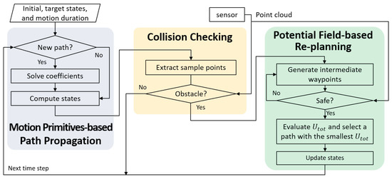
Figure 1.
A flowchart of the overall process proposed.
2.1. Path Propagation Using Motion Primitives
To control differentially flat dynamical systems, such as quadcopters [35], a widely used trajectory planning method is the MPs [31,32]. The MPs are defined by a UAV’s initial state, the desired motion duration, and any combination of components of its position, velocity, and acceleration at the motion’s end. Given those states and conditions, the MPs generate smooth trajectories by minimizing a cost function , where and T denote the jerk and a terminal time, respectively. Indeed, the dynamics into three orthogonal inertial axes are assumed to be decoupled, so the generated MPs minimize the cost value for each axis independent of the other axes. In other words,
where represents a per-axis cost. For each axis q, let the state be the scalar components of position, velocity, and acceleration. The control input is the jerk such that
For shorthand notations, it neglects axis subscript q when only a single axis is considered and time argument , when it is not ambiguous.
The control input jerk is chosen to minimize objective functional in Equation (1). Hamiltonian function is constructed by introducing the time-varying Lagrange multiplier vector , whose elements are called the costates of the system as follows:
The Pontryagin’s minimum principle [36] states that optimal state trajectory , optimal control , and corresponding Lagrange multiplier vector minimize so that the following costate equation must be satisfied:
where represent the gradient of with respect to . Integrating the costate differential equation in Equation (4) with constants , and yields
From Equation (3), is solved by
and is obtained by integrating Equation (2) given the initial condition as follows:
One solves remaining unknowns and depending on the given components of the desired end translational state. As an illustration, when fully defined end translational state is given, let end condition be along an axis. Substituting into Equation (7) and reordering the equation yields
Then, the unknown coefficients and are solved by the inverse of Equation (8) as follows:
Hence, generating the MPs requires only evaluating the matrix multiplication for each axis from Equation (9), and then the state trajectory along the MPs is obtained by Equation (7). In implementation, T in Equation (9) is computed with the desired average speed as follows:
where and represent the initial and target position vector, respectively. For the details of other end conditions, see the Reference [32].
Since the MPs solve for a locally optimal trajectory with respect to allocated time, the trajectory represents time-parameterized polynomials. That is, the closed-form solution of the MPs converts the trajectory generation problem to a problem of finding polynomial coefficients. Thus, the MPs make it possible for the rapid generation and the frequent updates of paths.
2.2. Collision Check Using k-d Tree Search
To navigate in unknown environments, one requirement is real-time sensing of surroundings by remote sensors such as 3D scanners, light detection and ranging (LiDAR) sensors, time-of-flight cameras, and depth sensors. Such sensors measure many points on the external surfaces of objects around them, and the set of those data points is called a point cloud. In other words, since the sensor observes the relative distances between the outer surfaces of the objects and the sensor, the point cloud includes all distance vectors with respect to the center of the sensor, expressed in the sensor reference frame. In fact, depending on computational availability, downsampling the point cloud is sometimes beneficial. In addition, when navigating in dynamic environments, prior mapping is meaningless. Although graph-search algorithms like A* that require map information beforehand need an additional technique or process to deal with dynamic obstacles [37], the proposed approach does not need any additional mapping process, and the updated point cloud, whenever new information becomes available, is useful to represent real-time obstacles.
When the MPs-based motion planning in Section 2.1 are ready for collision checking, an autonomous UAV first extracts sample points from the planned path within the observable area (e.g., sensing range and limited field-of-view (FOV)), shown in Figure 2. Indeed, the maximum distance between two consecutive samples does not exceed the resolution of the point cloud.
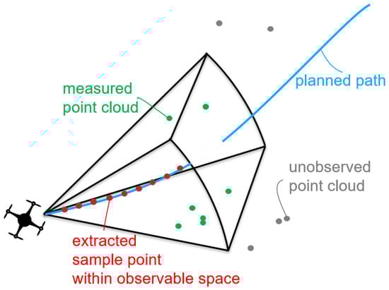
Figure 2.
Sensor’s range and field-of-view (FOV) on the measured point cloud and the extracted sample points.
Next, the k-d tree search algorithm [34] aims to find the nearest obstacle point to each extracted sample-path point. If all closest obstacle points exist outside a certain margin (e.g., collision risk sphere) of the corresponding sample points, then the planned path is assumed to be safe, so the vehicle continues to follow the trajectory. In other words, if the nearest obstacle point exists within the collision risk sphere centered at the corresponding point on the path, re-planning to avoid that path point, called , is performed at the next step in Section 2.3. As a corner case, if is the current location (e.g., when an obstacle moves towards the UAV), then the UAV stops the mission and lands autonomously.
2.3. Re-Planned Path Using Potential Fields
2.3.1. Path Candidates
From the collision checking process, a possible collision risk point along the path is determined. For re-planning on it, one first imagines a tunnel or corridor with a certain radius the UAV has to avoid, centered around . Around that point, the autonomous UAV lists the intermediate waypoint candidates onto the tunnel surface as follows:
where perturbation for asymmetry. The origin of the perpendicular plane is and the normal vector of the plane is the desired velocity at the origin . The vertical vector is a unit vector direction to z-axis in the body frame and the y-axis unit vector follows the right-hand rule , shown in Figure 3. Here, the number of intermediate destinations (i.e., m) enable variability depending on the availability of computing power.
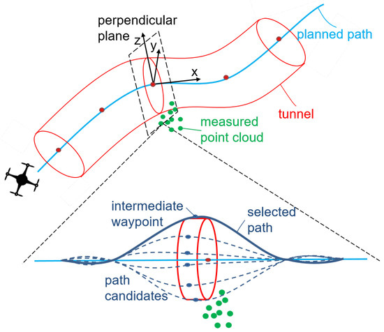
Figure 3.
Perpendicular plane and normal vector on tunnel or corridor and a enlarged figure to illustrate how to generate path candidates.
Next, the MPs create two distinct path segments with a midpoint candidate: one connects from the current position to the intermediate point and the other from the intermediate point to the final location. To smoothly connect the two path segments at that midpoint, in implementation, the following full states at the l-th intermediate point are commonly used as each end condition:
where and
Among m route candidates, unsafe intermediate waypoints are rejected by performing the collision checking process again. If all of the path candidates are unsafe, the UAV sets additional route candidates on the surface of another tunnel with a larger radius at the same sample point for bigger detouring and performs the collision checking of new ones.
2.3.2. Selection of Re-Planned Path Candidates
After rejecting unsafe route candidates, one applies the APF for selecting the best route among the remaining safe-path candidates. In other words, the APF is used for a decision-making purpose here. The APF artificially generates the attractive and repulsive potential fields based on the potential functions by considering the goal, which is the target position, and obstacles. While a UAV is attracted by a goal in the attractive potential field, the UAV is repelled by obstacles in the repulsive potential field. Then, the UAV in a given space travels in a direction where the total potential function value has the minimum value. The total potential function for the safe-path candidates is defined as follows [7]:
where and are the attractive and repulsive potential functions that are defined as
where and are scaling factors for the attractive and repulsive potential functions, is the relative distance between arbitrary two vectors and , is the position vector of measured i-th obstacle, and is the threshold distance influenced by the repulsive potential function. With the the concept of the APF, the -th path that has the smallest total potential function value among the computed values for each path candidate is finally selected as follows:
At the next time step, the above processes are repeated until the UAV arrives at the final goal position.
3. Results
3.1. Urban Modeling
To test CA algorithms in more realistic simulation environments, unlike Lee et al. [33], one models an urban environment with real datasets. In other words, one processes the following steps to generate static obstacles using a city model [38]. The first step is collecting urban data from airborne LiDAR sensors and down-selecting the collected data. The open-source urban information is available at numerous sources. Here, a “.las” file downloaded from Open-Topography (https://opentopography.org/, accessed on 30 March 2021) is utilized, and San Diego downtown is selected as an example of urban environments. Next, one classifies data in the file as the x, y, and z components of a point cloud and filters out only data with a height of z between 200 and 400 ft. For visualization, its scatter plot is depicted in Figure 4. The density of the point cloud is quite similar to the resolution of real-time measurements, so they are sufficient static obstacles in simulations to test CA approaches.
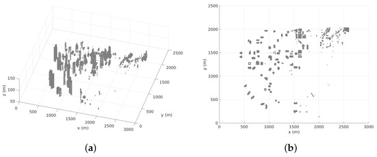
Figure 4.
An example city of urban modeling (a) 3D (b) 2D.
3.2. Simulation Cases and Results
For validating the performance of the proposed approach, one simulates five meaningful scenarios in realistic environments as follows: (i) local minima problem, (ii) GNRON problem, (iii) only static obstacles, (iv) only dynamic obstacles, and (v) complex environment. The first and second cases describe the well-known two major issues of the path planning problems including the APF. The third case tests a 3D environment that contains urban structures as static obstacles, demonstrated in Section 3.1. In the fourth case, a UAV senses other non-cooperative UAVs that are considered as dynamic obstacles. The last challenging case is a complex environment with multiple UAVs (i.e., moving obstacles) in the presence of static obstacles. All of these scenarios are popular in the field of path planning.
In this work, for simulating practical sensing, a range sensor mounted a UAV obtains a point cloud within the measurable space (Figure 2) based on the sensor’s specification. The point cloud includes relative distance information between the UAV and obstacles. In addition, for navigating safely, it assumes that collision occurs when obstacles are inside the risk sphere with a radius of 5 m, centered at the UAV. Here, one assumes no collision at the initial state and no existence of estimation errors and sensing errors. In the processes of the proposed approach, the number of intermediate waypoint candidates is multiples of 8 so that each one is distributed about every 45 deg on the perpendicular plane of the UAV’s path direction. Table 2 lists simulation parameters, and the start and goal positions for each case are tabulated in Table 3. Note that each component of the column vectors represents x, y, and z (altitude), respectively. The following results from the proposed approach are compared to those from the existing APF method.
Table 2.
Simulation parameters.
Table 3.
Start and goal positions of unmanned aerial vehicles (UAVs) for each case.
In case 1, a point of the static obstacle is exactly on the line connecting the start and goal positions. In that environment, the APF yields the UAV gets stuck in the local minima, so the UAV cannot go further avoiding the obstacle as shown in the blue dotted line of Figure 5. In the bird’s eye view, green and pink dots represent the start and goal locations, respectively. Figure 6 depicts the fact that the APF-based UAV (i.e., blue line) stays near the obstacle while maneuvering back and forth around . In the figure, relative distances to the nearest obstacle are measured only within the sensor range (i.e., black dotted line), and both paths do not collide since they are no closer than the collision risk distance (i.e., pink dotted line). In addition, since the heading direction (i.e., sign of the APF’s velocity vector) changes instantaneously as shown in the middle one of Figure 7b, the planned path is dynamically infeasible. However, the proposed approach generates the collision-free path resolving the local minima problem. That is, the proposed method completes the mission within around 82 seconds but the APF cannot since it stays in the local minima area forever (see Figure 7). The red stars illustrated in Figure 5 represent obstacle points that influence re-planning in the approach proposed. With minimal obstacle points (i.e., red stars), a smooth and dynamically feasible trajectory is created, shown in the position vector of Figure 7a.
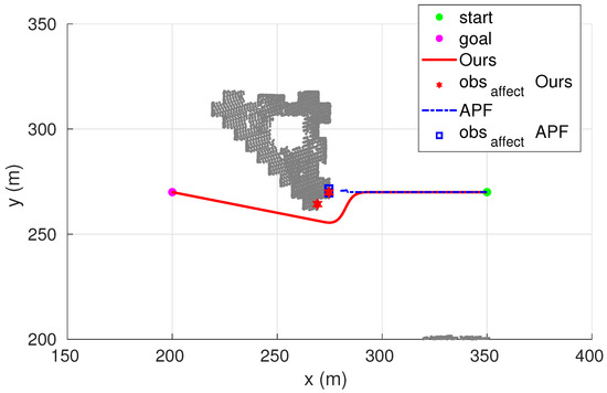
Figure 5.
Bird’s eye view of the local minima problem case.
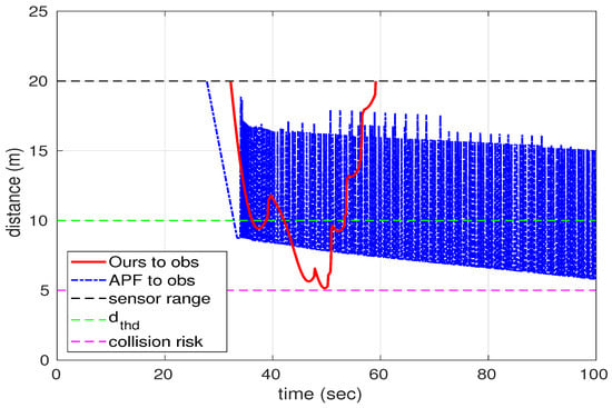
Figure 6.
Relative distance to the nearest obstacle in the local minima problem case.
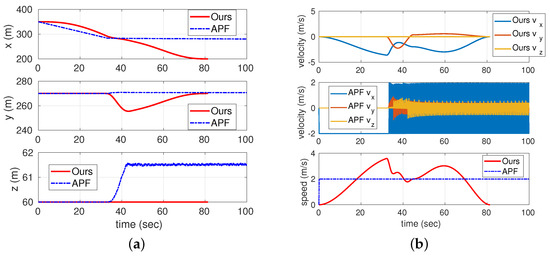
Figure 7.
Translation of the local minima problem case (a) Position (b) Linear velocity and speed.
In case 2, the goal location is set close to 6 m from the static obstacle (pink dot in Figure 8). Like the local minima problem in case 1, such a GNRON environment produces similar results. The APF prevents the UAV from reaching the goal position under the influence of the repulsive potential field. Whereas the APF method keeps the UAV near the region where the repulsive force is affected (see the blue and green lines of Figure 9), the proposed approach enables the UAV to arrive at the destination successfully and safely as exhibited in Figure 8 and Figure 10. Moreover, in the proposed method combining the MPs and APF, the relative distance to the nearest obstacle continues to decrease rapidly, shown in the red line of Figure 9. That is, the UAV based on the proposed approach reaches smoothly the goal location near the obstacle so that the simulation is done within about 45 seconds. However, the UAV based on the APF keeps moving back and forth around the GNRON region, so its final location does not change much (Figure 9 and Figure 10).
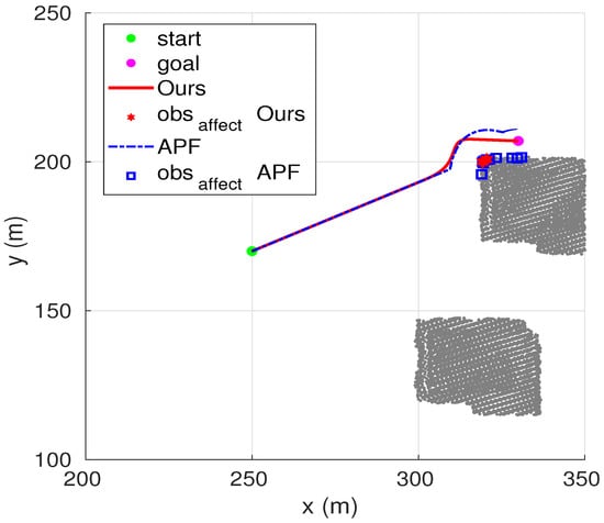
Figure 8.
Bird’s eye view of the goal non-reachable with obstacles nearby (GNRON) problem case.
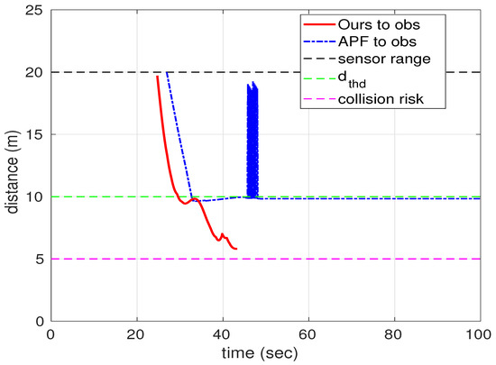
Figure 9.
Relative distance to the nearest obstacle in the GNRON problem case.
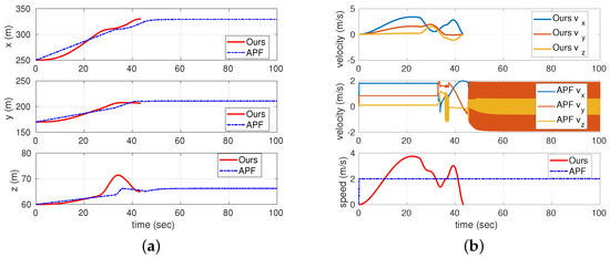
Figure 10.
Translation of the GNRON problem case (a) Position (b) Linear velocity and speed.
The next case is static obstacles only. Figure 11 and Figure 12 highlight the performance of the proposed approach, which provides smooth and continuous position and velocity trajectories. Both methods reach their destination without invading the 5 m collision risk radius as shown in Figure 13, but the APF method is shown to be inefficient since it is affected by more obstacle points and required re-plans more often (i.e., the number of blue squares in Figure 11) than the proposed method experienced (i.e., the number of red stars in Figure 11). Moreover, the APF plans the dynamically impracticable velocity profile enough to require infinite acceleration as shown in the middle one of Figure 12b. In other words, like the proposed approach, the continuous change of the velocity profile is possible dynamically, but like the APF, the relatively discrete variation of the velocity profile is not dynamically executable.
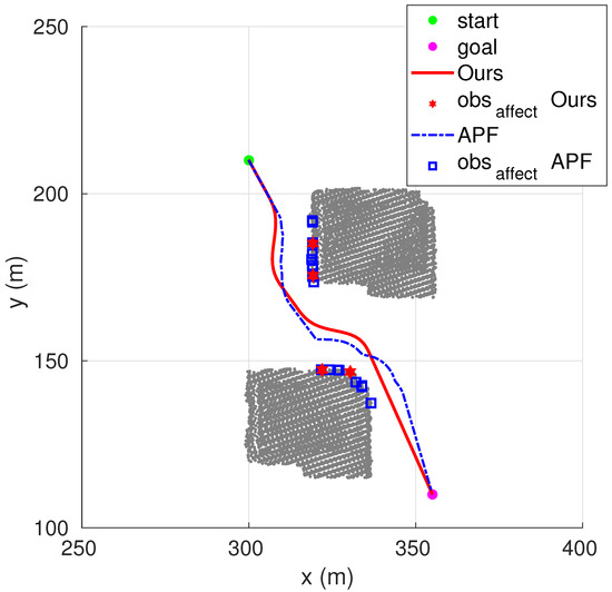
Figure 11.
Bird’s eye view of the static obstacles only case.
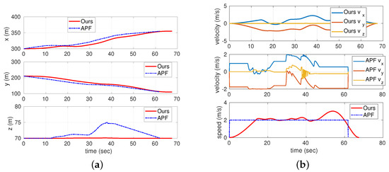
Figure 12.
Translation of the static obstacles only case (a) Position (b) Linear velocity and speed.
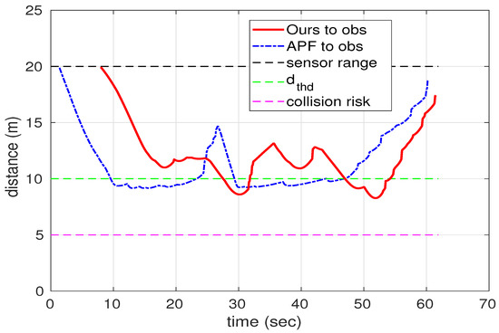
Figure 13.
Relative distance to the nearest obstacle in the static obstacles only case.
In case 4, three UAVs’ starting points (green dots) and destinations (pink dots) are set as if they meet each other around the middle area in the open space (see Figure 14). Here, each UAV is a decentralized agent without any communication like automatic dependent surveillance-broadcast. That is, one UAV does not know the location of the other two UAVs via communication in advance, and like moving obstacles, it can instead predict their rough locations only through real-time measurements of the point cloud. For arrival to the destinations, the APF method becomes inefficient and more dangerous next time since all UAVs are required to do CA too frequently (i.e., the number of blue squares in Figure 14), which results in the repeats of infeasible movement forward and backward (i.e., blue dashed lines in Figure 15, subfigures at the middle row of Figure 16, and blue lines in Figure 17). However, in the proposed method, while UAV2 and UAV3 remain along the initially planned optimal route, only UAV1 efficiently maneuvers a single avoidance whenever the other agents are detected (i.e., red lines in Figure 14 and Figure 15).
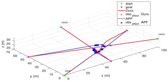
Figure 14.
3D view of the dynamic obstacles only case.
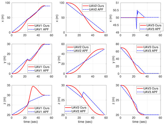
Figure 15.
Positions of each UAV in the case of only dynamic obstacles.
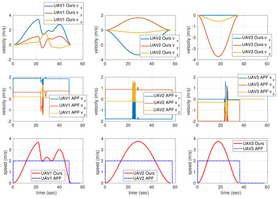
Figure 16.
Linear velocities and speeds of each UAV in the case of only dynamic obstacles.
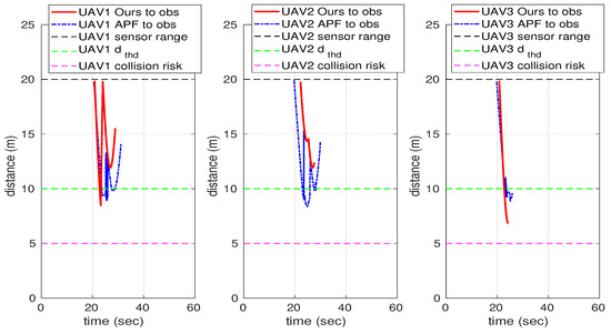
Figure 17.
Relative distance to the nearest obstacle in the case of only dynamic obstacles.
The last scenario is a complex case formed with two moving UAVs and multiple static obstacles. Although both approaches allow all UAVs to reach their goal positions without any collision, similar to case 4, only the proposed method plans optimal (i.e., shorter) and practicable smooth trajectories, shown in Figure 18 and Figure 19. In fact, the proposed method’s UAV2 avoids dynamic (i.e., UAV1) and static obstacles safely during its mission while the proposed method’s UAV1 continues to go along its initially planned path without any collisions. In other words, Figure 18 and Figure 20 show that the APF’s UAV1 has a longer history since it is hindered by UAV2. At similar times, the APF-based UAVs try to avoid each other, so their paths are not planned to be dynamically feasible (i.e., subfigures at the middle row of Figure 21).
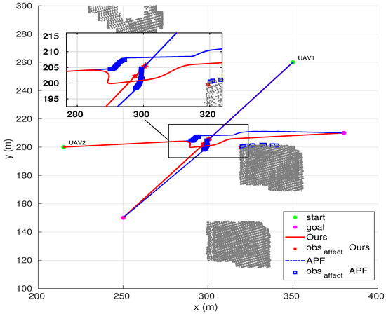
Figure 18.
Bird’s eye view of the complex environment case.
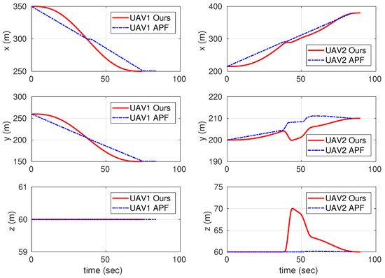
Figure 19.
Position of the complex environment case.
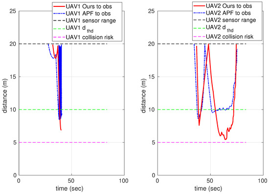
Figure 20.
Relative distance to the nearest obstacle in the complex environment case.
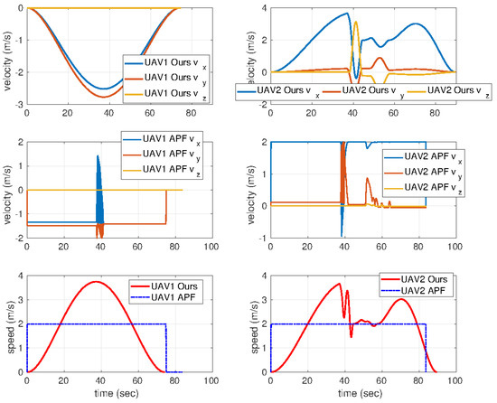
Figure 21.
Linear velocity and speed of the complex environment case.
4. Conclusions
This paper proposes a collision-avoidance approach that combines the artificial potential field (APF) and motion primitives (MPs). Initially, the MPs generate a dynamically feasible and locally optimal trajectory with respect to the allocated time and given states. When collision risk in the planned trajectory is detected by a collision checker, several path candidates around the possible collision risk point are generated for re-planning. After unsafe candidates are rejected, the best route among the remaining safe-path candidates is selected by utilizing the APF. The performance of the proposed approach is validated by numerical simulations with several different scenarios. The unmanned aerial vehicles (UAVs) using the proposed approach reach the goal position along a dynamically feasible trajectory while avoiding collision and the local minima. A practical application of the proposed approach would be the smart mobility corridor for the air traffic management of multiple UAVs’ flights within a complex urban area in the future.
Author Contributions
Conceptualization, K.L.; methodology, K.L.; software, K.L. and D.C.; validation, K.L., D.C., and D.K.; formal analysis, K.L., D.C., and D.K.; investigation, K.L., D.C., and D.K.; resources, K.L. and D.C.; data curation, K.L. and D.C.; writing—original draft preparation, K.L. and D.C.; writing—review and editing, D.K.; visualization, K.L. and D.C.; supervision, D.K.; project administration, D.K.; funding acquisition, D.K. All authors have read and agreed to the published version of the manuscript.
Funding
This research was supported by the research launch award fund at the Office of Research, the University of Cincinnati.
Conflicts of Interest
The authors declare no conflict of interest.
References
- Yu, X.; Zhang, Y. Sense and avoid technologies with applications to unmanned aircraft systems: Review and prospects. Prog. Aerosp. Sci. 2015, 74, 152–166. [Google Scholar] [CrossRef]
- Yasin, J.N.; Mohamed, S.A.; Haghbayan, M.H.; Heikkonen, J.; Tenhunen, H.; Plosila, J. Unmanned aerial vehicles (uavs): Collision avoidance systems and approaches. IEEE Access 2020, 8, 105139–105155. [Google Scholar] [CrossRef]
- Sanchez-Lopez, J.L.; Wang, M.; Olivares-Mendez, M.A.; Molina, M.; Voos, H. A Real-Time 3D Path Planning Solution for Collision-Free Navigation of Multirotor Aerial Robots in Dynamic Environments. J. Intell. Robot. Syst. 2019, 33–53. [Google Scholar] [CrossRef]
- Naderi, K.; Rajamäki, J.; Hämäläinen, P. RT-RRT*: A Real-Time Path Planning Algorithm Based on RRT*. In Proceedings of the 8th ACM SIGGRAPH Conference on Motion in Games, Association for Computing Machinery (MIG’15), Paris, France, 17–18 November 2015; pp. 113–118. [Google Scholar] [CrossRef]
- Mehdi, S.B.; Choe, R.; Hovakimyan, N. Piecewise Bézier Curves for Avoiding Collisions During Multivehicle Coordinated Missions. J. Guid. Control. Dyn. 2017, 40, 1567–1578. [Google Scholar] [CrossRef]
- Zhang, X.; Liniger, A.; Borrelli, F. Optimization-Based Collision Avoidance. IEEE Trans. Control. Syst. Technol. 2020, 1–12. [Google Scholar] [CrossRef]
- Khatib, O. Real-time obstacle avoidance for manipulators and mobile robots. In Proceedings of the 1985 IEEE International Conference on Robotics and Automation, St. Louis, MO, USA, 25–28 March 1985; Volume 2, pp. 500–505. [Google Scholar]
- Wein, R.; Van Den Berg, J.; Halperin, D. Planning high-quality paths and corridors amidst obstacles. Int. J. Robot. Res. 2008, 27, 1213–1231. [Google Scholar] [CrossRef]
- Warren, C.W. Global path planning using artificial potential fields. In Proceedings of the 1989 International Conference on Robotics and Automation, Scottsdale, AZ, USA, 14–19 May 1989; pp. 316–321. [Google Scholar]
- Adeli, H.; Tabrizi, M.; Mazloomian, A.; Hajipour, E.; Jahed, M. Path planning for mobile robots using iterative artificial potential field method. Int. J. Comput. Sci. Issues (IJCSI) 2011, 8, 28. [Google Scholar]
- Li, G.; Tamura, Y.; Yamashita, A.; Asama, H. Effective improved artificial potential field-based regression search method for autonomous mobile robot path planning. Int. J. Mechatron. Autom. 2013, 3, 141–170. [Google Scholar] [CrossRef]
- Choi, D.; Lee, K.; Kim, D. Enhanced Potential Field-Based Collision Avoidance for Unmanned Aerial Vehicles in a Dynamic Environment. In Proceedings of the AIAA Scitech 2020 Forum, Orlando, FL, USA, 6–10 January 2020; pp. 1–7. Available online: https://arc.aiaa.org/doi/pdf/10.2514/6.2020-0487 (accessed on 30 March 2021).
- Bhattacharya, P.; Gavrilova, M.L. Roadmap-based path planning-using the voronoi diagram for a clearance-based shortest path. IEEE Robot. Autom. Mag. 2008, 15, 58–66. [Google Scholar] [CrossRef]
- Gue, J.; Gao, Y.; Cui, G. Path planning of mobile robot based on improved potential field. Inf. Technol. J. 2013, 12, 2188–2194. [Google Scholar] [CrossRef]
- Azzabi, A.; Nouri, K. An advanced potential field method proposed for mobile robot path planning. Trans. Inst. Meas. Control 2019, 41, 3132–3144. [Google Scholar] [CrossRef]
- Triharminto, H.H.; Wahyunggoro, O.; Adji, T.B.; Cahyadi, A.I.; Ardiyanto, I. A Novel of Repulsive Function on Artificial Potential Field for Robot Path Planning. Int. J. Electr. Comput. Eng. 2016, 6, 3262–3275. [Google Scholar] [CrossRef]
- Sudhakara, P.; Ganapathy, V.; Priyadharshini, B.; Sundaran, K. Obstacle Avoidance and Navigation Planning of a Wheeled Mobile Robot using Amended Artificial Potential Field Method. In Proceedings of the International Conference on Robotics and Smart Manufacturing, Chennai, India, 19–21 July 2018; Volume 133, pp. 998–1004. [Google Scholar] [CrossRef]
- Rezaee, H.; Abdollahi, F. Adaptive artificial potential field approach for obstacle avoidance of unmanned aircrafts. In Proceedings of the 2012 IEEE/ASME International Conference on Advanced Intelligent Mechatronics (AIM), Kaohsiung, Taiwan, 11–14 July 2012; pp. 1–6. [Google Scholar]
- Apoorva; Gautam, R.; Kala, R. Motion planning for a chain of mobile robots using a* and potential field. Robotics 2018, 7, 20. [Google Scholar] [CrossRef]
- Azmi, M.Z.; Ito, T. Artificial potential field with discrete map transformation for feasible indoor path planning. Appl. Sci. 2020, 10, 8987. [Google Scholar] [CrossRef]
- Weerakoon, T.; Ishii, K.; Ali, A.; Nassiraei, F. An Artificial Potential Field Based Mobile Robot Navigation Method to Prevent From Deadlock. J. Artif. Intell. Soft Comput. Res. 2015, 5, 189–203. [Google Scholar] [CrossRef]
- Cho, J.H.; Pae, D.S.; Lim, M.T.; Kang, T.K. A Real-Time Obstacle Avoidance Method for Autonomous Vehicles Using an Obstacle-Dependent Gaussian Potential Field. J. Adv. Transp. 2018, 2018, 5041401. [Google Scholar] [CrossRef]
- Chang, K.; Xia, Y.; Huang, K. UAV formation control design with obstacle avoidance in dynamic three-dimensional environment. SpringerPlus 2016, 5, 1124. [Google Scholar] [CrossRef] [PubMed]
- Sun, J.; Tang, J.; Lao, S. Collision avoidance for cooperative UAVs with optimized artificial potential field algorithm. IEEE Access 2017, 5, 18382–18390. [Google Scholar] [CrossRef]
- Park, J.W.; Kwak, H.J.; Kang, Y.C.; Kim, D.W. Advanced fuzzy potential field method for mobile robot obstacle avoidance. Comput. Intell. Neurosci. 2016, 2016, 6047906. [Google Scholar] [CrossRef]
- Elkilany, B.G.; Abouelsoud, A.; Fathelbab, A.M.; Ishii, H. Potential field method parameters tuning using fuzzy inference system for adaptive formation control of multi-mobile robots. Robotics 2020, 9, 10. [Google Scholar] [CrossRef]
- Ahmed, A.A.; Abed, A.A. Path Planning of Mobile Robot by using Modified Optimized Potential Field Method. Int. J. Comput. Appl. 2015, 113, 6–10. [Google Scholar] [CrossRef][Green Version]
- Li, W.; Yang, C.; Jiang, Y.; Liu, X.; Su, C.Y. Motion planning for omnidirectional wheeled mobile robot by potential field method. J. Adv. Transp. 2017, 2017, 4961383. [Google Scholar] [CrossRef]
- Yan, P.; Yan, Z.; Zheng, H.; Guo, J. Real time robot path planning method based on improved artificial potential field method. In Proceedings of the Chinese Control Conference, Technical Committee on Control Theory, Chinese Association of Automation, Wuhan, China, 25–27 July 2018; pp. 4814–4820. [Google Scholar]
- Iswanto, I.; Ma’arif, A.; Wahyunggoro, O.; Cahyadi, A.I. Artificial Potential Field Algorithm Implementation for Quadrotor Path Planning. Int. J. Adv. Comput. Sci. Appl. 2019, 10, 575–585. [Google Scholar] [CrossRef]
- Donald, B.; Xavier, P.; Canny, J.; Reif, J. Kinodynamic motion planning. J. Acm (JACM) 1993, 40, 1048–1066. [Google Scholar] [CrossRef]
- Mueller, M.W.; Hehn, M.; D’Andrea, R. A computationally efficient motion primitive for quadrocopter trajectory generation. IEEE Trans. Robot. 2015, 31, 1294–1310. [Google Scholar] [CrossRef]
- Lee, K.; Choi, D.; Kim, D. Potential Fields-Aided Motion Planning for Quadcopters in Three-Dimensional Dynamic Environments. In Proceedings of the AIAA Scitech 2021 Forum, Virtual, Nashville, TN, USA, 11–15, 19–21 January 2021; p. 1410. [Google Scholar]
- Rusu, R.B.; Cousins, S. 3d is here: Point cloud library (pcl). In Proceedings of the 2011 IEEE International Conference on Robotics and Automation, Shanghai, China, 9–13 May 2011; pp. 1–4. [Google Scholar]
- Mellinger, D.; Kumar, V. Minimum snap trajectory generation and control for quadrotors. In Proceedings of the 2011 IEEE International Conference on Robotics and Automation, Shanghai, China, 9–13 May 2011; pp. 2520–2525. [Google Scholar]
- Bertsekas, D.P. Dynamic Programming and Optimal Control; Athena Scientific: Belmont, MA, USA, 1995; Volume 1. [Google Scholar]
- Chand, B.N.; Mahalakshmi, P.; Naidu, V. Sense and avoid technology in unmanned aerial vehicles: A review. In Proceedings of the 2017 International Conference on Electrical, Electronics, Communication, Computer, and Optimization Techniques (ICEECCOT), Mysuru, India, 15–16 December 2017; pp. 512–517. [Google Scholar]
- Choi, Y.; Pate, D.; Briceno, S.; Mavris, D.N. Rapid and Automated Urban Modeling Techniques for UAS Applications. In Proceedings of the 2019 International Conference on Unmanned Aircraft Systems (ICUAS), Atlanta, GA, USA, 11–14 June 2019; pp. 838–847. [Google Scholar]


Publisher’s Note: MDPI stays neutral with regard to jurisdictional claims in published maps and institutional affiliations. |
© 2021 by the authors. Licensee MDPI, Basel, Switzerland. This article is an open access article distributed under the terms and conditions of the Creative Commons Attribution (CC BY) license (https://creativecommons.org/licenses/by/4.0/).