
Improved Artificial Potential Field and Dynamic Window Method for Amphibious Robot Fish Path Planning

 ,
,  ,
,
Abstract
1. Introduction
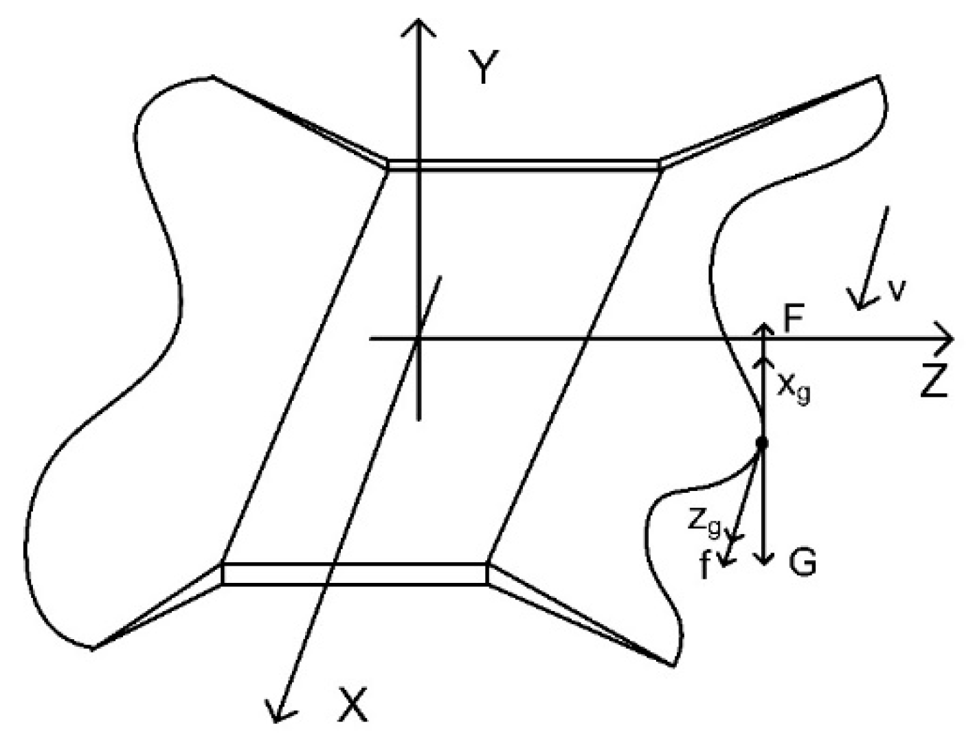
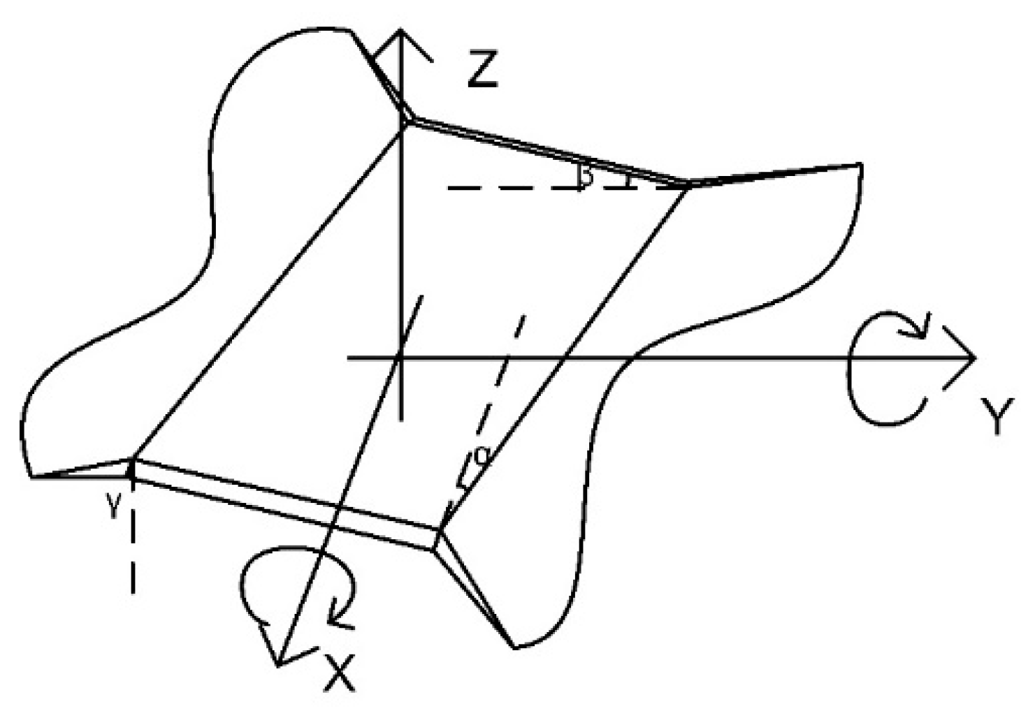
2. Kinetic Analysis
2.1. Kinetic Analysis on the Land
2.2. Kinetic Analysis Underwater
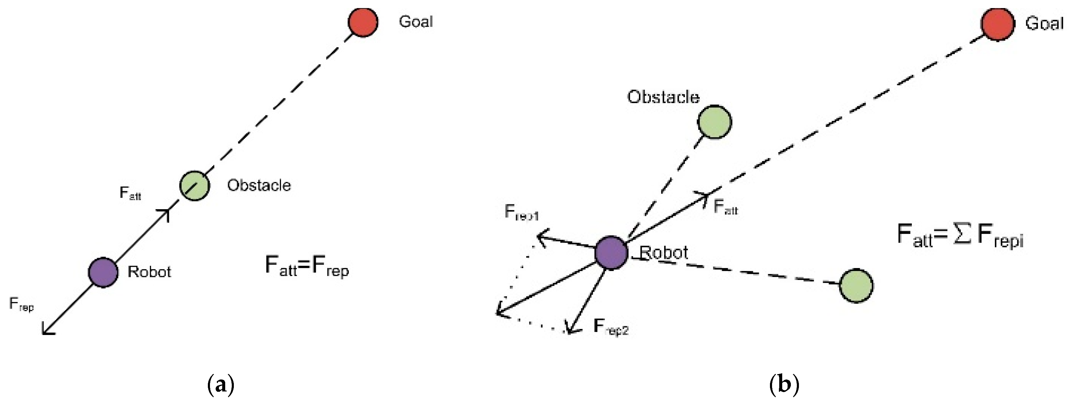
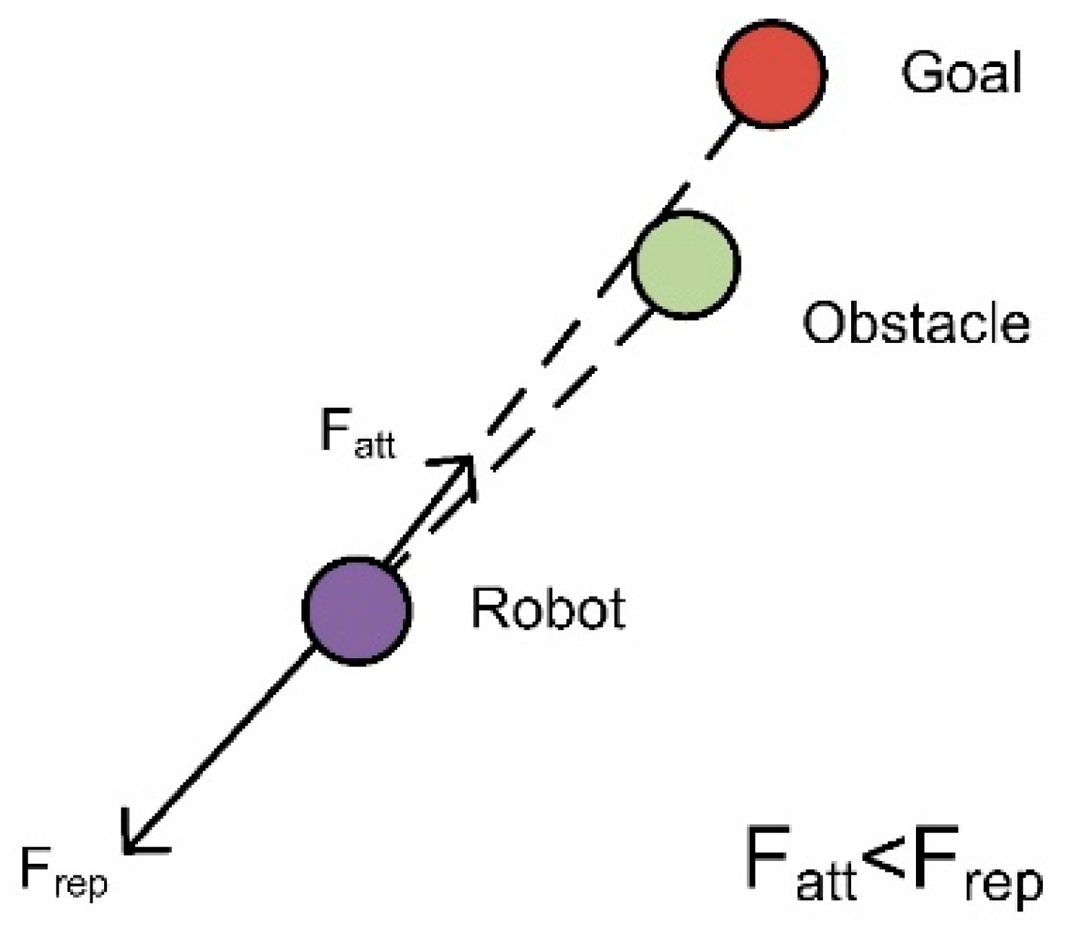
3. Artificial Potential Field Method
3.1. Traditional Artificial Potential Field Method
3.2. Facing Problems
4. Improved Artificial Potential Field Method
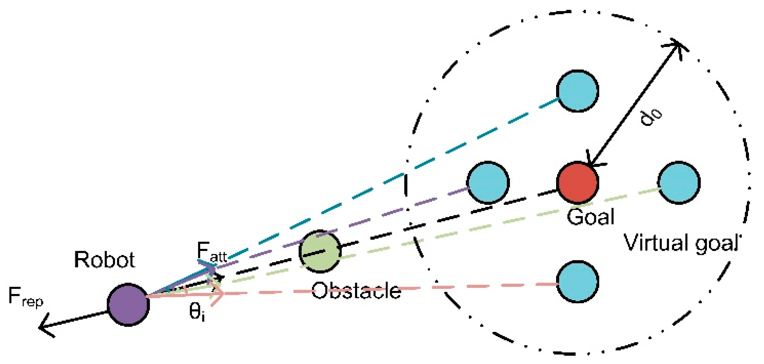
4.1. Improved Attraction Field
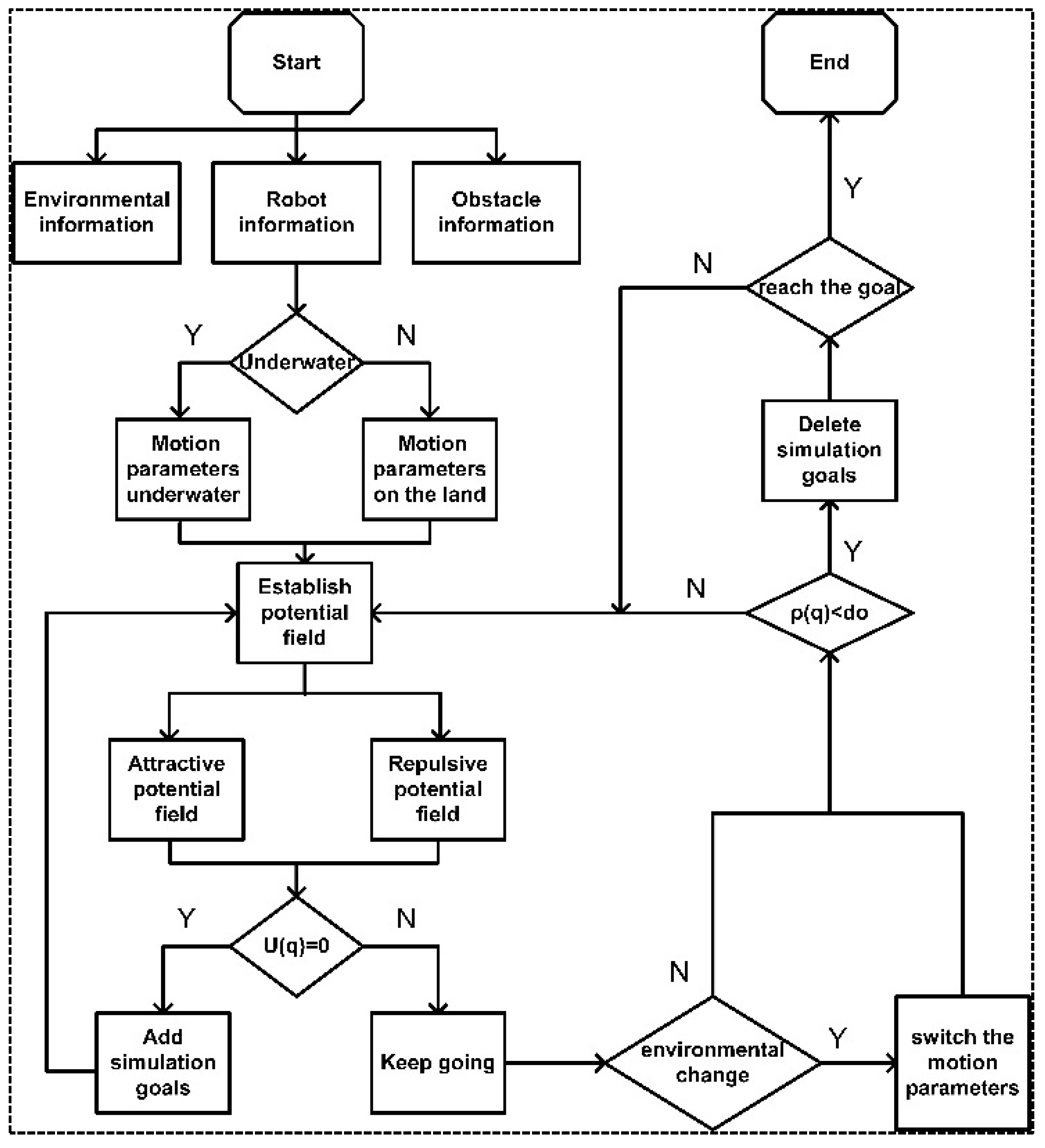
4.2. Combing with Dynamic Window Method
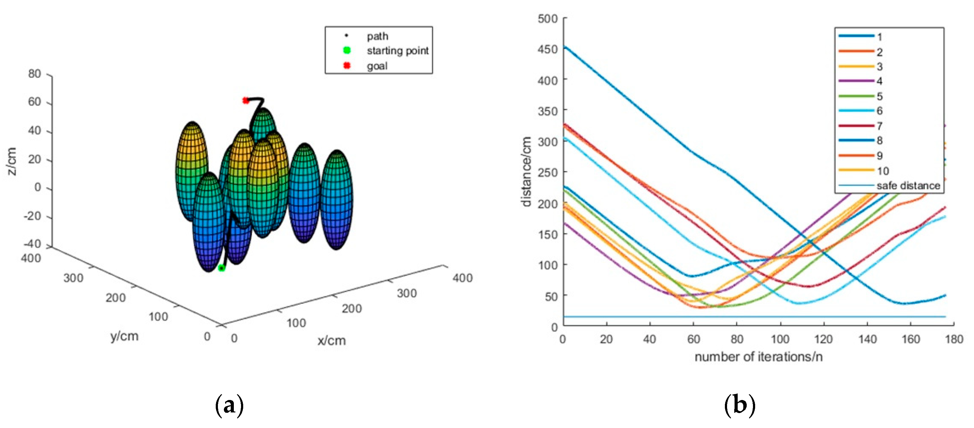
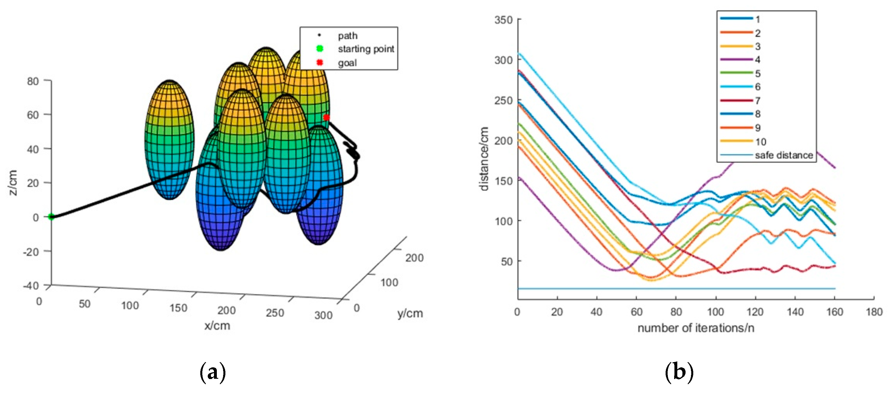
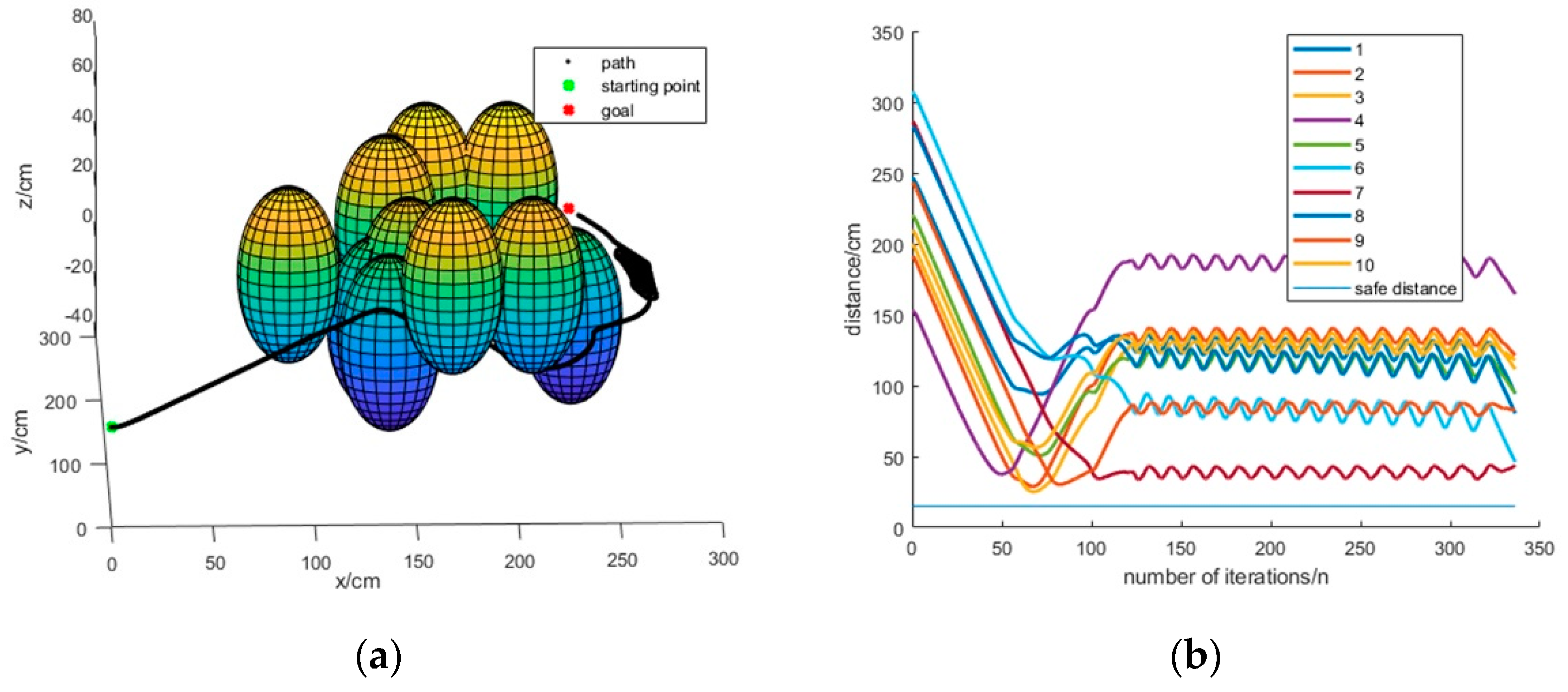
5. Simulation Analysis
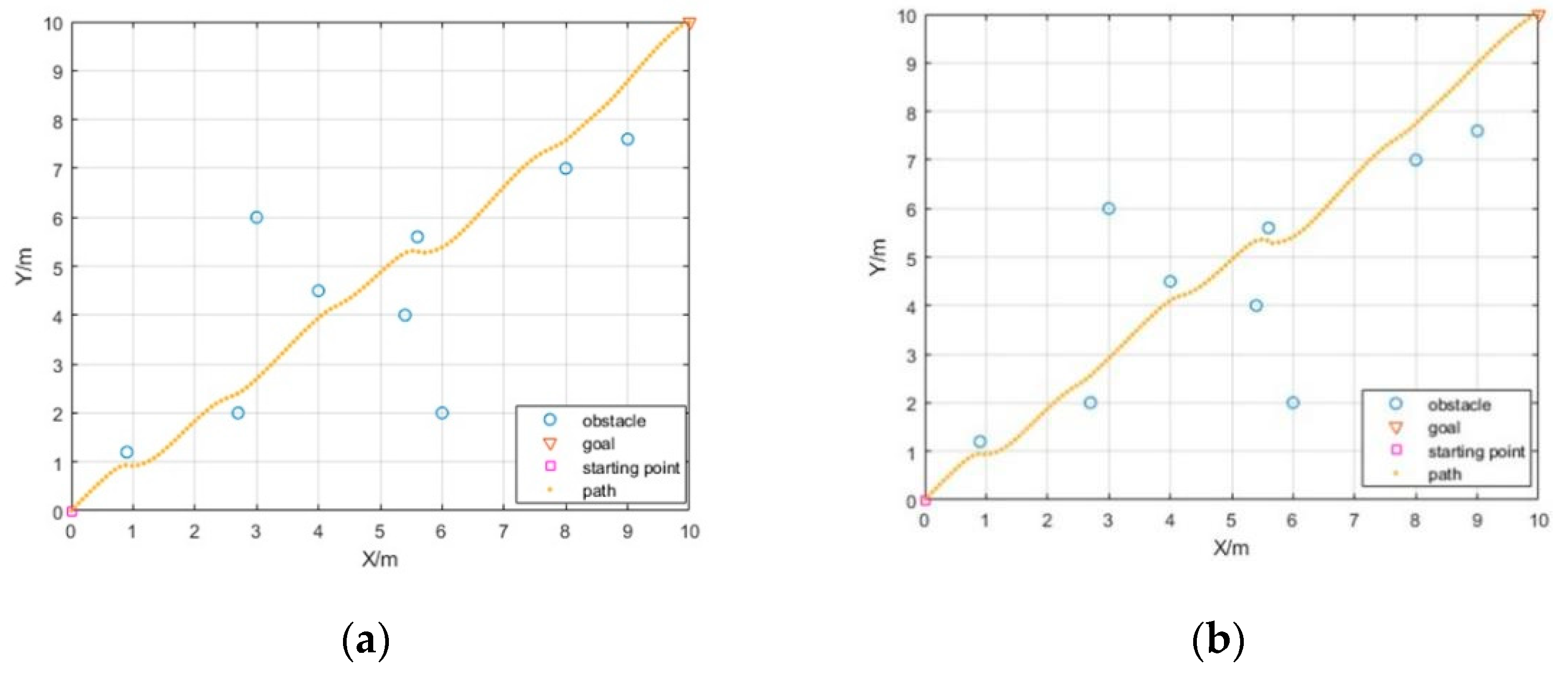
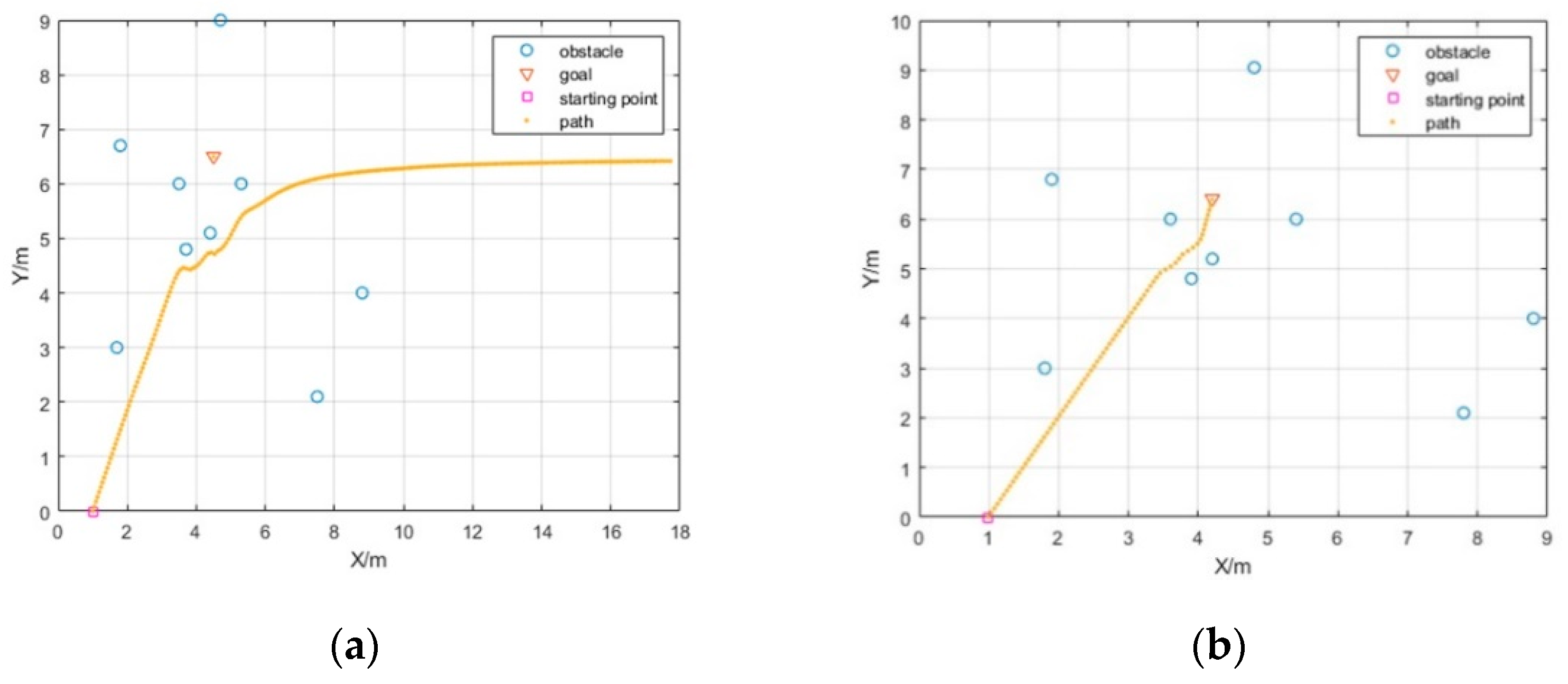
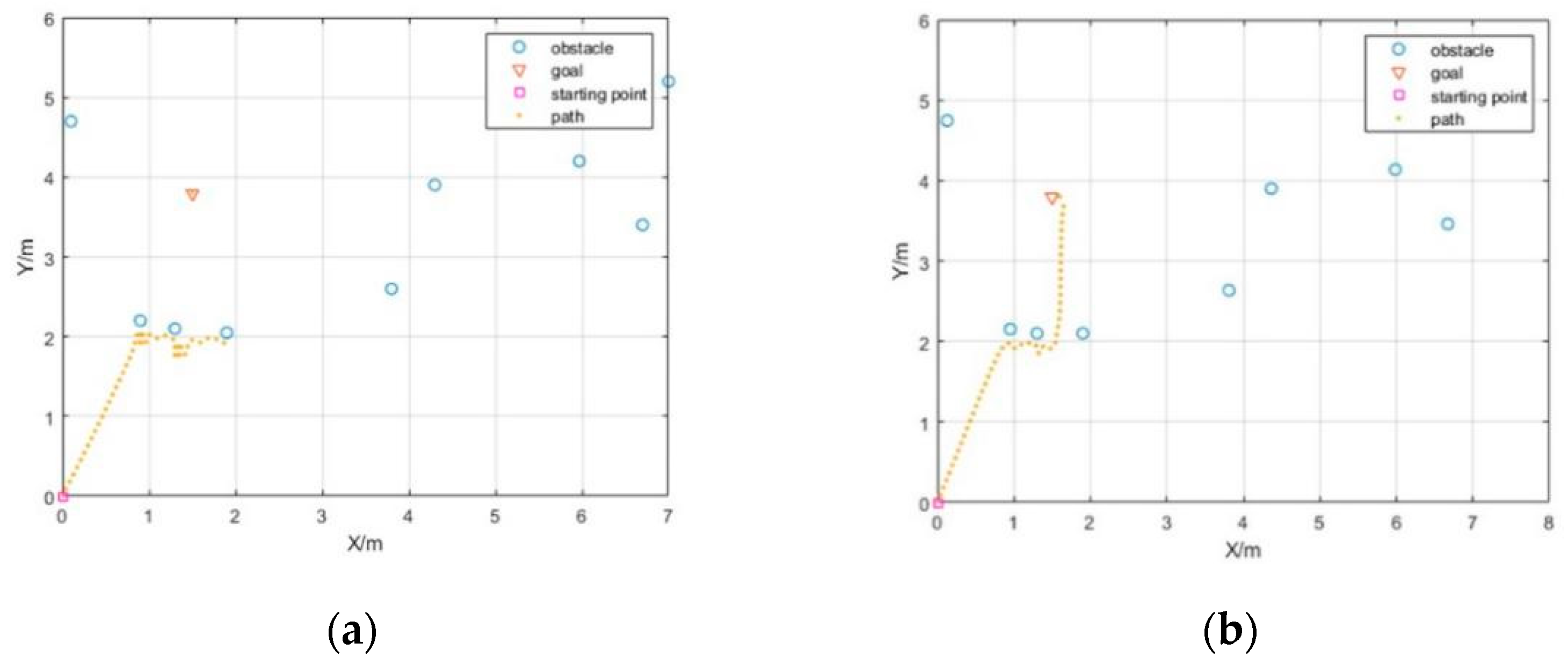
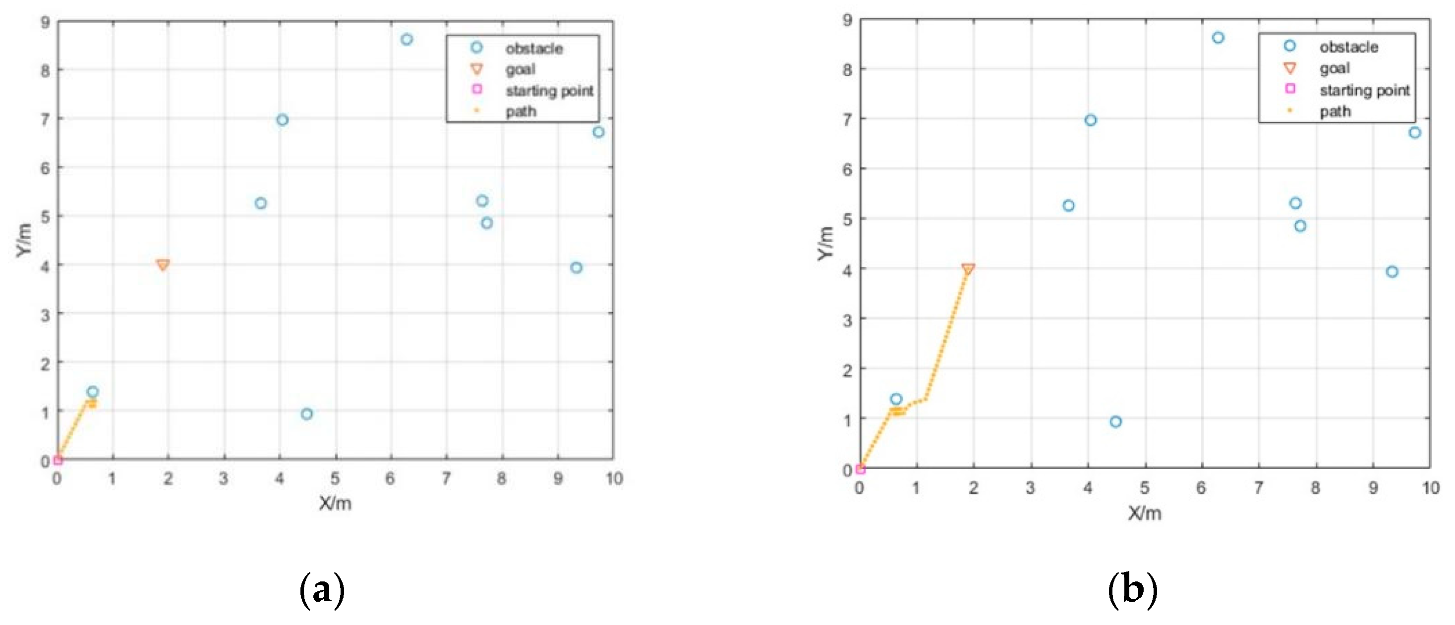
5.1. Simulation of Improved Artificial Potential Field
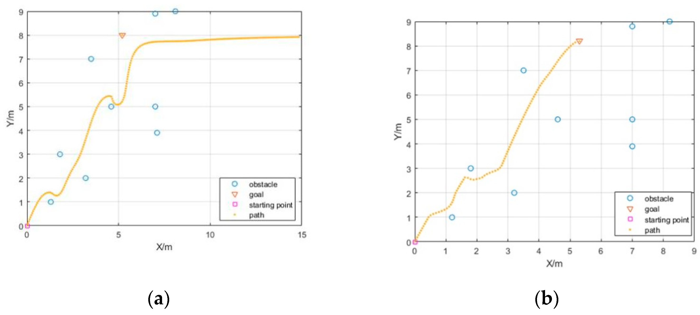
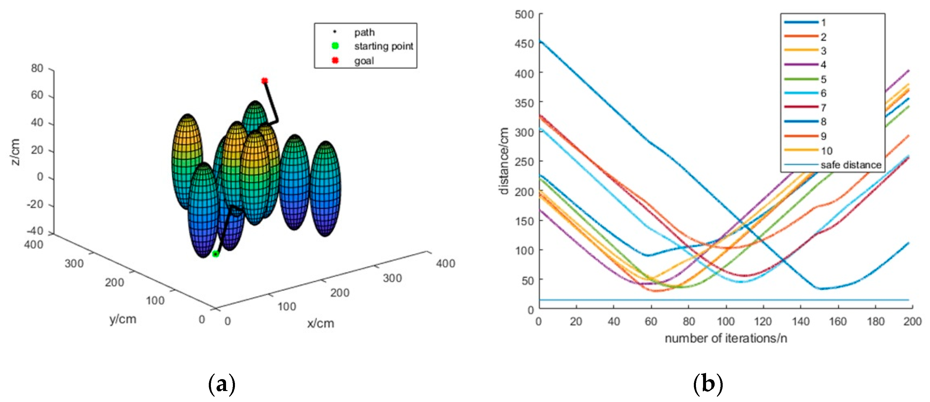
5.2. Simulation of the Hybrid Algorithm
6. Discussion
7. Conclusions
Author Contributions
Funding
Institutional Review Board Statement
Informed Consent Statement
Acknowledgments
Conflicts of Interest
References
- Patle, B.K.; Babu, L.G.; Pandey, A.; Parhi, D.R.K.; Jagadeesh, A. A review: On path planning strategies for navigation of mobile robot. Def. Technol. 2019, 15, 582–606. [Google Scholar] [CrossRef]
- Liu, Y.; Li, Z.; Liu, H.; Kan, Z. Skill transfer learning for autonomous robots and human–robot cooperation: A survey. Robot. Auton. Syst. 2021. [Google Scholar] [CrossRef]
- Pan, M.; Linner, T.; Pan, W.; Cheng, H.-M.; Bock, T. Influencing factors of the future utilization of construction robots for buildings: A Hong Kong perspective. J. Build. Eng. 2021. [Google Scholar] [CrossRef]
- Hawes, N.; Burbridge, C.; Jovan, F.; Kunze, L.; Lacerda, B.; Mudrova, L.; Young, J.; Wyatt, J.L.; Hebesberger, D.; Kortner, T.; et al. The STRANDS Project: Long-Term Autonomy in Everyday Environments. IEEE Robot. Autom. Mag. 2017, 24, 146–156. [Google Scholar] [CrossRef]
- Karami, H.; Hasanzadeh, M. An adaptive genetic algorithm for robot motion planning in 2D complex environments. Comput. Electr. Eng. 2015, 43, 317–329. [Google Scholar] [CrossRef]
- Han, J.; Seo, Y.H. Mobile robot path planning with surrounding point set and path improvement. Appl. Soft Comput. 2017, 57, 35–47. [Google Scholar] [CrossRef]
- Zhang, J.; Xia, Y.; Shen, G. A novel learning-based global path planning algorithm for planetary rovers. Neurocomputing 2019, 361, 69–76. [Google Scholar] [CrossRef]
- Chand, P.; Carnegie, D.A. A two-tiered global path planning strategy for limited memory mobile robots. Robot. Auton. Syst. 2012, 60, 309–321. [Google Scholar] [CrossRef]
- Heinemann, T.; Riedel, O.; Lechler, A. Generating smooth trajectories in local path planning for automated guided vehicles in Production. Proc. Manuf. 2019, 39, 98–105. [Google Scholar] [CrossRef]
- Saranya, K.; Koteswara, R.; Unnikrishnan, M.; Brinda, V.; Lalithambika, V.R.; Dhekane, M.V. Real Time Evaluation of Grid Based Path Planning Algorithms: A comparative study. IFAC Proc. 2014, 47, 766–772. [Google Scholar] [CrossRef]
- Fu, B.; Chen, L.; Zhou, Y.; Zheng, D.; Wei, Z.; Dai, J.; Pan, H. An improved A* algorithm for the industrial robot path planning with high success rate and short length. Robot. Auton. Syst. 2018, 106, 26–37. [Google Scholar] [CrossRef]
- Xie, L.; Xue, S.; Zhang, J.; Zhang, M.; Tian, W.; Haugen, S. A path planning approach based on multi-direction A* algorithm for ships navigating within wind farm waters. Ocean Eng. 2019, 184, 311–322. [Google Scholar] [CrossRef]
- Song, R.; Liu, Y.; Bucknall, R. Smoothed A* algorithm for practical unmanned surface vehicle path planning. Appl. Ocean Res. 2019, 83, 9–20. [Google Scholar] [CrossRef]
- Jiao, Z.; Ma, K.; Rong, Y.; Wang, P.; Zhang, H.; Wang, S. A path planning method using adaptive polymorphic ant colony algorithm for smart wheelchairs. J. Comput. Sci. 2018, 25, 50–57. [Google Scholar] [CrossRef]
- Wang, Z.; Zhu, X.; Han, Q. Mobile robot path planning based on parameter optimization ant colony algorithm. Proc. Eng. 2011, 15, 2738–2741. [Google Scholar]
- Orozcorosas, U.; Montiel, O.; Sepúlveda, R. Mobile robot path planning using membrane evolutionary artificial potential field. Appl. Soft. Comput. 2019, 77, 236–251. [Google Scholar] [CrossRef]
- Keyu, W.; Esfahani, M.A.; Yuan, S.; Wang, H. TDPP-Net: Achieving three-dimensional path planning via a deep neural network architecture. Neurocomputing 2019, 357, 151–162. [Google Scholar]
- Wang, M.; Su, Z.; Tu, D.; Lu, X. A hybrid algorithm based on Artificial Potential Field and BUG for path planning of mobile robot. In Proceedings of the 2013 2nd International Conference on Measurement, Information and Control, Harbin, China, 16–18 August 2013. [Google Scholar]
- Yuan, M.; Wang, S.; Wu, C.; Li, K. Hybrid ant colony and immune network algorithm based on improved APF for optimal motion planning. Robotica 2010, 28, 833–846. [Google Scholar]
- Lee, M.; Park, M.G. Artificial potential field-based path planning for mobile robots using a virtual obstacle concept. In Proceedings of the 2003 IEEE/ASME International Conference on Advanced Intelligent Mechatronics (AIM 2003), Kobe, Japan, 20–24 July 2003. [Google Scholar]
- Wang, Q.; Cheng, J.; Li, X. Path planning of robot based on improved artificial potentional field method. In Proceedings of the 2017 International Conference on Artificial Intelligence, Automation and Control Technologies, Wuhan, China, 7–9 April 2017. [Google Scholar]
- Ballesteros, J.; Urdiales, C.; Velasco, A.B.M.; Ramos-Jiménez, G. A biomimetical dynamic window approach to navigation for collaborative control. IEEE Trans. Hum. Mach. Syst. 2017, 47, 1123–1133. [Google Scholar] [CrossRef]


| Name | Symbol | Underwater | Land |
|---|---|---|---|
| Total mass | 10 kg | 10 kg | |
| Length of the fin surface | 75 cm | 75 cm | |
| Wavelength | 20 cm | 20 cm | |
| Coulomb friction coefficient | / | 0.85 | |
| Velocity | 0.23 m/s | 0.13 m/s | |
| Angular velocity | 0.31 rad/s | 0.12 rad/s |
| Name | Symbol | Value |
|---|---|---|
| Attractive field factor | 15 | |
| Repulsive field factor | 5 | |
| Obstacle influence distance | 1 m | |
| Goal influence range | 3 m | |
| Maximum number of iterations | 200 | |
| Time step | 0.1 s | |
| Angle influence factor | 0.2 | |
| Velocity influence factor | 0.1 | |
| Distance influence factor | γ | 0.1 |
| Method | Figure | Execution time | Path Length |
|---|---|---|---|
| traditional artificial potential field method | 7a | 0.8230 s | 14.1421 m |
| 8a | 0.7760 s | 11.0143 m | |
| 9a | 0.7990 s | 17.8513 m | |
| improved artificial potential field method | 7b | 0.7910 s | 14.1421 m |
| 8b | 0.6930 s | 9.7637 m | |
| 9b | 0.5430 s | 8.9057 m |
| Method | Figure | Execution Time | Path Length |
|---|---|---|---|
| traditional artificial potential field method | 10a | 0.7830 s | 2.6717 m |
| 11a | 0.7770 s | 1.3853 m | |
| improved artificial potential field method | 10b | 0.8030 s | 4.1231 m |
| 11b | 0.7940 s | 4.4283 m |
Publisher’s Note: MDPI stays neutral with regard to jurisdictional claims in published maps and institutional affiliations. |
© 2021 by the authors. Licensee MDPI, Basel, Switzerland. This article is an open access article distributed under the terms and conditions of the Creative Commons Attribution (CC BY) license (http://creativecommons.org/licenses/by/4.0/).
Share and Cite
Yang, W.; Wu, P.; Zhou, X.; Lv, H.; Liu, X.; Zhang, G.; Hou, Z.; Wang, W. Improved Artificial Potential Field and Dynamic Window Method for Amphibious Robot Fish Path Planning. Appl. Sci. 2021, 11, 2114. https://doi.org/10.3390/app11052114
Yang W, Wu P, Zhou X, Lv H, Liu X, Zhang G, Hou Z, Wang W. Improved Artificial Potential Field and Dynamic Window Method for Amphibious Robot Fish Path Planning. Applied Sciences. 2021; 11(5):2114. https://doi.org/10.3390/app11052114
Chicago/Turabian StyleYang, Wenlin, Peng Wu, Xiaoqi Zhou, Haoliang Lv, Xiaokai Liu, Gong Zhang, Zhicheng Hou, and Weijun Wang. 2021. "Improved Artificial Potential Field and Dynamic Window Method for Amphibious Robot Fish Path Planning" Applied Sciences 11, no. 5: 2114. https://doi.org/10.3390/app11052114
APA StyleYang, W., Wu, P., Zhou, X., Lv, H., Liu, X., Zhang, G., Hou, Z., & Wang, W. (2021). Improved Artificial Potential Field and Dynamic Window Method for Amphibious Robot Fish Path Planning. Applied Sciences, 11(5), 2114. https://doi.org/10.3390/app11052114