Self-Supervised Transfer Learning from Natural Images for Sound Classification

Abstract

We propose the implementation of transfer learning from natural images to audio-based images using self-supervised learning schemes. Through self-supervised learning, convolutional neural networks (CNNs) can learn the general representation of natural images without labels. In this study, a convolutional neural network was pre-trained with natural images (ImageNet) via self-supervised learning; subsequently, it was fine-tuned on the target audio samples. Pre-training with the self-supervised learning scheme significantly improved the sound classification performance when validated on the following benchmarks: ESC-50, UrbanSound8k, and GTZAN. The network pre-trained via self-supervised learning achieved a similar level of accuracy as those pre-trained using a supervised method that require labels. Therefore, we demonstrated that transfer learning from natural images contributes to improvements in audio-related tasks, and self-supervised learning with natural images is adequate for pre-training scheme in terms of simplicity and effectiveness.

1. Introduction

Deep learning is neural networks that can learn and analyze the relationship among the data and label inspired by the structure of a human brain. Recently, deep learning has been widely applied in audio-related tasks and achieved superior performance compared to traditional methods [1,2,3,4], especially in real-time smartphone-based voice activity dectection [5], and typing software by recognizing voice [6], sound event classification in noisy environment [7,8], environment sound classification, such as car horn and air conditional sound [9], and speech emotion recognition [10,11,12]. Among the deep learning methods, recurrent neural networks (RNNs) and convolutional neural networks (CNNs) play an important role in audio tasks. RNNs is a network that process sequential inputs by utilizing the output of the before layer as input for the successive layer. It can extract temporal features from the 1-dimensional signals. CNNs is a network that process spatial information by striding the kernels for successive layers. It can extract spatial features from the 2-dimensional images. Yoshimura et al. [13] utilized an RNN to recognize speech from a 1D waveform by extracting temporal information from time-series data. There are some studies utilizing the 2D CNN for the audio related tasks. For the CNN, 1D audio signal is required to be converted into 2D. The spectrogram is one of the visual representation methods that indicates the frequencies of a signal along the time variations. In many studies [5,14], spectrogram representation has been adopted for representing the sound. Sehgal et al. [5] utilized a 2D CNN for speech recognition, which input a 2D spectrogram converted from a 1D waveform. Instead of RNN, the CNN focused more on the spatial features in the spectrogram images. Supervised deep learning-based methods require a large set of labeled data since unsupervised learning does not have that issue.

Although deep learning-based methods perform well on audio-related tasks, they require a large set of labeled data to be appropriately generalized on the test data. To train deep neural networks for new tasks, a large, labeled dataset must be constructed. However, labeling a large set of data is labor intensive especially for the audio data. This drawback has led to the determination of efficient learning schemes, such as transfer learning [15,16]. Transfer learning is a method that utilizes the network pre-trained with largely available dataset on the other relevant tasks. Based on the ImageNet [17], which is the large size image benchmark that consists of 14 million images, transfer learning achieved significant improvements on many image related tasks [18,19]. However, in the audio domain, audio benchmark which has enough number of samples for transfer learning does not available. Instead, Palanisamy et al. [14] proposed to utilize the transfer learning from natural images to audio-based images. They trained the CNN network using the images and corresponding labels of ImageNet and fine-tuned on audio benchmark dataset. By achieving the state-of-the-art results on three benchmarks (ESC-50 [20], GTZAN [21], and UrbanSound8K [22]), they demonstrated that the network pre-trained with massive natural image dataset can be utilized for improving the performance of other domain’s task.

However, transfer learning method proposed by [14] require labels along with the images for pre-training; usually transfer learning is utilized in the cases that the number of labels appropriate for tasks are small; requiring the additional labels for the transfer learning reduce the effectiveness of transfer learning. Additionally, there are extremely large unlabeled image dataset, but they cannot be utilized for the transfer learning that requires labels and only limited to the labeled dataset which has far fewer number of samples compared to the unlabeled ones. To apply the transfer learning across domains (natural images to audio domain), we proposed to utilize the self-supervised learning methods for pre-training instead of supervised ones. Self-supervised learning is a method for learning the general representation of images by learning dissimilarity among the different images and similarity between the ame images without labels [23,24,25,26,27,28]. Therefore, we pre-trained a large number of unlabeled natural images using self-supervised scheme and fine-tuned on audio-based images. Through the experiments on sound classification tasks, we demonstrated that the transfer learning from natural images to audio domain via self-supervised learning scheme can significantly improve the performance with the similar level of supervised ones. In addition, constructing an unlabeled dataset is significantly easier than constructing a labeled dataset. Therefore, self-supervised transfer learning can yield more successful results than supervised learning when a considerably large number of unlabeled images are used.

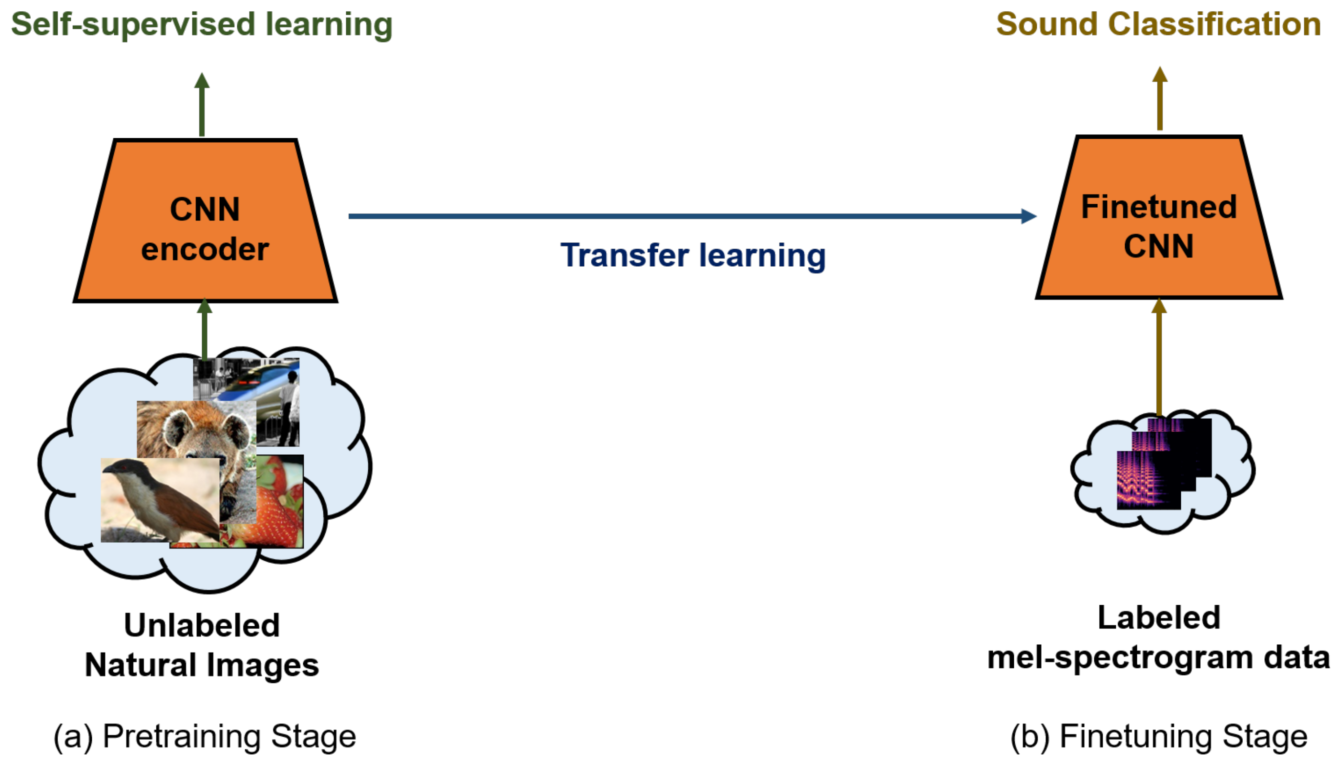
In summary, our proposed training architecture comprises two steps. First, pre-training a CNN with natural images via self-supervised learning. Second, fine-tuning the CNN with labeled 2D-spectrogram audio samples. Our main contributions can be summarized as follows:

• We demonstrated that pre-trained networks with natural images can improve the performance of audio-related tasks with precise pre-training schemes.
• Networks pre-trained through self-supervised learning have similar effects on the performance of audio tasks as those pre-trained through supervised methods.
• When the self-supervised transfer learning scheme was validated using general sound classification datasets, such as (ESC-50, GTZAN, and UrbanSoun8K), the classification accuracy was significantly improved.

We organized the rest of the paper as follows. In the following, Section 2, we introduce the transfer learning and self-supervised learning methods related to our works. In Section 3, we describe the method about pre-processing, self-supervised learning scheme, and our training mechanism with transfer learning and self-supervised learning. Section 4 presents the experimental results validated on the audio benchmarks and provides discussion about the results. Finally, in Section 5, we report the conclusion.

2. Related Works

2.1. Transfer Learning on Natural Image Domain

Transfer learning is a method that utilizes the network pre-trained with largely available dataset as a starting point [15,16]. After the pre-training, the network is trained using the target dataset. This simple method can improve the performance in various cases, especially in image-related tasks. For instance, Tajbakhsh et al. [15] demonstrated that a CNN trained from scratch exhibits significantly inferior performance for medical image analysis compared with that trained from pre-trained networks using ImageNet [17]. Marmanis et al. [16] showed that a fine-tuned network with a small fraction of target samples outperforms networks trained from scratch with all samples. Other studies [18,19] also showed that a pre-trained CNN can improve the discriminativeness of unsupervised image clustering. These results reinforce the concept that CNNs pre-trained on large image datasets can extract well-generalized features and can be transferred to other networks.

2.2. Transfer Learning on Audio Domain

Likewise, some studies used pre-trained CNN models to improve the performance of audio-related tasks [29,30,31]. Choi et al. [29] proposed a transfer learning framework from a network pre-trained for music tagging for general music-related tasks. It utilized the concatenated feature maps of multiple layers in a pre-trained CNN as efficient transferable knowledge and showed that transfer learning using concatenated features improved the performance of various general music-related tasks. Lee et al. [31] proposed music auto-tagging networks that used the aggregated features from pre-trained networks with different shapes and types of audio features. Kong et al. [30] utilized transfer learning by pre-training networks with large-scale audio data and achieved state-of-the-art performance in several audio tasks. This indicates that transfer learning schemes are effective in the audio domain.

However, there is a lack of large-scale public audio datasets for pre-training. Therefore, new paradigms for transfer learning that utilize a network pre-trained with natural images are transferred to audio-related tasks. Palanisamy et al. [14] showed that, even though pre-trained networks are not designed for audio tasks, a fine-tuned network pre-trained with ImageNet [17] can achieve state-of-the-art results in general sound classification tasks. This result demonstrated that knowledge from natural images can help in audio-based spectrogram analysis; moreover, it can be transferred to pre-training schemes.

2.3. Self-Supervised Learning

Pre-training with natural images can improve the performance of audio tasks; thus, we designed transfer learning schemes based on self-supervised learning instead of supervised learning. Through self-supervised learning, the useful representations of images can be learnt without their corresponding labels; this does not require additional human labor for pre-training. Early studies on self-supervised learning relied on heuristic pretext tasks [32,33,34,35]. For example, Zhang et al. [33] proposed a training framework that estimated the two associated color channels of images using the given single-channel images in the CIE lab color space. Noroozi et al. [34] proposed a self-supervised learning method in which the networks were trained to solve jigsaw puzzle-like problems that predicted the manually occluded parts of images. Recently, Gidaris et al. [35] pre-trained networks for predicting the angles of images, which were randomly rotated in advance. Although these studies suggested that pre-training for heuristics pretext tasks can help in learning the general representation of images, their methods require well-defined pretext tasks and do not always work. Recently, contrastive learning-based self-supervised learning demonstrated superior performance in numerous tasks (significantly improved performance compared to previous state-of-the-art methods) [23,24,25,26,27,28]. Contrastive learning that learns the similarity between images were proposed by the siamese network [36] for one shot classification. However, it requires label indicating that whether the given images are the same objects. To utilize the contrastive learning in the self-supervised learning, augmentations was adopted for generating positive samples that denote same-class samples without manually annotated labels. Dosovitskiy et al. [24] proposed an automated self-supervised learning scheme without pretext tasks by training a network to estimate the number of original images from the given augmented images. The network could learn the similarity between samples to count the original images from augmented samples. Bachman et al. [26] developed a self-supervised learning scheme that maximized the mutual information in the features extracted from cropped images from multiple locations of an original image. Recently, Chen et al. [28] proposed semi-supervised learning schemes that used a pre-trained network with self-supervised learning as a teacher and fine-tuned the teacher network using a small fraction of target samples; then, the logit from the fine-tuned teacher network was distilled into the target network using a large number of unlabeled samples and small number of labeled samples. This procedure achieved a top-1 accuracy of 73.9% in ImageNet using only 1% of the labeled ImageNet data [37], while standard supervised ResNet-50 achieved an accuracy of 25.4% under the same conditions. Self-supervised learning can be utilized for pre-training without labels.

3. Method

3.1. Data Pre-Processing

We used a 2D CNN for audio classification; therefore, the 1D waveform was converted into a 2D waveform. Previous studies found that mel-spectrograms are suitable for 2D representation of sound for the benchmarks we used for this study [14]. Therefore, we transformed the audio clips into a mel-spectrogram by applying short-time Fourier transform (STFT) and mel-filters. STFT is a Fourier-related transform used to determine the sine wave frequency and phase content of a local cross-section of a signal across time.

$$STFT\left(x\right)=\sum _{n=0}^{N-1}x\left[n\right]·W\left[t\right]$$

(1)

$$x_{spec}=STFT\left(x_{raw}\right),x_{raw}\in R^{1\times T}.$$

(2)

$x_{raw}$ and $x_{spec}$ denote the 1D raw waveform and 2D spectrogram, respectively. When a raw discrete digital signal is input to STFT function, part of raw signal $x\left[n\right]$ and window function ($W\left[t\right]=e^{(-j2fn)}$) was utilized to calculate spectrum, where t and f indicates time and frequency, respectively. N, which is number of bins for STFT, was set to 4410 for ESC-50, and 2205 for others.

After STFT, mel-filter banks generated by the function of mel-filters ($H_m\left(k\right)$) were applied to extract features from the frequency domain by focusing more on low-frequency regions. Here, $f\left(m\right)$ indicates Hertz function calculated from the mel (m) and the mel-filter banks are the collections of mel-filters for the various k. As illustrated in Figure 1, filters are located in the low-frequency region more densely than the high-frequency regions to emphasize the differences in low-frequency region inspired by the human auditorium system.

$$H_m\left(k\right)=\left\{\begin{array}{cc}0\hfill & k<f(m-1)\hfill \\ \frac{k-f(m-1)}{f\left(m\right)-f(m-1)}\hfill & f(m-1)<k<f\left(m\right)\hfill \\ 1\hfill & k=f\left(m\right)\hfill \\ \frac{f(m+1)-k}{f(m+1)-f\left(m\right)}\hfill & f\left(m\right)<k<f(m+1)\hfill \\ 0\hfill & k>f(m+1)\hfill \end{array}\right.,$$

(3)

$$x_{mel}=H_m\left(k\right)\ast x_{spec},x_{spec}\in R^{F\times T}.$$

(4)

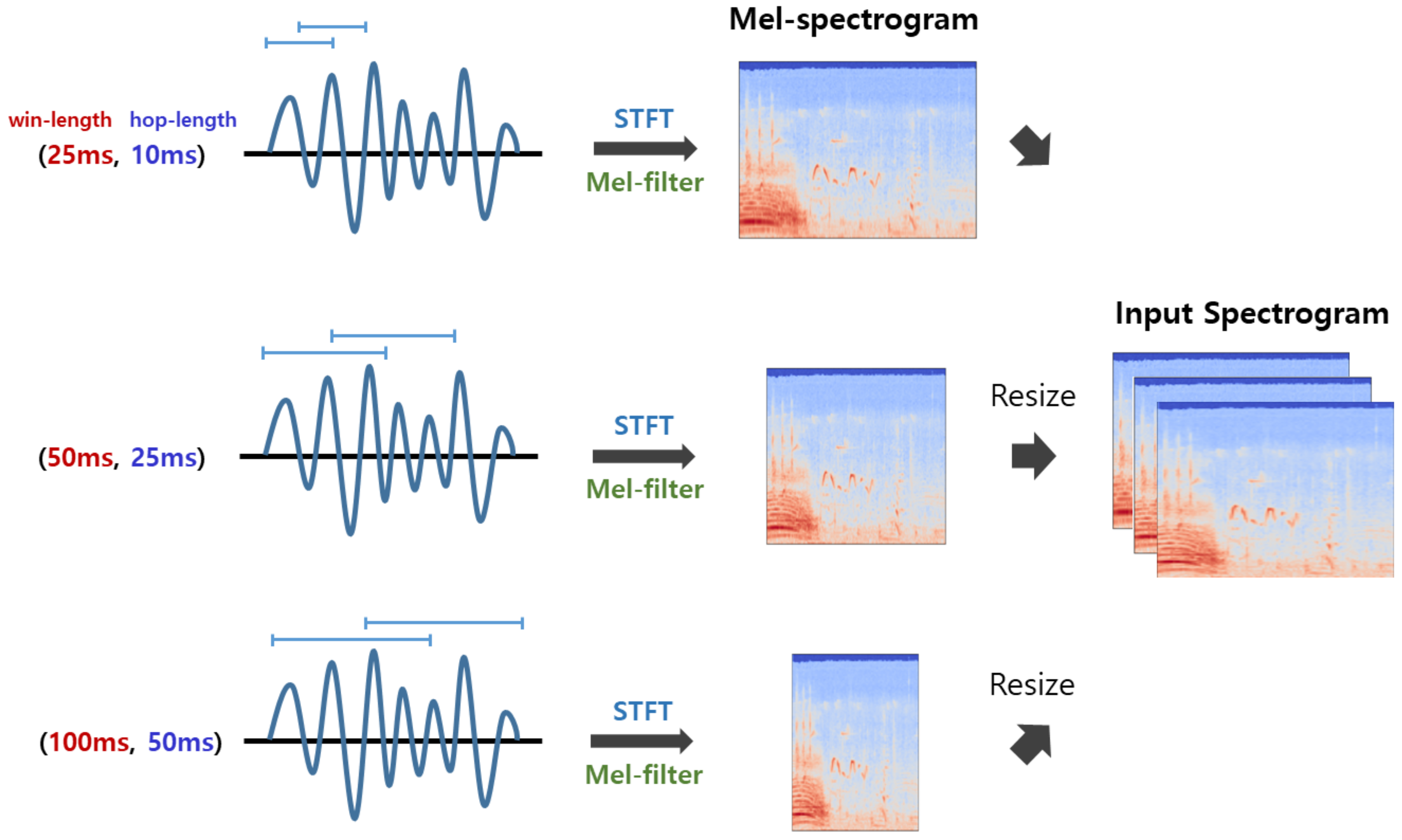
Mel-spectrogram, shown in Figure 2, is generated by passing the input spectrogram into the mel-filters calculated by Equation (4). Here, $x_{mel}$ indicates mel-spectrogram; T and F denote the time scale and number of frequency bins, respectively.

Through mel-spectrogram generation, 1D audio signal expands its dimension into two (time and frequency domain). As a result, spectrogram and mel-spectrogram has single channel in the sense of image dimensions. However, natural images have three channels for each pixel; therefore, spectrogram and mel-spectrogram must be converted into three channels for the transfer learning. As proposed in a previous study [14], we generated three different mel-spectrograms from a single mel-spectrogram by applying three filters with different window sizes and hop lengths into the same signal (Figure 2). For the first, second, and third channels, mel-spectrograms generated with a window size and hop length of 25 and 10 ms, 50 and 10 ms, and 100 and 50 ms, respectively, were used. Owing to the differences in window size and hop length, all mel-spectrograms were of different size. Therefore, all mel-spectrograms were resized into size of the largest one. Subsequently, the mel-spectrogram used in ESC-50 and UrbanSound8k had an input size of 3 × 128 × 250. In addition, GTZAN had an input size of 3 × 128 × 1500, which was significantly larger than the size of usual images.

3.2. Deep Convolutional Neural Network for Sound Event Detection

We utilized ResNet-50 [37], which has widely been used in many studies [14,38], as a baseline network to perform our classification task. ResNet includes several residual blocks that consist of convolutional layers, batch normalization layers, and ReLU activation functions. They are used to extract useful features through repetitive filters and stabilize the training process. In addition, ResNet has skip connections that merge the input and output of the residual block to prevent gradient forgetting when the network goes deeper. Owing to the skip connections, ResNet architectures can be expanded to more deeper networks and achieved significant improvements by extracting the more precise features using the series of convolutional filters. Additionally, the overall architectures can be separated into two parts: encoder (f(·)) and linear projection head (g(·)). Encoder is the part for extracting the 2-dimensional features from the 2D input by striding the convolutional filters with the learnable parameters. Linear projection head is the part for projecting the embedded features into the target domain, in Figure 3, classification.

3.3. Self-Supervised Learning for Pre-Training

In comparison to image datasets, there is a lack of public audio datasets. Therefore, we developed a transfer learning scheme from natural images to the audio domain to deliver well-tuned representations. As a pre-training method, we utilized a self-supervised learning scheme that does not require additional labels for extracting useful representations from samples. We conducted an experiment using the SimCLR framework [27] as a self-supervised learning method (Figure 4).

In the SimCLR framework, each image sample is randomly augmented into two new images via crop and resizing, color distortions, and Gaussian blur (Figure 5). After the augmentation, two images are input to the encoder ($f(·)$) and linear projection head ($g(·)$). And the output ($z_i$) of the self-supervised network is defined as $g\left(f\left(x_i\right)\right)$. Contrastive loss ($L_{contrast}$) is constructed to minimize the distance between the output features ($z_i$ and $z_j$ in Equation (6)) from the same images and maximize the distance between the output features from different images. The contrastive loss [27] is defined as follows.

$$L_{contrast}=\frac{1}{2N}\sum _{k=1}^N\left[l\left(2k-1,2k\right)+l\left(2k,2k-1\right)\right],$$

(5)

$$l\left(i,j\right)=-log\frac{exp\left(sim\left(z_i,z_j\right)/\tau \right)}{{\sum }_{k=1}^{2N}{\mathbb{1}}_{\left[k\ne i\right]}exp\left(sim\left(z_i,z_k\right)/\tau \right)},$$

(6)

In Equation (6), ${𝟙}_{\left[k\ne i\right]}\in \left\{0,1\right\}$ is an indicator function and $sim\left(u,v\right)=u^{T}v/∥u∥∥v∥$ is $l_2$ normalized between u and v that indicates the similarity between two input vectors. The pre-trained weights and models of SimCLR are available in the google’s official github (https://github.com/google-research/simclr, accessed on 29 March 2021).

The main difference between supervised learning and self-supervised learning is that labels are required for training the supervised learning schemes, but they are not required for the self-supervised learning. Following Equation (7) is the cross entropy loss which is the most widely used training objective for supervised learning. In Equation (7), $x_i$ and $y_i$ denotes input data and target label, respectively. For training the network using cross entropy loss ($L_{CE}$), target label ($y_i$) that corresponds to the input data ($x_i$) must be given. However, in the self-supervised learning framework, only the pairs of images ($x_i$ and $x_j$) generated by augmentations are required to calculate the output vectors ($z_i$ and $z_j$); and contrastive loss ($L_{contrast}$) in Equations (5) and (6) can be trained using those output vectors by measuring the similarity between those outputs without any labels.

$$L_{CE}=-\sum _i^C{y}_{i}log\left(f\left(x_i\right)\right).$$

(7)

3.4. Transfer Learning from Natural Images to Audio Domain

To transfer the knowledge learned from the massive natural images without labels, first, we trained the encoder ($f(·)$) and linear projection head ($g(·)$) using the contrastive loss described in Equations (5) and (6). Encoder network consists of the series of convolutional layers to fully extract the image representations, and linear projection head consists of a single fully connected layer to transform the extracted representations into target domains. When the pre-trained network was transferred into audio domain, the encoder network with pre-trained weights is fine-tuned on the target spectrogram data and linear projection head is trained from the scratch for mapping the newly learned representations into target domain. Figure 4 illustrates our self-supervised transfer learning scheme that has two stages: a pre-training stage using the unlabeled natural images and a fine-tuning stage using the target domain’s data.

3.5. t-Stochastic Neighbor Embedding Analysis

The t-Stochastic Neighbor Embedding (t-SNE) is one of the non-linear dimension reduction techniques that extracts the high-dimensional features into the low-dimensional ones [39]. Usually in deep learning, t-SNE is utilized for visualizing the embedded features to check whether the network is well-trained for the classification; if the network is well-trained, embedded features from the same class samples are located in the near place; the features from the different class samples are located in the far place each other. t-SNE reduce the dimension of vectors by assigning a high probability to the points located in near to a reference point. After assigning the probability based on distances, it defines a similar probability distribution over the points in the low-dimensional space, by minimizing the Kullback–Leibler divergence (KL divergence) between the two distributions in the high- and low-dimensional space.

4. Experiments

4.1. Datasets

We conducted experiments to validate self-supervised transfer learning using the following three general audio benchmark datasets: ESC-50, UrbanSound8k, and GTZAN Dataset; they are constructed for environmental sound classification, noise-like urban sound classification, and music genre classification, respectively.

(1)

ESC-50: It [20] is composed of 2000 audio clips (duration = 5 s) that are labeled into 40 classes of environmental sound, such as door knock, dog, and rain. Each class has 40 audio clips, and each sample was sampled at 44.1 kHz.

(2)

UrbanSound8K: It [22] is composed of 8732 audio clips of urban sound. They are labeled into 10 classes, namely, air conditioner, car horn, children playing, dog bark, drilling, engine idling, gun shot, jackhammer, sire, and street music. Each class has 800–1000 clips; each sample was sampled at a rate of 16–44.1 kHz. To use the audio samples as input for deep learning, we fixed their length to 4 s by resizing.

(3)

GTZAN Dataset: It [21] is composed of 1000 music clips labeled with 10 classes of music genres. Each class has 100 clips and each clip was sampled at 22.5 kHz. All clips comprised 30 s-long music files.

4.2. Experiments Settings

ResNet-50 [37] was set as the baseline network; parameters in the same settings as a previous study [14] were used. Adam optimizer with a learning rate and weight decay of 1e-4 and 1e-3, respectively, was used. In addition, the batch size was set to 32 and the networks were trained using a NVIDIA TITAN-Xp GPU for 70 epochs. For the pre-trained networks, we used ResNet-50 pre-trained with ImageNet via supervised [17] and self-supervised [27] methods. Furthermore, we validated the results through k-fold cross-validation using the predefined training/validation folds for three benchmarks, namely, GTZAN, ESC-50, and UrbanSound8K. The number of folds (k) was defined as 1 for GTZAN, 10 for ESC-50, and 5 for UrbanSound8K.

4.3. Evaluation Results on GTZAN, ESC-50, and UrbanSound8K

It is evident from

Table 1. Accuracy comparison between the vanilla network, pre-trained network with supervised learning, and pre-trained network with self-supervised learning.

Model	Accuracy (%)
	GTZAN	ESC-50	UrbanSound8K
Vanilla	86.50	78.25	76.11
Pre-trained (supervised) [14]	90.50	90.55	83.34
Pre-trained (self-supervised) (Ours)	90.50	90.15	83.30

that the pre-trained networks achieved superior classification performance in comparison to the vanilla network. Well-learned features from natural images improve the performance of audio-related tasks [14]. However, the previous study used supervised transfer learning, which pre-trained the networks with a massive image dataset with corresponding labels. Unlike supervised transfer learning, our self-supervised transfer learning scheme does not require any additional label for pre-training and achieves a similar level of accuracy as supervised learning. For ESC-50 and UrbanSound8K, the accuracy of the supervised method was slightly higher than that of the self-supervised method (0.40%p and 0.04%p increase in average accuracy, respectively). Both pre-trained networks demonstrated the same accuracy for GTZAN on average.

In addition, the loss convergence in the pre-trained networks was faster than that in the vanilla network (almost 10 epochs). The training loss between the pre-trained networks with supervised and self-supervised learning showed similar patterns, which denotes the similarity between the supervised and self-supervised pre-training mechanisms with respect to transfer learning from natural images to the audio domain (Figure 6). In these experiments, both pre-trained networks were trained with the same number of natural images (ImageNet). Annotating the numerous labels in an image requires significant human labor, which limits the construction of massive pre-training image datasets [17,27]. However, self-supervised learning does not require labels and it can utilize considerably large image datasets [27]. Although the network trained with self-supervised learning in Reference [27] showed lower performance on ImageNet classification tasks than the one trained with supervised learning methods, it was the first report that the self-supervised pre-training scheme can achieve above 70% accuracy on ImageNet. From our results, we further demonstrated that the transfer learning across domains using self-supervised pre-training could achieve similar performance with the supervised pre-training scheme. Therefore, pre-training with self-supervised learning is simpler and more efficient for transfer learning from natural images to the audio domain.

4.4. Linear Evaluation of Self-Supervised Learning Model in Audio Domain

To measure the effectiveness of pre-training with self-supervised learning, we froze the encoder trained by self-supervised learning and only fine-tuned the single fully-connected (FC) layer that was attached to the encoder. The accuracy of linear evaluation was 77.00% and 63.40% for GTZAN and ESC-50, which was 89.02% and 81.02% of the accuracy of the vanilla network for each dataset, respectively (

Table 2. Linear evaluation for the pre-trained network with self-supervised learning.

Model	Accuracy (%)
	GTZAN	ESC-50	UrbanSound8K
Vanilla	86.50	78.25	76.11
Linear evaluation	77.00	63.40	74.24

). For UrbanSound8K, linear evaluations achieved an accuracy of 74.24%, which is only 1.87%p less than that of the vanilla network. As illustrated in Figure 6, the training loss in the linear evaluation network also decreased and converged at a similar time as the vanilla network, especially in UrbanSound8K. These results demonstrated that the pre-trained network with natural images could perform the sound classification task by simply fine-tuning the FC layer. The backbone network, ResNet-50, is comprised of 35,318,034 parameters and the FC layer has 102,450 parameters, which is 0.3% of the total network. By fine-tuning the FC layer’s weights in self-supervised pre-trained network, it achieved an 80–90% level of the vanilla network; 0.3% of the total network, FC layer, was fine-tuned using the target mel-spectrogram images with labels, and the remaining 99.7% parameters of the total network, namely encoder, was pre-trained using the natural images without labels and fixed during the transfer learning. This result implies that the encoded features of natural images helped sound classification tasks and can be utilized for transfer learning across domains.

4.5. t-SNE Analysis

Using t-SNE [39], we visualized the output features of the residual block 4 of the vanilla network, a pre-trained network with supervised learning, and a pre-trained network with self-supervised learning. t-SNE captures the relevant structures of high-dimensional features and projects them into a low-dimensional space considering that the neighboring points in the high dimension tend to be neighbors in the low-dimensional space. As illustrated in Figure 7, the features from the pre-trained networks gathered closely for the samples with the same class in comparison to the vanilla network. Samples from classes 1 and 4 (colored dark blue and red, respectively) showed more remarkable differences between the vanilla and pre-trained networks. In addition, both pre-trained networks exhibited similar patterns in the t-SNE results, which indicates that pre-training with the self-supervised scheme has similar effects on enhancing the network representations as the supervised schemes without labels.

5. Conclusions

We studied the self-supervised transfer learning from natural images to audio images based on the assumption that well-tuned features learned from a large number of natural images with self-supervised learning can be transferred to others across the domains. For extracting the well-tuned features, we pre-trained the CNN network using self-supervised learning methods that learn the similarity between images without labels; after, they are fine-tuned using the target audio mel-spectrograms. The CNN trained with natural images using the self-supervised scheme achieved high performance in the similar level of supervised scheme without the corresponding labels. And both pre-trained schemes outperform the vanilla network with the large margin. Therefore, our research can be applied to general tasks in the audio domain to achieve significant performance improvements by simply training the target networks from pre-trained networks; additional labeling or computational resources, similar to ImageNet pre-training in the image domain, are not required. In addition, this can considerably benefit the construction of large pre-training datasets without labels; we will validate our self-supervised pre-training scheme using the larger unsupervised natural image datasets, such as imagenet-21K. We believe that our self-supervised transfer learning across domains can be generalized to other tasks, such as medical imaging analysis and spectral imaging analysis, which are the fields in which it is hard to get a sufficient amount of data.

References

1. Schuller, B.; Rigoll, G.; Lang, M. Hidden Markov model-based speech emotion recognition. In Proceedings of the 2003 IEEE International Conference on Acoustics, Speech, and Signal Processing, Hong Kong, China, 6–10 April 2003; Volume 2, p. II-1. [Google Scholar]
2. Nwe, T.L.; Foo, S.W.; De Silva, L.C. Speech emotion recognition using hidden Markov models. Speech Commun. 2003, 41, 603–623. [Google Scholar] [CrossRef]
3. Sohn, J.; Kim, N.S.; Sung, W. A statistical model-based voice activity detection. IEEE Signal Process. Lett. 1999, 6, 1–3. [Google Scholar] [CrossRef]
4. Chang, J.H.; Kim, N.S.; Mitra, S.K. Voice activity detection based on multiple statistical models. IEEE Trans. Signal Process. 2006, 54, 1965–1976. [Google Scholar] [CrossRef]
5. Sehgal, A.; Kehtarnavaz, N. A convolutional neural network smartphone app for real-time voice activity detection. IEEE Access 2018, 6, 9017–9026. [Google Scholar] [CrossRef] [PubMed]
6. Chang, S.Y.; Li, B.; Simko, G.; Sainath, T.N.; Tripathi, A.; van den Oord, A.; Vinyals, O. Temporal modeling using dilated convolution and gating for voice-activity-detection. In Proceedings of the 2018 IEEE International Conference on Acoustics, Speech and Signal Processing (ICASSP), Calgary, AB, Canada, 15–20 April 2018; pp. 5549–5553. [Google Scholar]
7. Ozer, I.; Ozer, Z.; Findik, O. Noise robust sound event classification with convolutional neural network. Neurocomputing 2018, 272, 505–512. [Google Scholar] [CrossRef]
8. Fonseca, E.; Plakal, M.; Ellis, D.P.; Font, F.; Favory, X.; Serra, X. Learning sound event classifiers from web audio with noisy labels. In Proceedings of the ICASSP 2019-2019 IEEE International Conference on Acoustics, Speech and Signal Processing (ICASSP), Brighton, UK, 12–17 May 2019; pp. 21–25. [Google Scholar]
9. Dong, X.; Yin, B.; Cong, Y.; Du, Z.; Huang, X. Environment sound event classification with a two-stream convolutional neural network. IEEE Access 2020, 8, 125714–125721. [Google Scholar] [CrossRef]
10. Mirsamadi, S.; Barsoum, E.; Zhang, C. Automatic speech emotion recognition using recurrent neural networks with local attention. In Proceedings of the 2017 IEEE International Conference on Acoustics, Speech and Signal Processing (ICASSP), New Orleans, LA, USA, 5–9 March 2017; pp. 2227–2231. [Google Scholar]
11. Zhao, J.; Mao, X.; Chen, L. Speech emotion recognition using deep 1D & 2D CNN LSTM networks. Biomed. Signal Process. Control 2019, 47, 312–323. [Google Scholar]
12. Yoon, S.; Byun, S.; Jung, K. Multimodal speech emotion recognition using audio and text. In Proceedings of the 2018 IEEE Spoken Language Technology Workshop (SLT), Athens, Greece, 18–21 December 2018; pp. 112–118. [Google Scholar]
13. Yoshimura, T.; Hayashi, T.; Takeda, K.; Watanabe, S. End-to-end automatic speech recognition integrated with ctc-based voice activity detection. In Proceedings of the ICASSP 2020-2020 IEEE International Conference on Acoustics, Speech and Signal Processing (ICASSP), Barcelona, Spain, 4–8 May 2020; pp. 6999–7003. [Google Scholar]
14. Palanisamy, K.; Singhania, D.; Yao, A. Rethinking cnn models for audio classification. arXiv 2020, arXiv:2007.11154. [Google Scholar]
15. Tajbakhsh, N.; Shin, J.Y.; Gurudu, S.R.; Hurst, R.T.; Kendall, C.B.; Gotway, M.B.; Liang, J. Convolutional neural networks for medical image analysis: Full training or fine tuning? IEEE Trans. Med. Imaging 2016, 35, 1299–1312. [Google Scholar] [CrossRef] [PubMed] [Green Version]
16. Marmanis, D.; Datcu, M.; Esch, T.; Stilla, U. Deep learning earth observation classification using ImageNet pretrained networks. IEEE Geosci. Remote Sens. Lett. 2015, 13, 105–109. [Google Scholar] [CrossRef] [Green Version]
17. Russakovsky, O.; Deng, J.; Su, H.; Krause, J.; Satheesh, S.; Ma, S.; Huang, Z.; Karpathy, A.; Khosla, A.; Bernstein, M.; et al. Imagenet large scale visual recognition challenge. Int. J. Comput. Vis. 2015, 115, 211–252. [Google Scholar] [CrossRef] [Green Version]
18. Guérin, J.; Gibaru, O.; Thiery, S.; Nyiri, E. CNN features are also great at unsupervised classification. arXiv 2017, arXiv:1707.01700. [Google Scholar]
19. Guérin, J.; Boots, B. Improving image clustering with multiple pretrained cnn feature extractors. arXiv 2018, arXiv:1807.07760. [Google Scholar]
20. Piczak, K.J. ESC: Dataset for Environmental Sound Classification. In Proceedings of the 23rd ACM International Conference on Multimedia, Brisbane, Australia, 26–30 October 2015; Association for Computing Machinery: New York, NY, USA, 2015; pp. 1015–1018. [Google Scholar] [CrossRef]
21. Tzanetakis, G. GTZAN Dataset. Available online: http://marsyas.info/downloads/datasets.html (accessed on 18 February 2021).
22. Salamon, J.; Jacoby, C.; Bello, J.P. A dataset and taxonomy for urban sound research. In Proceedings of the 22nd ACM international conference on Multimedia, Mountain View, CA, USA, 18–19 June 2014; pp. 1041–1044. [Google Scholar]
23. Hadsell, R.; Chopra, S.; LeCun, Y. Dimensionality reduction by learning an invariant mapping. In Proceedings of the 2006 IEEE Computer Society Conference on Computer Vision and Pattern Recognition (CVPR’06), New York, NY, USA, 17–22 June 2006; Volume 2, pp. 1735–1742. [Google Scholar]
24. Dosovitskiy, A.; Springenberg, J.T.; Riedmiller, M.; Brox, T. Discriminative Unsupervised Feature Learning with Convolutional Neural Networks. arXiv 2014, arXiv:1406.6909v1. [Google Scholar] [CrossRef] [PubMed] [Green Version]
25. Oord, A.V.D.; Li, Y.; Vinyals, O. Representation Learning with Contrastive Predictive Coding. arXiv 2018, arXiv:1807.03748. [Google Scholar]
26. Bachman, P.; Hjelm, R.D.; Buchwalter, W. Learning Representations by Maximizing Mutual Information Across Views. In Advances in Neural Information Processing Systems; Wallach, H., Larochelle, H., Beygelzimer, A., d’Alché-Buc, F., Fox, E., Garnett, R., Eds.; Curran Associates, Inc.: Red Hook, NY, USA, 2019; Volume 32. [Google Scholar]
27. Chen, T.; Kornblith, S.; Norouzi, M.; Hinton, G. A Simple Framework for Contrastive Learning of Visual Representations. arXiv 2020, arXiv:cs.LG/2002.05709. [Google Scholar]
28. Chen, T.; Kornblith, S.; Swersky, K.; Norouzi, M.; Hinton, G. Big Self-Supervised Models are Strong Semi-Supervised Learners. arXiv 2020, arXiv:cs.LG/2006.10029. [Google Scholar]
29. Choi, K.; Fazekas, G.; Sandler, M.; Cho, K. Transfer learning for music classification and regression tasks. In Proceedings of the 18th International Society for Music Information Retrieval Conference, Suzhou, China, 23–27 October 2017; pp. 141–149. [Google Scholar]
30. Kong, Q.; Cao, Y.; Iqbal, T.; Wang, Y.; Wang, W.; Plumbley, M.D. Panns: Large-scale pretrained audio neural networks for audio pattern recognition. IEEE/ACM Trans. Audio Speech Lang. Process. 2020, 28, 2880–2894. [Google Scholar] [CrossRef]
31. Lee, J.; Nam, J. Multi-Level and Multi-Scale Feature Aggregation Using Pretrained Convolutional Neural Networks for Music Auto-Tagging. IEEE Signal Process. Lett. 2017, 24, 1208–1212. [Google Scholar] [CrossRef] [Green Version]
32. Doersch, C.; Gupta, A.; Efros, A.A. Unsupervised visual representation learning by context prediction. In Proceedings of the IEEE International Conference on Computer Vision, Santiago, Chile, 7–13 December 2015; pp. 1422–1430. [Google Scholar]
33. Zhang, R.; Isola, P.; Efros, A.A. Colorful image colorization. In Proceedings of the European Conference on Computer Vision, Amsterdam, The Netherlands, 8–16 October 2016; Springer: Berlin/Heidelberg, Germany, 2016; pp. 649–666. [Google Scholar]
34. Noroozi, M.; Favaro, P. Unsupervised learning of visual representations by solving jigsaw puzzles. In Proceedings of the European Conference on Computer Vision, Amsterdam, The Netherlands, 8–16 October 2016; Springer: Berlin/Heidelberg, Germany, 2016; pp. 69–84. [Google Scholar]
35. Gidaris, S.; Singh, P.; Komodakis, N. Unsupervised representation learning by predicting image rotations. arXiv 2018, arXiv:1803.07728. [Google Scholar]
36. Koch, G.R. Siamese Neural Networks for One-Shot Image Recognition. In Proceedings of the ICML Deep Learning Workshop, Lille, France, 6–11 July 2015. [Google Scholar]
37. He, K.; Zhang, X.; Ren, S.; Sun, J. Deep residual learning for image recognition. In Proceedings of the IEEE Conference on Computer Vision and Pattern Recognition, Las Vegas, NV, USA, 27–30 June 2016; pp. 770–778. [Google Scholar]
38. Shin, S.; Lee, Y.; Kim, S.; Choi, S.; Gwan Kim, J.; Lee, K. Rapid and Non-Destructive Spectroscopic Method for Classifying Beef Freshness using a Deep Spectral Network Fused with Myoglobin Information. Food Chem. 2021, 352, 129329. [Google Scholar] [CrossRef] [PubMed]
39. Van der Maaten, L.; Hinton, G. Visualizing Data using t-SNE. J. Mach. Learn. Res. 2008, 9, 2579–2605. [Google Scholar]
Figure 1. Visualization of mel-filter bank through the frequency range between 300–8000 Hz. Mel-filter banks are collections of filters with different bandwidths. Filters in the low-frequency region are denser than the high-frequency region. It is inspired by the human auditory system for emphasizing the low-frequency differences.
Applsci 11 03043 g001
Figure 2. Outline of the pre-processing method that converts the 1D waveform into 2D mel-spectrum. Because we utilized a 2D convolutional neural network (CNN) pre-trained for ImageNet, three different mel-spectrograms with a single channel were concatenated to generate the 3-channel format.
Applsci 11 03043 g002
Figure 3. Overall architecture of ResNet-50 that inputs the mel-spectrogram. ResNet includes several residual blocks that consist of convolutional layers, batch normalization layers, and ReLU activation function. They are used for extracting the spatial features from the input mel-spectrogram by striding the convolutional kernels in the convolutional blocks. The extracted features are categorized into target classes by the classification layers, which consists of the linear layers and ReLU activation function.
Applsci 11 03043 g003
Figure 4. Proposed architecture of self-supervised transfer learning from natural images to the audio domain. The convolutional neural network (CNN) was pre-trained via self-supervised learning with unlabeled image data. After pre-training, the CNN was fine-tuned on 2D spectrogram samples of the target audio-related task.
Applsci 11 03043 g004
Figure 5. Transfer learning from natural images to the audio domain. (a) The supervised pre-training scheme that requires a natural image with corresponding labels. (b) The self-supervised pre-training scheme that does not require additional labels and learns the well-tuned representations from self-augmented images.
Applsci 11 03043 g005
Figure 6. Visualization of training loss for ESC-50, GTZAN, and UrbanSound8K. For visualization, the networks were trained with the training set of the first fold for each dataset. The losses of supervised and self-supervised transfer learning schemes are lower than the loss of the vanilla network, which means that pre-trained networks can boost the training process with performance improvement. The losses of supervised and self-supervised transfer learning schemes do not have significant differences.
Applsci 11 03043 g006
Figure 7. Visualization of embedded features of the vanilla and pre-trained networks which were trained with the UrbanSound8K using t-Stochastic Neighbor Embedding (t-SNE). For visualization, the networks were trained with the training set of the first fold, and the samples of four classes were visualized.
Applsci 11 03043 g007