Transient Modeling and Recovery of Non-Stationary Fault Signature for Condition Monitoring of Induction Motors

Abstract

This paper presents the modeling and the broken rotor bar fault diagnostics by time–frequency analysis of the motor current under an extended startup transient time. The transient current-based nonstationary signal is retrieved and investigated for its time–frequency response to segregate the rotor faults and spatial harmonics. For studying the effect of reduced voltage on various parameters and the theoretical definition of the fault patterns, the winding function analysis (WFA)-based model is presented first. Moreover, an algorithm to improve the spectrum legibility is proposed. It is shown that by efficient utilization of the attenuation filter and consideration of the area containing the maximum power spectral density, the diagnostic algorithm gives promising results. The results are based on the machine’s analytical model and the measurements taken from the laboratory setup.

1. Introduction

Electrical machines have been showing their influential role in industrial and domestic applications since the second industrial revolution. This role is evident in electricity generation, such as wind power plants or electrical to mechanical energy converters, which are driving the industry. In various electrical machines, induction motors are ubiquitous because of their simple structure, good efficiency and easy maintenance. A variety of applications makes them consume more than fifty percent of the total energy generated worldwide.

The mechanically moving parts and harsh industrial environment make them vulnerable to faults. The electrical faults are mostly related to the stator, such as inter-turn short circuits, phase drop, voltage imbalance, earthing and inverter-related defects. However, the mechanical faults are mainly associated with the rotor, such as broken bars, bad bearings, eccentricity, broken end rings or inadequate foundations. All those faults are degenerative, making it crucial to detect them at the developing stage to avoid catastrophic situations. Various fault diagnostic techniques are available in the literature, such as vibration analysis, thermal analysis, acoustic analysis, electromagnetic field inference, leakage flux, infrared light detection and chemical analysis.

However, motor current signature analysis (MCSA)-based fault diagnostic techniques are gaining heightened popularity because of their noninvasive nature and lower complexity. Moreover, a vast field of data processing techniques improves their flexibility and makes them more reliable.

It is a well-studied fact that almost all rotor faults modulate the stator currents with specific frequency components. The detection of those frequency components can lead to the cause of the fault. The Fourier transform can be considered a foundation stone for all advanced signal processing techniques. The majority of MCSA-based methods depend on a fast Fourier transform (FFT) of the signal; for example, in [1], the authors used the FFT on the active and reactive currents of a motor to investigate the broken rotor bars and load oscillations. The authors of [2] used the FFT in conjunction with Park’s vector to make an artificial ants clustering technique for the fault diagnostics of an induction motor. The Park’s vector makes an entire domain of condition monitoring of electrical equipment [3,4,5,6,7], giving promising results if used in conjunction with FFT. In [8], the autoregressive method relied on a discrete-time Fourier transform (DTFT) and a notch filter. The researchers in [9] used the FFT to prove that slot harmonics could be used as potential indicators to detect broken rotor bars. In [10], the authors used an adoptive notch filter and FFT for broken rotor bar fault diagnostics of an induction motor. In [11], the FFT was used on simulations and practical results to investigate broken rotor bars and mechanical vibrations. In [12], Nandi used the FFT to study the stator current frequency spectrum for different fault conditions, and in [13], the FFT was used along with a band-stop filter for the detection of broken rotor bar frequencies.

However, there are certain limitations of the FFT, putting a question mark on its reliability for fault diagnostics. These limitations include spectral leakage, which is the power of the main components leaking into the subsequent frequency bins. If the acquired signal’s length and sampling frequency are not good enough, the faults representing frequency components are highly likely to be buried under the corresponding primary frequency bins. This problem becomes worse when the motor is working under no-load or lesser-load conditions, as the faulty frequencies are the function of slip. The other issue of the FFT is that the signal should be in a steady state regime, be stationary and not have any discontinuities. These problems are becoming worse as the inverters are coming forward as an integral part of the drive system. The inverter-fed voltage is full of harmonics, which makes the frequency spectrum hazy to understand. Moreover, the drive control algorithms can also have an impact on the amplitude of the harmonics. For example, in the case of direct torque control (DTC) motors, the drive directly influences the current signal carrying all the information about the motor’s health [14].

Researchers have tried several different techniques to cope with these problems. The use of Hilbert transforms to extract the signal’s envelope, which possesses considerable information regarding the electrical machine’s health, can be found in [15]. The authors in [16] used a fractional Fourier transform to recover the faulty frequencies from a nonstationary signal. In [17], the authors used a sliding discrete Fourier transform for the detection of broken rotor bars, while [18,19,20,21] used the wavelet technique to improve the accuracy. These techniques’ capability to handle nonstationary signals opens a new paradigm in the field of fault diagnostics [22,23,24]. However, the poor time–frequency resolution is still a challenge.

This paper presents the following attractive features:

• For studying the impact of broken bars on different performance parameters, a WFA-based analytical model is developed. This model takes less simulation time to study the effect of low voltage and asymmetry on the machine’s performance. It also helps to plot the faulty theoretical patterns used as a benchmark for differentiation among fault and spatial harmonics;
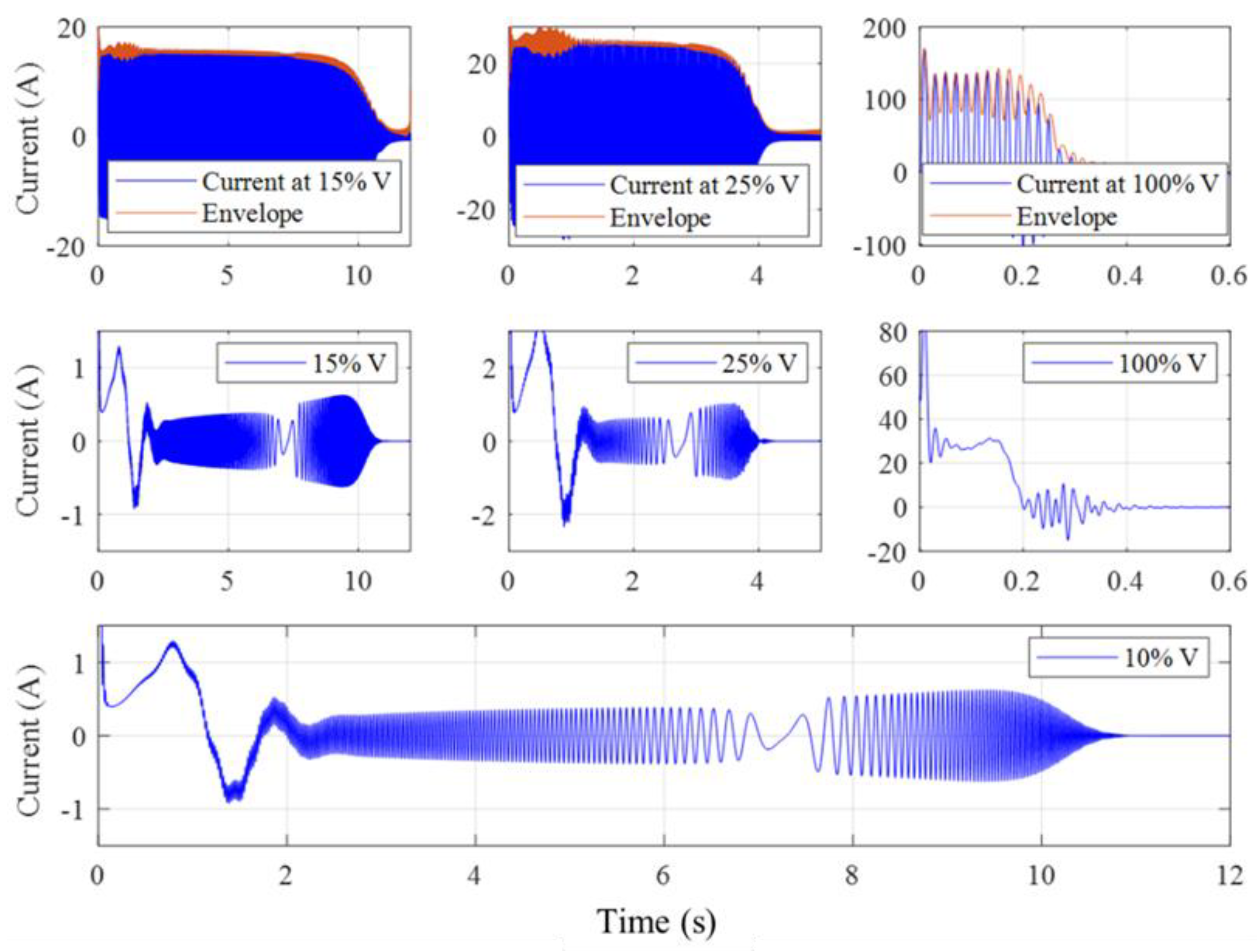
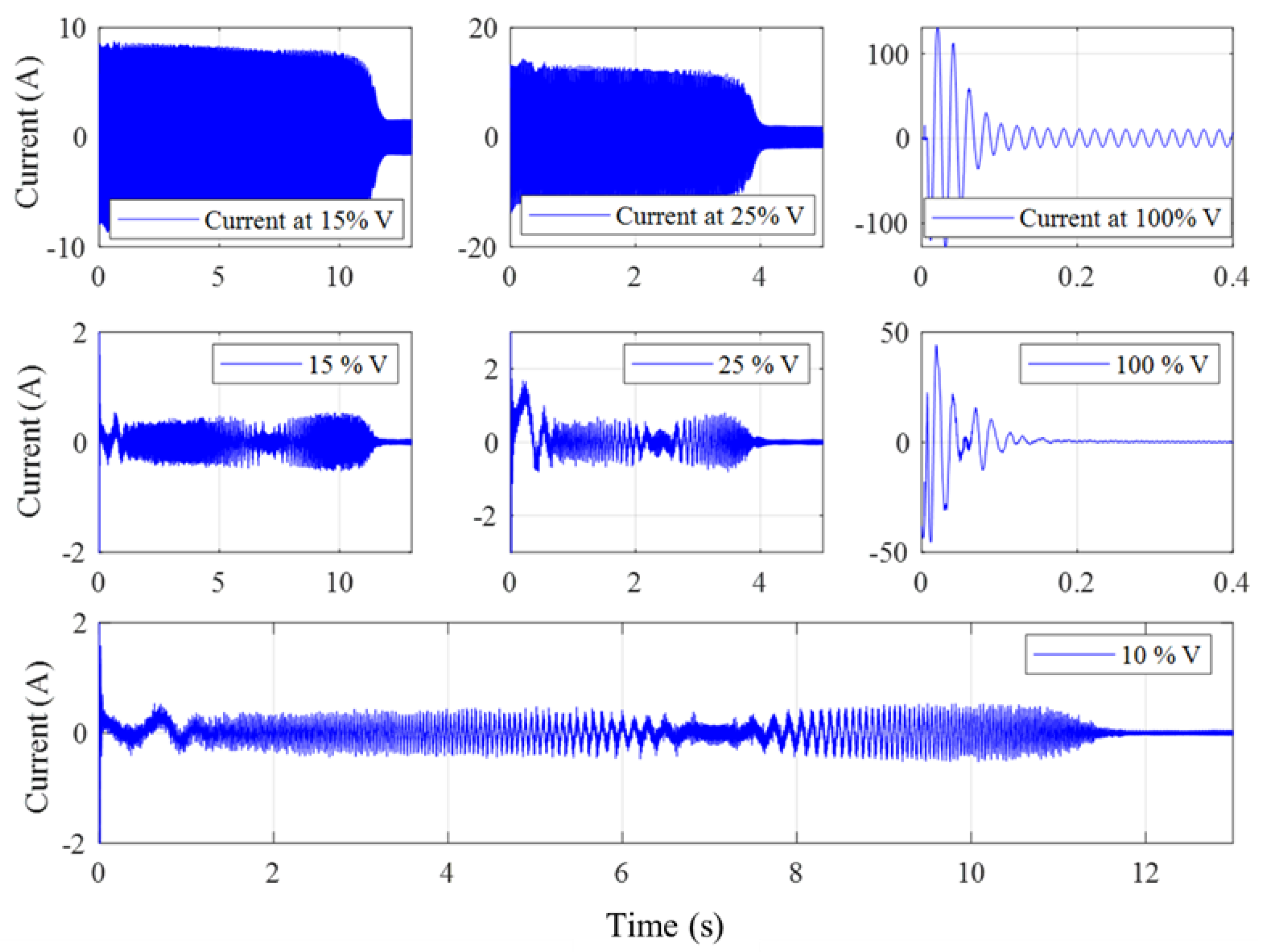
• Unlike most of the papers where a high inertia load or variable transformer is used, an industrial inverter-based low voltage test to extend the motor’s transient interval is proposed. It is also described how an industrial inverter can reduce the voltage while maintaining a constant rated frequency. Increasing the transient length of the motor startup current improves the time–frequency resolution of the spectrum;
• An algorithm to improve the spectrum’s legibility is proposed, which helps segregate various frequency patterns in the transient regime;
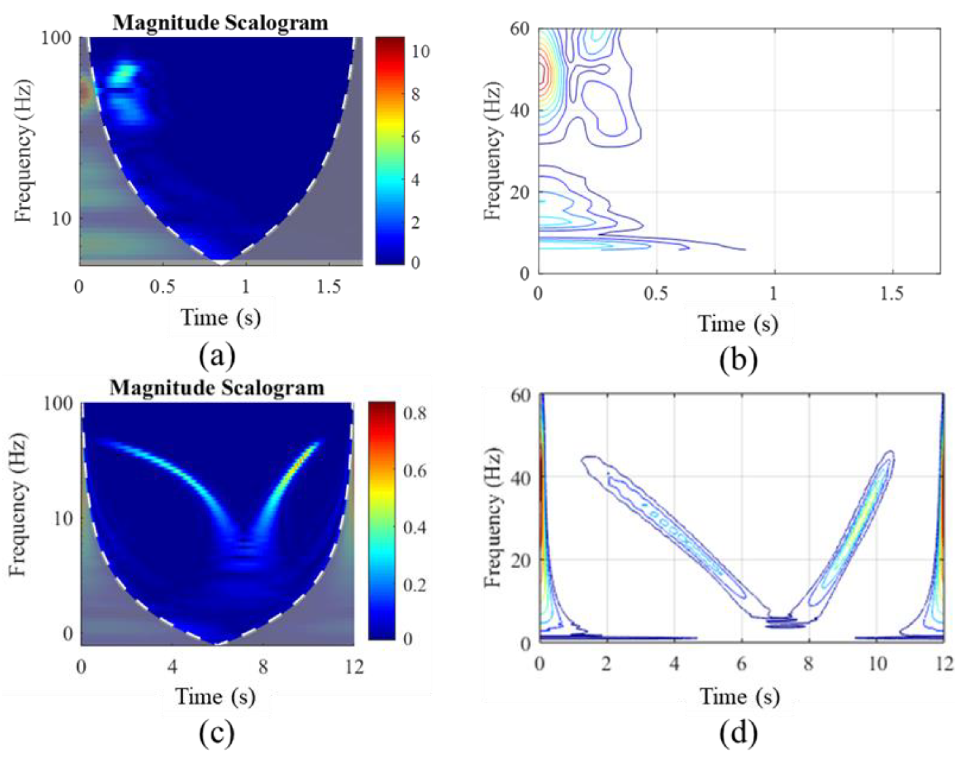
• The wavelet transform is preferred over the short-time Fourier transform (STFT) to avoid inherited FFT drawbacks. Moreover, a band-stop infinite impulse response (IIR) filter is used to attenuate the fundamental component, which improves the spectrum’s legibility;
• It is proposed that the selection of time–frequency regions with a 95% confidence interval (CI) in the form of a contour plot gives a more unambiguous indication of faulty patterns. By adjusting the level of the CI, the spatial and switching frequency-based patterns can be avoided. To the best of the author’s knowledge, this technique is not presented in the literature so far.

2. Theoretical Background

2.1. The Modeling of Induction Motor

Electrical machines’ modeling is the first milestone in machine design, control, analysis and diagnostics. The famous modeling techniques are divided into two major categories: analytic and numerical. The commonly used analytic methods are two-axis theory [25], winding function method (WFM) [26,27,28], reluctance network [29] and convolution theorem-based models [30]. The finite element method (FEM)-based models are typical examples of numerical modeling of electrical machines. Although the numerical models have the least number of approximations, the complexity and computational time is the biggest drawback [31]. It becomes worst in the field of fault diagnostics, where the motor’s symmetry cannot be exploited to reduce the simulation time. For the fault diagnostic in the transient regime, the V-shaped pattern made by the sideband frequencies is significant. This pattern generates because of the varying slip until the steady state region. This nonstationary signal moves in a bandwidth from 0 Hz to 50 Hz. Thus, the higher-order slotting harmonics become less significant for the analysis of the fault-based, nonstationary signal. The winding function-based model with much less complexity than the corresponding FEM-based models is essential to differentiate among several harmonics. Hence, the air gap is considered constant by neglecting the slot openings with the magnetic material’s infinite permeability. The stator winding is approximated as a pure sinusoid, while the rotor turn function represents its actual cage structure. Various self and mutual inductances can be calculated using the winding function formula as in Equation (1). The analytical formulas for the calculation of different inductances given in Equations (2)–(6) are the solution of (1) for the winding functions, as described in [32]:

$$L_{ij}\left(\theta \right)= {\mu }_{o}rl {{\displaystyle \int }}_0^{p\pi }{g}^{-1}\left(\phi ,\theta \right)N_i\left(\phi ,\theta \right)N_j\left(\phi ,\theta \right)d\theta$$

(1)

$$L_m=\frac{{\mu }_{o}rl}{g} \left( \frac{p}{2}\right){\left( \frac{N_s}{p}\right)}^2\pi$$

(2)

$$L_{AB}=L_{BC}=L_{CA}=-\frac{L_m}{2}$$

(3)

$$L_{rkk}=\left(\frac{{\mu }_{o}rl}{g}\right){\mathsf{\alpha }}_r \left[1-\frac{{\mathsf{\alpha }}_r}{p\pi }\right]\left(\frac{p}{2}\right)$$

(4)

$$L_{rki}=\left(\frac{{\mu }_{o}rl}{g}\right)\left[-\frac{{{\mathsf{\alpha }}_r}^2}{p\pi }\right]\left(\frac{p}{2}\right)$$

(5)

$$L_{sri}\left({\theta }_r\right)=\left(\frac{{\mu }_{o}rl{N}_s}{g}\right) \sin (\frac{{\mathsf{\alpha }}_r}{2}) cos({\theta }_r+\left(i-1\right){\mathsf{\alpha }}_r+\frac{{\mathsf{\alpha }}_r}{2})$$

(6)

where μ_o is the permeability of the free space; r is the machine’s radius, which is taken as the center of the air gap; l is the machine’s effective length; g is the air gap width; α_r is the angular displacement between two consecutive rotor bars; p is the number of the poles; Ns is the number of effective turns per phase in the stator; and θ and φ are the rotor and stator angular positions from a reference point. In Equation (6), the inductance is multiplied with a cosine function of θr to emulate the rotating rotor, where integer i changes the angle of the respective rotor bar from the stator reference point. Lm is the magnetization inductance, L_AB, L_BC and L_CA are stator mutual inductances, L_rkk and L_rki are rotor self and mutual inductances and L_sri is the mutual inductance between the stator and rotor.

The performance parameters, such as torque, speed, currents and voltages, can be calculated using Equations (7)–(9):

$$\left[\begin{array}{c}\mathit{V}s\\ 0\end{array}\right]= \left[\begin{array}{cc}{\mathit{R}}_s& 0\\ 0& {\mathit{R}}_r\end{array}\right]\left[\begin{array}{c}{\mathit{I}}_s\\ {\mathit{I}}_r\end{array}\right]+\frac{d}{dt}\left[\begin{array}{cc}{\mathit{L}}_{ss}& {\mathit{L}}_{sr}\\ {\mathit{L}}_{rs}& {\mathit{L}}_{rr}\end{array}\right]$$

(7)

$$T_e= I_s^T(\frac{d}{d\theta }{L}_{rs})I_r$$

(8)

$$J\frac{d}{dt}{\omega }_m= T_e-T_L-B_f{\omega }_m$$

(9)

where Vs is the stator input voltage vector and Rs and Rr are the stator and rotor resistance matrices of orders (3 × 3) and (40 × 40), respectively. Similarly, Lss, Lsr, Lrs and Lss are the matrices containing stator–stator, stator–rotor, rotor–stator, and rotor–rotor self and mutual inductances at a specific rotor position. Moreover, T_e is the generated torque, I_s is the stator current, I_r is the rotor current, T_L is the loading torque, B_f is friction coefficient, ω_m is rotor angular velocity and J is the moment of inertia. The detailed model with slot openings and the actual winding functions can be found in [33].

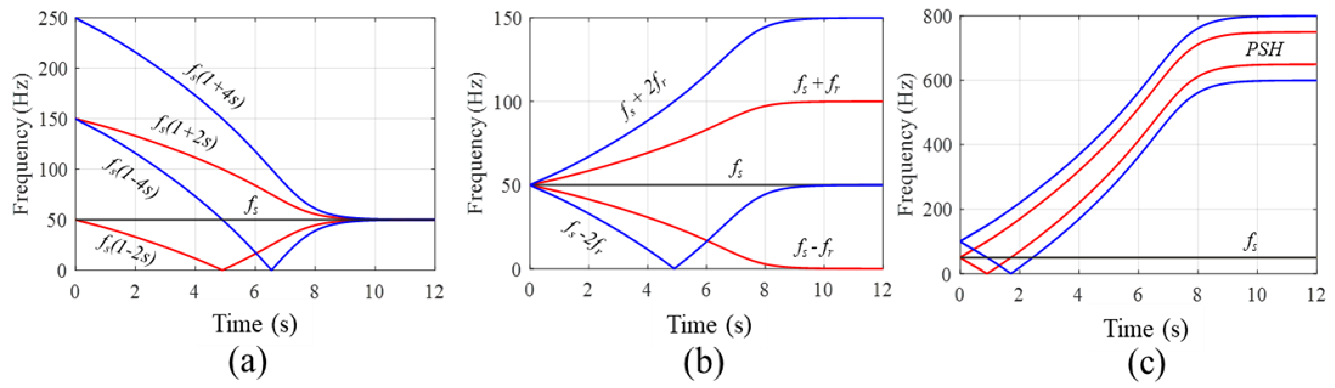
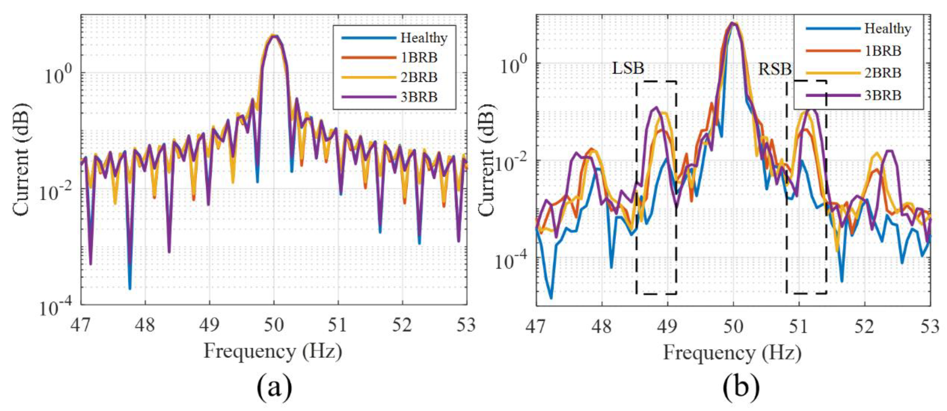
2.2. The Fault Signature Equations and Modulation

Almost all rotor-related faults produce frequency components in the induction motor’s current and the voltage spectrum as a slip function. The most common rotor faults can be diagnosed by detecting the frequencies represented by the equations shown in

Table 1. Fault definition frequencies.

Fault	Modulating Frequencies
Broken Rotor Bars	$f_{BR}=f_s \pm 2ks{f}_s,\hspace{1em}\hspace{1em}k=1, 2, 3,\dots$
PSH and Eccentricity	$f_{ecce}=\left[\left(k{n}_b\pm n_d\right)\left(\frac{1-s}{p}\right) \pm v \right]fs$ More precisely: $f_{ecce}=\left[1\pm k\left(\frac{1-s}{p}\right) \right]fs$ $f_{ecce}= f_s \pm k{f}_r,\hspace{1em}\hspace{1em}k=1, 2, 3,\dots$

where k is the harmonic order, ν is the supply fed harmonics, f_s is the supply frequency, f_br are the broken bar frequencies, n_d is the dynamic eccentricity (0 for static and 1, 2, 3…. for dynamic), f_r is rotor frequency, s is the slip and p is the number of poles.

.

The phase current of an ideal and symmetrical machine can be defined as

$$i_a\left(t\right)=I_m sin\left(\omega t+\alpha \right)$$

(10)

where Im is the peak current, ω is the supply frequency in the angular domain and α is the phase angle. The unsymmetrical rotor with broken rotor bars, broken end rings or bad bearings starts modulating the current with a frequency dependent upon the rotor’s speed and the modulation index, which depends upon the severity of the fault:

$$i_{af}\left(t\right)=\left[1+m\left(t\right)\right]i_a\left(t\right)$$

(11)

where m(t) is the modulating signal having a modulation index M, which depends on the number of broken bars (Nb) and the total number of rotor bars (Nt). If the rotor is rotating and the winding distributions are considered as sinusoidal, the modulating signal is also a sinusoid, such that

$$m\left(t\right)=Mcos\left({\omega }_{o}t+ \phi \right)$$

(12)

where ω_o = 2πf is the fault characteristic frequency and depends on its nature and the machine’s slip. In the case of the broken rotor bars, the characteristic fault frequency is at 2sf_s:

$$i_{af}\left(t\right)=\left[1+Mcos\left(4\pi s{f}_{s}t+ \phi \right)\right]i_a\left(t\right)$$

(13)

$$f_o=2s{f}_s and {\omega }_o=2\pi \left(2s{f}_s\right)$$

(14)

$$m\left(t\right)=Mcos\left(4\pi s{f}_{s}t+ \phi \right)$$

(15)

$$i_{af}\left(t\right)=\left[1+Mcos\left(4\pi s{f}_{s}t+ \phi \right)\right]I_m sin\left(\omega t\right)$$

(16)

$$i_{af}\left(t\right)=I_m sin\left(2\pi f_{s}t\right)+\left(\frac{M{I}_m}{2}\right)\left[sin\left(2\pi f_s\left(1+2s\right)t+\phi \right)+ sin\left(2\pi f_s\left(1-2s\right)t+\phi \right)\right]$$

(17)

The modulation index M can be approximated as a ratio between the number of broken and total rotor bars [34]:

$$M \approx \raisebox{1ex}{$N_b$}\!\left/ \!\raisebox{-1ex}{$N_t$}\right.$$

(18)

The sine terms with frequencies fs(1 + 2s) and fs(1 − 2s) in Equation (17) correspond to the right-hand side (RHS) and left-hand side (LHS) harmonics, which makes a pattern during the transient regime as the slip changes from the maximum value to some specific value, depending upon the load.

In the steady state current, each fault is represented with a particular frequency value, as described previously. In the transient region, the frequency changes continuously. The rapidly evolving slip in the transient regime gives rise to nonstationary signals making specific patterns. The most common causes are the rotor asymmetries, such as the inherent eccentricity, the principal slotting harmonics and the broken bars or end rings. Figure 1 presents the theoretical development of those patterns for a harmonic order of two.

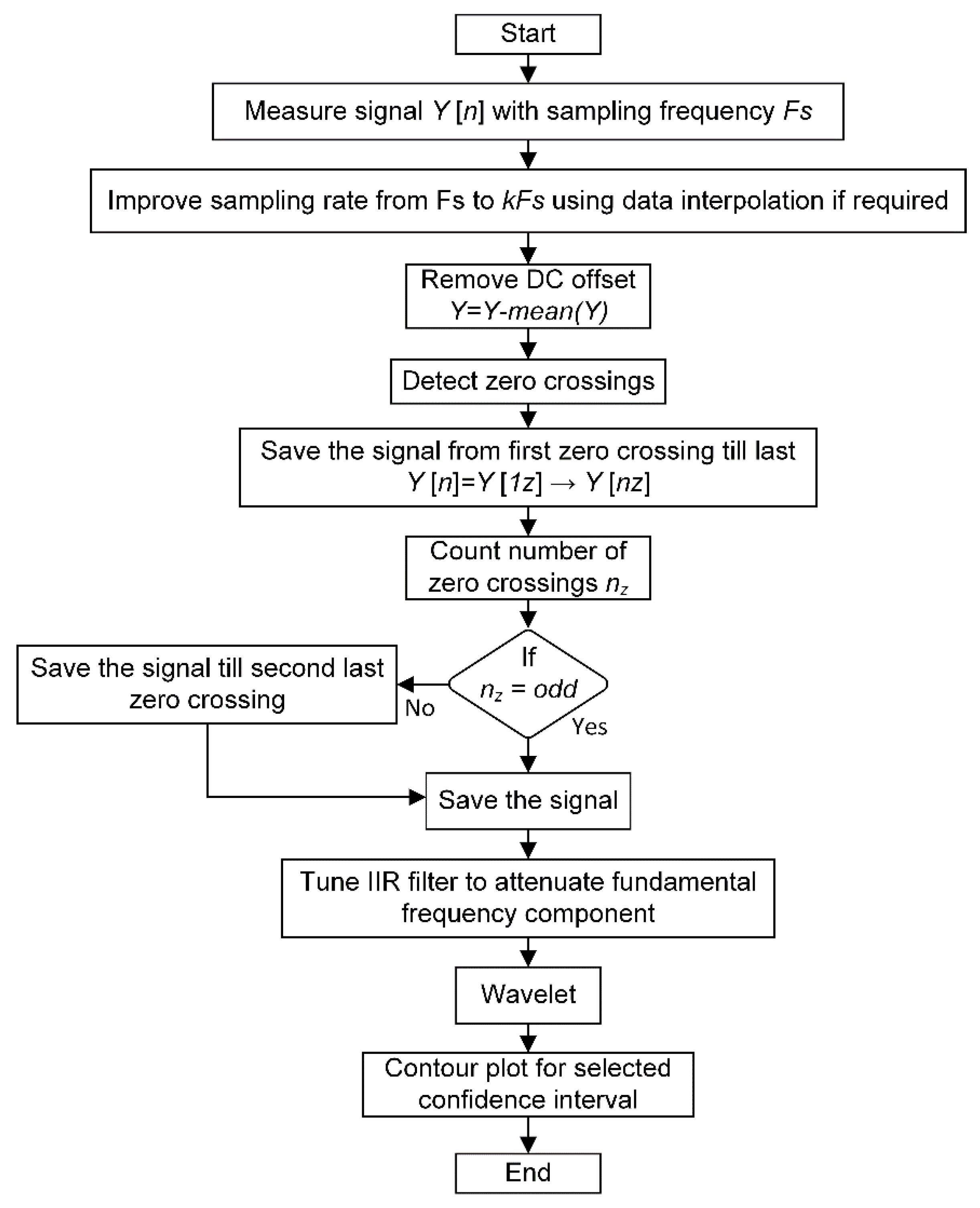
2.3. The Recovery of the Nonstationary Signal and Related Signal Processing

The frequency spectrum’s legibility in either a steady state or transient regime depends on the signal’s length and sampling frequency. The fault-representing frequencies are the function of motor slip, as described in Table 1. During the transient interval, the slip is not constant, but decreases with an increase in speed as the motor goes toward a steady state regime. This changing slip results in the creation of nonstationary signals in the transient domain. With a rated supply, this transient interval is so small that those patterns do not become visible. It becomes worse when the motor operates at a low load. The transient interval can be extended by decreasing the supply voltage with a high inertia load, while the input voltage can be changed using a variable three-phase transformer or an industrial inverter. The increasing use of the frequency converter as a substantial part of the drive system increases the test’s feasibility. By reducing the supply voltage while maintaining a constant frequency, the rotor’s inertia can control the transient time of the motor. Moreover, with reduced voltage, the leakage inductance also takes more time to reach the steady state point, which also supports an extended transient interval. For any reliable signal processing-based diagnostic algorithm, the role of digital filters is undeniable.

Digital filters are the mathematical algorithms capable of reducing or enhancing specific parameters of a signal. They are used for either the separation of combined signals or the restoration of a distorted signal. Their diversified nature has many types, and they are being used extensively in almost every signal processing-based application.

They are the potential tool to remove the strong supply-based frequency components for improving the time–frequency spectrum’s legibility. This is necessary because the fundamental component is powerful in amplitude compared with the fault-based harmonics, which are very weak, particularly at the fault’s embryonic stage. Those low-amplitude frequency components become barely visible in the presence of the fundamental component.

To attenuate the fundamental component, the selection of an appropriate band-stop filter becomes very crucial. The infinite impulse response (IIR) band-stop filters, such as the Chebyshev II, can give promising results because of their steep transition band and low passband ripples among various digital filters. The excellent transition band and low passband ripples can reduce the filter’s impact on the recovered signal.

In light of the mentioned theoretical aspects, the frequency spectrum resolution for transient and steady signals is improved in the following way, as presented in Figure 2:

• Measure the signal with the sampling frequency, meeting the Nyquist criterion. The sampling frequency can be improved later using data interpolation. This is necessary for the accurate detection of zero-crossing points. Moreover, any small constant offset due to data acquisition devices should be removed to avoid a high-amplitude 0 Hz component in the spectrum. This is achieved by subtracting the mean value of the signal from itself;
• Most signal processing techniques, such as DTFT, are sensitive to signal discontinuities and the fractional number of acquired cycles. This problem is solved by counting the integral number of cycles using zero-crossing detection. Saving the signal from the first until the last zero crossings will remove the starting and ending fractional portions of the signal;
• Each sinusoidal signal has three zero crossings, which can be exploited to get the integral number of cycles. If the number of zero crossings is odd, then the signal consists of an integral number of cycles; otherwise, the samples from the second-last zero-crossing until the end should be discarded;
• The band-stop IIR filter is then tuned to suppress the fundamental component;
• The recovered signal shows good spectral legibility both for frequency (steady state) and time–frequency (transient) analysis.

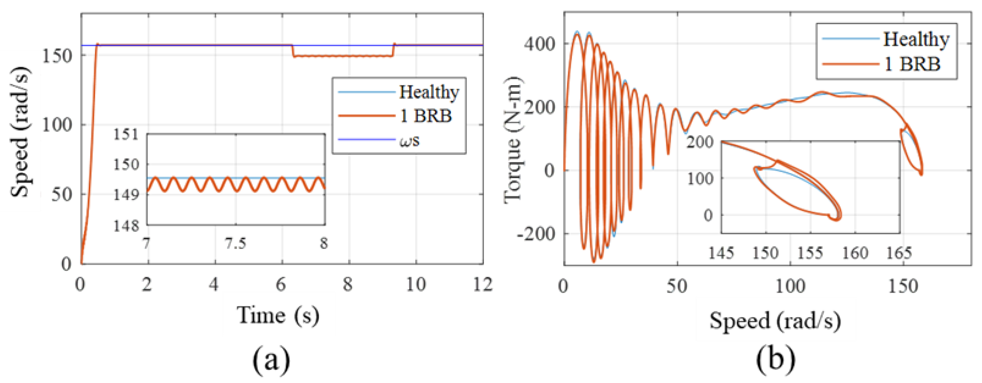
3. Simulation Results

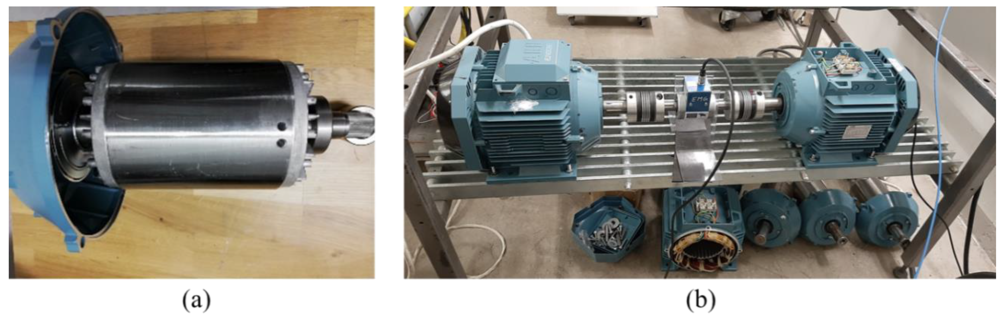
The winding function model described in Section 2 was used for the transient and steady-state analysis of the motor’s performance parameters under healthy and broken bar conditions. The broken bars were simulated by increasing the value of corresponding entries in the resistance matrix. Figure 3b shows the speed–torque dynamic response under healthy and faulty conditions. The zoomed window shows the shift of the operating point at the load application with a slight increase in the slip. The speed and torque ripples due to broken bars are visible in Figure 3a,b.

These ripples were because of the fault-based induced voltage on the stator side. The frequency of those harmonics depended upon the slip, as discussed previously. During the transient interval, the slip changed dramatically from one to the nominal value, generating a nonstationary signal in the current. This transient interval was so narrow that any specific pattern was hardly visible with rated voltage conditions because of the low-frequency resolution. This phenomenon is described in Figure 4. The motor’s simulated transient current at 10%, 15%, 25%, and the rated voltage is presented. The envelope is highlighted by plotting the absolute value of the analytical function given below in (19) and (20). In all subfigures, the x-axis represents the time in seconds while the y-axis represents the amplitude in amperes. Moreover, as the constant air-gap is considered in the simulation model, the non-stationary signal contains only broken bar based pattern.

$$i_A\left(t\right)=i\left(t\right)+j \widehat{i}\left(t\right)$$

(19)

where i(t) is the current, j is the imaginary unit representing the complex number and i^{^}(t) is its Hilbert-transformed signal. This can be achieved by the convolution of the signal with 1/πt, as shown by the following equation:

$$H\left(t\right)=\frac{1}{\pi }{{\displaystyle \int }}_{-\infty }^{\infty }\left(\frac{f\left(x\right)}{t-x}\right)dx$$

(20)

All these steps can be achieved in Matlab by using the simple command ab (hilbert(i[t])). The envelope contains all harmonics other than the fundamental component. For a steady state signal, the Hilbert filter is the right choice for attenuation of the fundamental component. However, in the transient regime, the phase shift of all frequency components poses a problem.

Hence, the nonstationary current signatures were recovered by attenuating the fundamental component using the IIR band-stop filter, as shown in Figure 4 (middle and last row). With a decrease in the applied voltage, the fault-based nonstationary signal increased in length and became more legible. The time–frequency analysis of those non-stationary signals at rated voltage and 10% of the rated voltage is shown in Figure 5. With reduced voltage and the corresponding increase in the signal length, the V-shaped pattern became visible, being hardly present in the current at the rated voltage. Moreover, the supply frequency component (50 Hz) was attenuated using the proposed filter. The fault pattern became more legible by using filter and contour plots together. The contour plot shows the areas with a 95% confidence interval. With the rated voltage, the total power was confined in the region until 0.5 s without any pattern (Figure 5b), while with extended time, the pattern became visible as in Figure 5d. In the magnitude scalogram, the color bar represents the amplitude of the specific frequency component in amperes.

4. Practical Setup

The test rig consisted of a motor under investigation attached with a loading machine, industrial inverters and a data acquisition set-up. The motor, with specifications given in

Table 2. The machine specifications.

Parameter	Symbol	Value
Number of poles	P	4
Number of phases	φ	3
Connection	-	Delta
Stator slots	Ns	36, non-skewed
Rotor bars	Nb	28, skewed
Rated voltage	V	400 V@50 Hz
Rated current	I	8.8 A
Rated power	Pr	7.5 kW @ 50 Hz

, was tested with healthy and broken bar-based rotors. The bars were broken by drilling radial holes having a depth equal to the total rotor slot height. The motor phase currents were measured under transient intervals using the Dewetron transient recorder. The measured signal’s sampling frequency was 10 kHz, which was good enough for better frequency resolution. The test set-up is shown in Figure 6. In the industrial inverter case, the variable voltage at a constant frequency could be achieved by changing the rated parameters. Since the voltage/Hz ratio in the scalar control remained constant, by changing the rated frequency with a constant rated voltage, the output voltage could be varied, as shown in

Table 3. The setting of the industrial inverter to achieve the desired voltage.

Vrated (V)	frated (Hz)	V/Hz	fset (Hz)	Vout (V)
300	300	1	50	50
300	150	2	50	100
300	100	3	50	150
300	75	4	50	200
300	60	5	50	250
300	50	6	50	300

. Moreover, the acceleration and deceleration time should be equal to zero to avoid the drive controller’s influence on the transient interval.

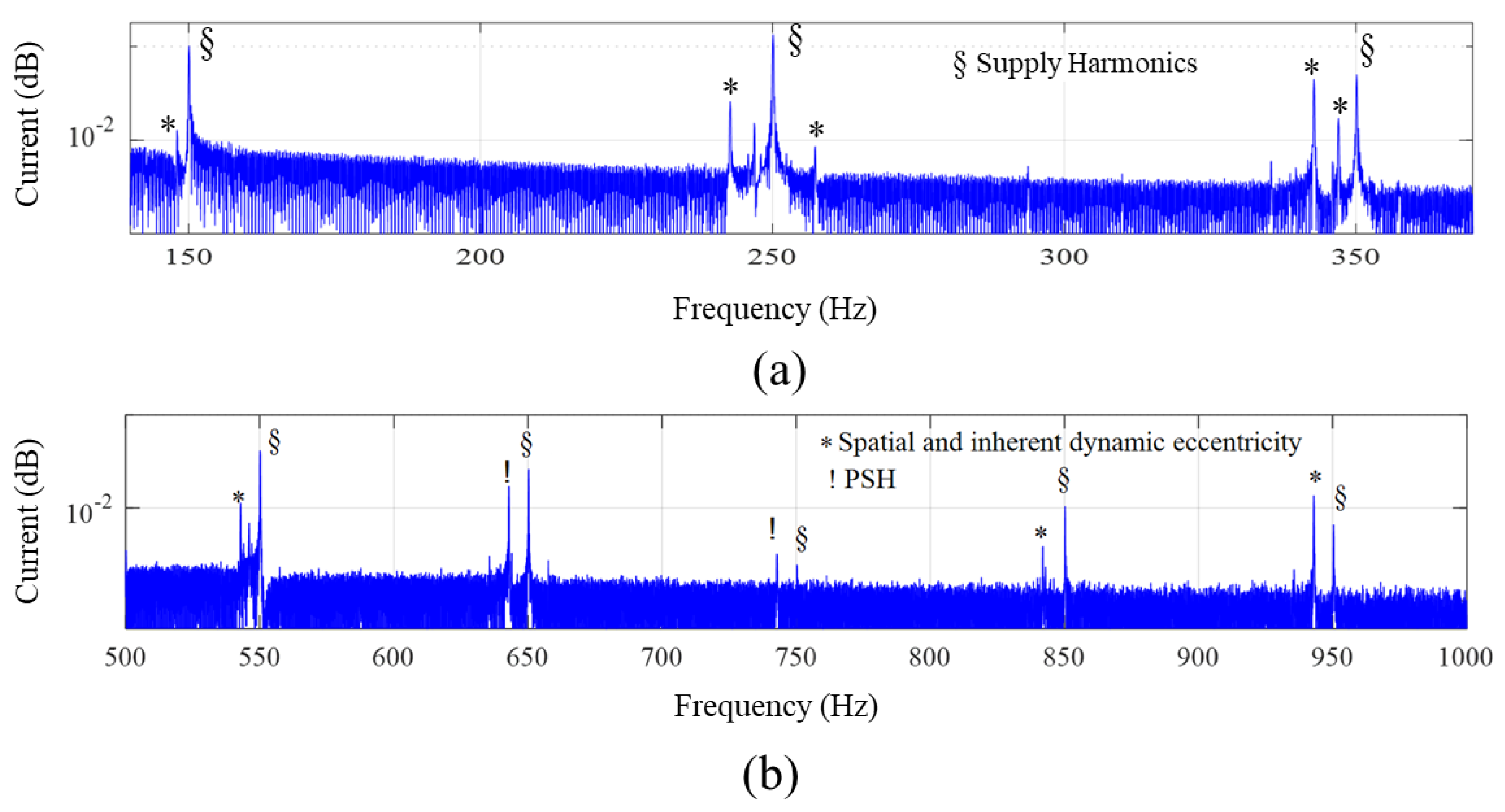
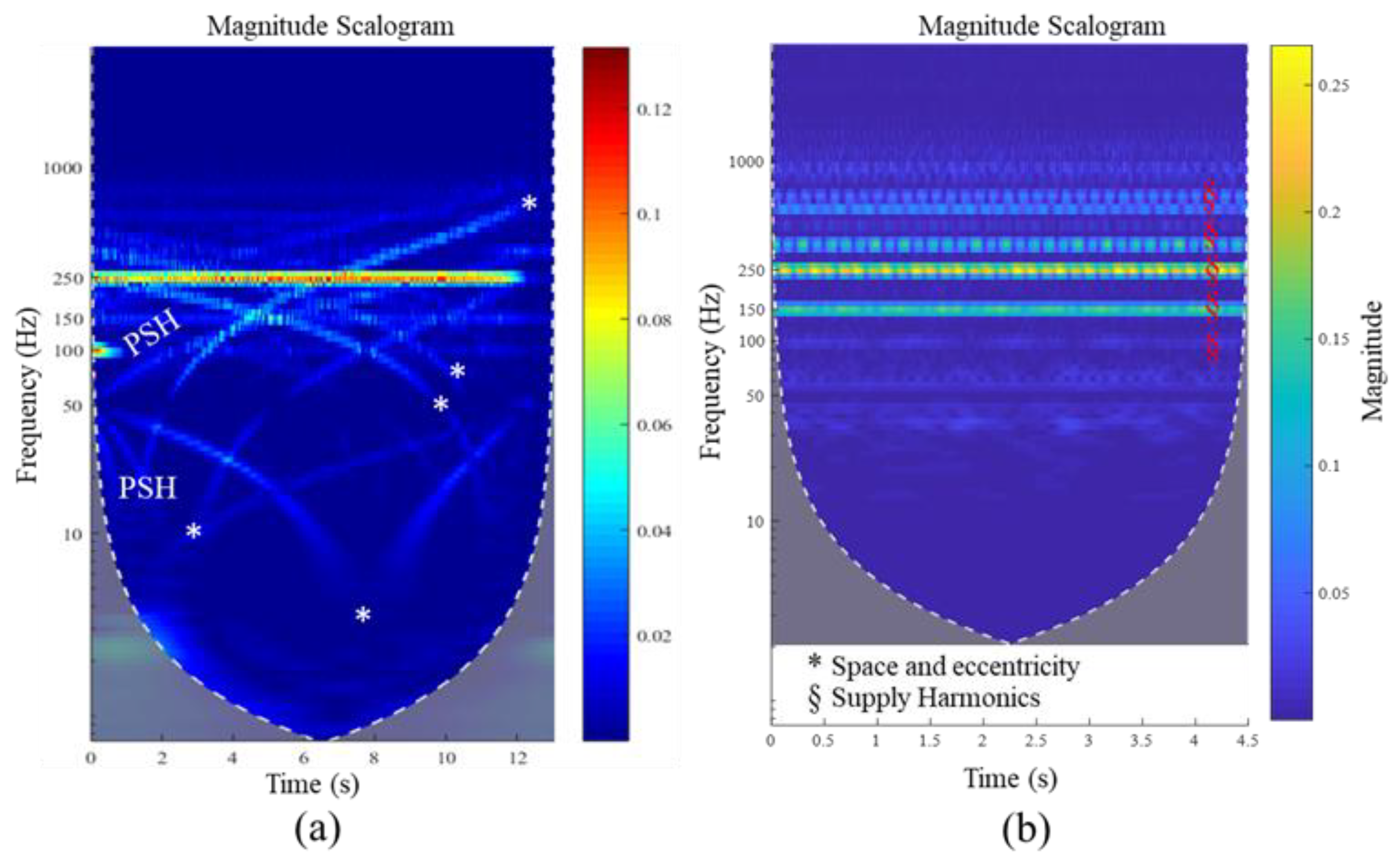
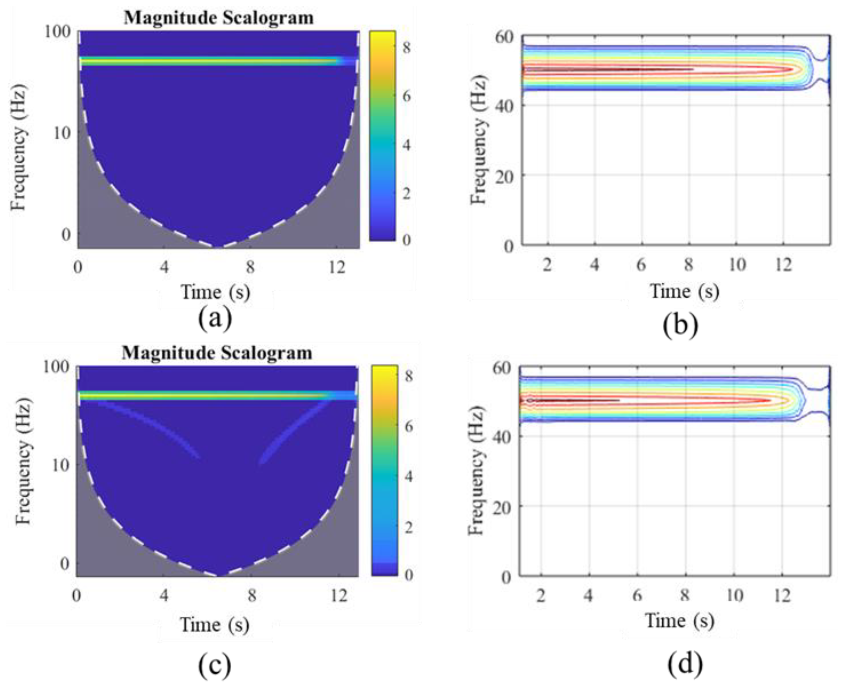
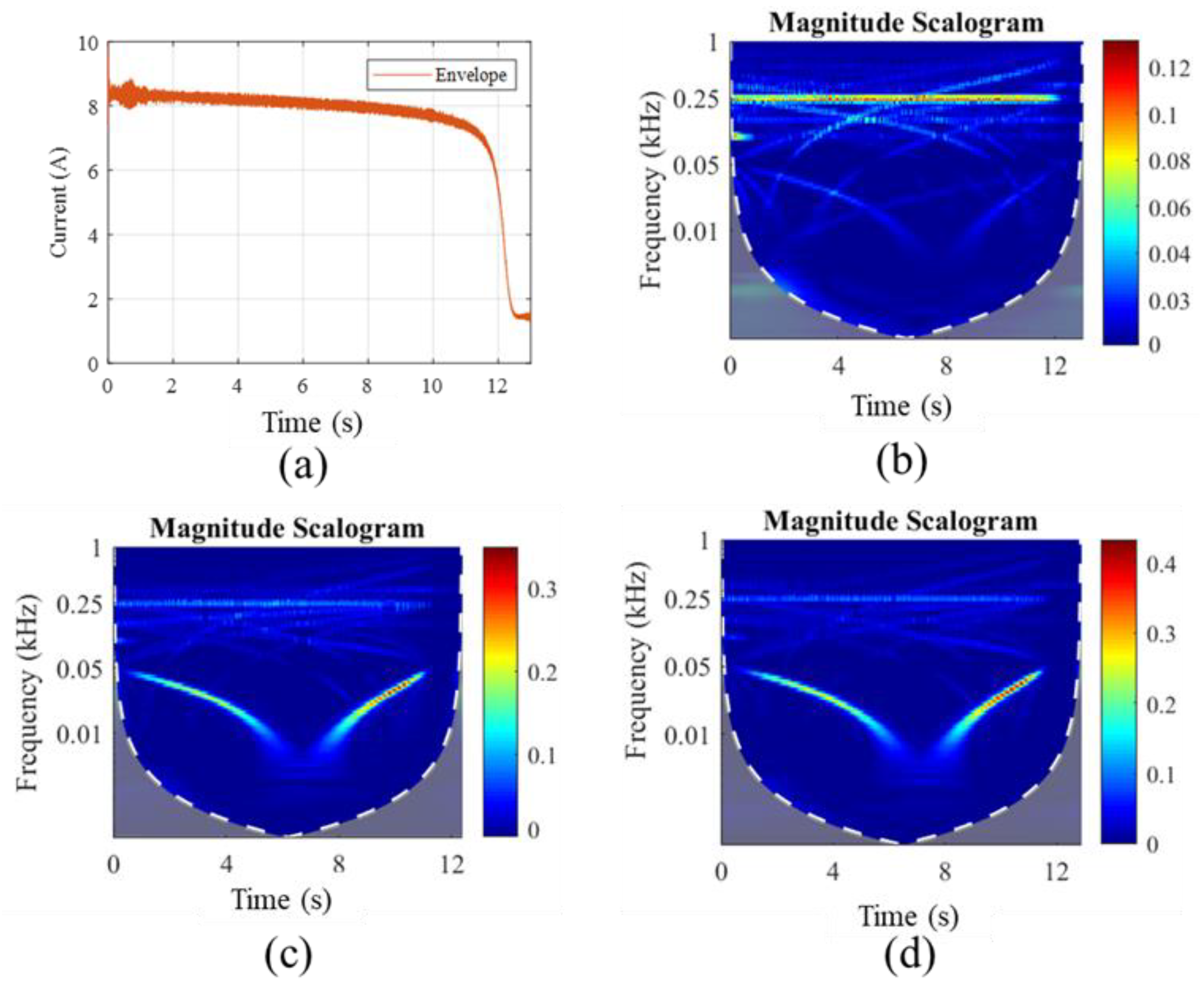
5. Results and Discussion

Figure 7 shows the motor’s transient current at 15%, 25% and 100% of the rated supply voltage with two broken bars. The recovered nonstationary signal was very legible at 10% of the supply voltage. Unlike the simulation-based results, these signals contained several higher-order harmonics. The most prominent causes of those harmonics were the non-sinusoidal stator and rotor winding distribution, the stator, the rotor slot openings and the magnetic material’s nonlinear behavior. However, those frequency components were of less significance, as the most prominent fault-based pattern remained in the bandwidth of 0–50 Hz.

The frequency spectrum of the stator current during the steady state interval for healthy and broken rotor bars at no load and rated load conditions is shown in Figure 8. The spectrum in Figure 8b shows the evolution of the left-side band (LSB) and right-side band (RSB) harmonics. These harmonics are the function of slip, and the results are based on the measurements taken under rated load conditions.

The sideband frequencies increased in amplitude with the increase in the number of broken bars. Besides that, the sideband fault frequencies tended to shift slightly away from the fundamental component with the rise in broken bars. With the increase in the number of broken bars, the average generated torque decreased with a slight rise in slip. The segregation of these components is very difficult from the rest of the harmonics if the entire spectrum is considered.

The severity of this problem increases with the decrease in load. As the load decreased, these harmonics started hiding under the fundamental component, with total disappearance at the no load condition as in Figure 8a. Moreover, the skewness in the rotor and stator slots affected their amplitudes, making them less detectable at the developing stage. The skews tended to attenuate the rotor harmonics for smooth speed torque features. It is also important to mention that these harmonics remain venerable when the inverter feeds the motor. This effect can be in the form of a colossal number of harmonics fed by the inverter, making faulty frequencies even more difficult for segregation. Moreover, the impact of the drive controller cannot be ignored. This impact is worst in DTC-controlled motors, where the controller of the drive tries to eliminate the current harmonics to reduce torque ripples [14].

The leading causes of the speed and torque ripples were the current harmonics, due to non-sinusoidal winding distribution on the stator and rotor side, the supply-based odd multiples of the fundamental component even if the machine was grid-fed, the inherent dynamic eccentricity and the magnetic material’s nonlinear behavior. Those harmonics are inevitable, even if the machine is in a healthy condition. Figure 9 shows those harmonics in the stator current spectrum of a grid-fed healthy motor working under 50% of the rated load. All the harmonics except the supply-fed one were the function of slip and tended to move away from the parent supply component with the increase in load. As discussed earlier, the legibility of those harmonics in the current spectrum not only depended upon slip but the fluctuating load, and the drive’s controller also made the detection of desired components challenging.

To avoid all those problems, the inspection of the motor current under the transient regime showed promising results. For an increase in the transient time for better time–frequency resolution, the supply voltage could be reduced using a three-phase transformer or the industrial inverter, as discussed previously. With the increase in the applied voltage, the motor took less time to reach a steady state interval. Under the transient regime, the continuously decreasing slip moved the RHS and LHS frequency components toward the fundamental component. It made a V-shaped pattern whose width depended upon the transient time. An exceptional intention was needed here, as there were several slip-dependent frequency components, which could make similar patterns in the transient region. Those frequencies are the spatial and inherent dynamic eccentricity-based harmonics, which develop near all supply-fed higher-order harmonics.

Figure 10 shows the harmonics’ development in the transient and steady state regime under the healthy condition with the attenuated fundamental component. It is evident that in the transient region, the rotor slotting and eccentricity-based harmonics made the V-shaped patterns, as in Figure 10a. Those patterns started from 50 Hz and vanished completely as they approached the parent supply component, as in Figure 10b. It is essential to differentiate them from the actual faulty patterns to avoid false alarms.

Figure 11 shows the time–frequency response, with the respective regions containing 85% of the total spectral energy in the contour plot for the healthy and broken bar cases. In the presence of the fundamental component, the faulty pattern is barely visible even in the extended current, as in Figure 11c. Moreover, the influence of the most potent supply component on the visibility of the fault pattern is evident in the contour plot. Although the faulty pattern is visible to some extent in the magnitude scalogram, it is absent in the contour plot, as the maximum spectral energy remained in the region near the fundamental component.

This pattern was not very legible because the sideband frequencies were lower in amplitude than the fundamental component. This pattern can be made very clear by attenuating the fundamental component, as shown in Figure 12. The IIR band-stop filter, having a filter order of two and a stopband attenuation of 40 showed promising results, while attenuating a narrow bandwidth of frequencies from 49.9 Hz to 50.1 Hz. Figure 12a shows the transient current envelope, while the evolution of spatial frequencies in the transient regime is presented in Figure 12b. The development of a faulty pattern with good legibility is shown in Figure 12c,d for one and two broken bars, respectively.

The contour plot with a bump mother wavelet for the healthy and one broken rotor bar (BRB) cases is shown in Figure 13. Since the spatial harmonics were weaker than the fault frequencies, the contour plot shows the evolution of the sideband frequencies, which avoids confusion with the slotting-related patterns.

6. Conclusions

The broken rotor bars fault diagnostics by time–frequency analysis of the motor current under the transient period was investigated in this paper. The detection of fault frequencies in the steady state interval was prevalent in the literature but possessed several difficulties. Since the sideband frequencies were the function of slip, they became challenging to discover under low-load conditions. The spectral leakage of the prevailing supply components was hazardous for the visibility of faulty components, as they were fragile in amplitude. The spectral leakage was the function of the signal length, the sampling frequency and the type of window used to compute the FFT or wavelet.

Moreover, the inclusion of a vast bandwidth of inverter-fed frequencies made the detection of faulty frequencies hazier. The drive controller’s impact on reducing the current ripples was another fact, making fault diagnosis under a steady state regime difficult.

These drawbacks can be resolved by investigating the health in the transient regime. The transient interval’s biggest flaw is the little time, which reduces the resolution of the spectrum. This transient time can be increased by lowering the applied voltage without any external load. By doing so, the broken bars-based V-shaped pattern can be seen with great accuracy. Moreover, the FFT-based drawbacks are considerably reduced by using the wavelet approach. The transient spectrum’s legibility is further enhanced by attenuating the fundamental component with an IIR filter’s help. The IIR band-stop filter has a sharp transition interval and low passband ripples, having less influence on the remaining frequency components.

Several spatial and supply-related frequency patterns can cause a false alarm if they are not differentiated accurately from the actual faulty components. Those components are much weaker in amplitude compared with the fault-related frequencies. The use of the filter to attenuate those components is nearly impossible, as they are not stationary. Hence, the regions with the maximum spectral energy in the form of a contour plot are used, which can be easily adjusted as a threshold to show the pattern. The results are presented using the simulations and the measurements taken from a laboratory-based test rig.

The proposed approach can be used for the pattern-based training of advanced artificially intelligent (AI) diagnostic algorithms.

References

1. Bossio, G.R.; De Angelo, C.H.; Bossio, J.M.; Pezzani, C.M.; Garcia, G.O. Separating Broken Rotor Bars and Load Oscillations on IM Fault Diagnosis Through the Instantaneous Active and Reactive Currents. IEEE Trans. Ind. Electron. 2009, 56, 4571–4580. [Google Scholar] [CrossRef]
2. Soualhi, A.; Clerc, G.; Razik, H. Detection and Diagnosis of Faults in Induction Motor Using an Improved Artificial Ant Clustering Technique. IEEE Trans. Ind. Electron. 2013, 60, 4053–4062. [Google Scholar] [CrossRef]
3. Marques Cardoso, A.J.; Saraiva, E.S. On-line diagnostics of three-phase induction motors by Park’s vector. In Proceedings of the ICEM, Pisa, Italy, 12–14 September 1988; pp. 231–234. [Google Scholar]
4. Oliveira, L.M.R.; Cardoso, A.J.M. Extended Park’s vector approach-based differential protection of three-phase power transformers. IET Electr. Power Appl. 2012, 6, 463. [Google Scholar] [CrossRef]
5. Freire, N.M.A.; Estima, J.O.; Marques Cardoso, A.J. Open-Circuit Fault Diagnosis in PMSG Drives for Wind Turbine Applications. IEEE Trans. Ind. Electron. 2013, 60, 3957–3967. [Google Scholar] [CrossRef]
6. Cruz, S.M.A.; Cardoso, A.J.M. Stator winding fault diagnosis in three-phase synchronous and asynchronous motors, by the extended Park’s vector approach. IEEE Trans. Ind. Appl. 2001, 37, 1227–1233. [Google Scholar] [CrossRef]
7. Cruz, M.A.; Marques Cardoso, S.A.J. Rotor Cage Fault Diagnosis in Three-Phase Induction Motors by Extended Park’s Vector Approach. Electr. Mach. Power Syst. 2000, 28, 289–299. [Google Scholar]
8. Ayhan, B.; Trussell, H.J.; Chow, M.Y.; Song, M.H. On the Use of a Lower Sampling Rate for Broken Rotor Bar Detection With DTFT and AR-Based Spectrum Methods. IEEE Trans. Ind. Electron. 2008, 55, 1421–1434. [Google Scholar] [CrossRef] [Green Version]
9. Khezzar, A.; Kaikaa, M.Y.; El Kamel Oumaamar, M.; Boucherma, M.; Razik, H. On the Use of Slot Harmonics as a Potential Indicator of Rotor Bar Breakage in the Induction Machine. IEEE Trans. Ind. Electron. 2009, 56, 4592–4605. [Google Scholar] [CrossRef]
10. Malekpour, M.; Phung, B.T.; Ambikairajah, E. Stator current envelope extraction for analysis of broken rotor bar in induction motors. In Proceedings of the 2017 IEEE 11th International Symposium on Diagnostics for Electrical Machines, Power Electronics and Drives (SDEMPED), Tinos, Greece, 29 August–1 September 2017; pp. 240–246. [Google Scholar]
11. Belahcen, A.; Martinez, J.; Vaimann, T. Comprehensive computations of the response of faulty cage induction machines. In Proceedings of the 2014 International Conference on Electrical Machines (ICEM), Berlin, Germany, 2–5 September 2014; IEEE: Piscataway, NJ, USA, 2014; pp. 1510–1515. [Google Scholar]
12. Nandi, S.; Toliyat, H.A.; Li, X. Condition Monitoring and Fault Diagnosis of Electrical Motors—A Review. IEEE Trans. Energy Convers. 2005, 20, 719–729. [Google Scholar] [CrossRef]
13. Asad, B.; Vaimann, T.; Kallaste, A.; Belahcen, A. Harmonic Spectrum Analysis of Induction Motor With Broken Rotor Bar Fault. In Proceedings of the 2018 IEEE 59th International Scientific Conference on Power and Electrical Engineering of Riga Technical University (RTUCON), Riga, Latvia, 12–13 November 2018; pp. 1–7. [Google Scholar]
14. Asad, B.; Vaimann, T.; Belahcen, A.; Kallaste, A.; Rassõlkin, A.; Iqbal, M.N. Broken rotor bar fault detection of the grid and inverter-fed induction motor by effective attenuation of the fundamental component. IET Electr. Power Appl. 2019, 13, 2005–2014. [Google Scholar] [CrossRef]
15. Puche-Panadero, R.; Pineda-Sanchez, M.; Riera-Guasp, M.; Roger-Folch, J.; Hurtado-Perez, E.; Perez-Cruz, J. Improved Resolution of the MCSA Method Via Hilbert Transform, Enabling the Diagnosis of Rotor Asymmetries at Very Low Slip. IEEE Trans. Energy Convers. 2009, 24, 52–59. [Google Scholar] [CrossRef]
16. Pineda-Sanchez, M.; Riera-Guasp, M.; Antonino-Daviu, J.A.; Roger-Folch, J.; Perez-Cruz, J.; Puche-Panadero, R. Diagnosis of Induction Motor Faults in the Fractional Fourier Domain. IEEE Trans. Instrum. Meas. 2010, 59, 2065–2075. [Google Scholar] [CrossRef]
17. Moussa, M.A.; Boucherma, M.; Khezzar, A. A Detection Method for Induction Motor Bar Fault Using Sidelobes Leakage Phenomenon of the Sliding Discrete Fourier Transform. IEEE Trans. Power Electron. 2017, 32, 5560–5572. [Google Scholar] [CrossRef]
18. Kia, S.H.; Henao, H.; Capolino, G.-A. Diagnosis of Broken-Bar Fault in Induction Machines Using Discrete Wavelet Transform Without Slip Estimation. IEEE Trans. Ind. Appl. 2009, 45, 1395–1404. [Google Scholar] [CrossRef]
19. Singh, S.; Kumar, N. Detection of Bearing Faults in Mechanical Systems Using Stator Current Monitoring. IEEE Trans. Ind. Inform. 2017, 13, 1341–1349. [Google Scholar] [CrossRef]
20. Kang, M.; Kim, J.-M. Reliable Fault Diagnosis of Multiple Induction Motor Defects Using a 2-D Representation of Shannon Wavelets. IEEE Trans. Magn. 2014, 50, 1–13. [Google Scholar] [CrossRef]
21. Sapena-Bano, A.; Pineda-Sanchez, M.; Puche-Panadero, R.; Martinez-Roman, J.; Matic, D. Fault Diagnosis of Rotating Electrical Machines in Transient Regime Using a Single Stator Current’s FFT. IEEE Trans. Instrum. Meas. 2015, 64, 3137–3146. [Google Scholar] [CrossRef] [Green Version]
22. Antonino-Daviu, J. Electrical monitoring under transient conditions: A new paradigm in electric motors predictive maintenance. Appl. Sci. 2020, 10, 6137. [Google Scholar] [CrossRef]
23. Gyftakis, K.N.; Spyropoulos, D.V.; Mitronikas, E. Advanced Detection of Rotor Electrical Faults in Induction Motors at Start-up. IEEE Trans. Energy Convers. 2020. [Google Scholar] [CrossRef]
24. Gyftakis, K.N.; Panagiotou, P.A.; Lee, S. Bin Generation of Mechanical Frequency Related Harmonics in the Stray Flux Spectra of Induction Motors Suffering from Rotor Electrical Faults. IEEE Trans. Ind. Appl. 2020, 56, 4796–4803. [Google Scholar] [CrossRef]
25. Cunha, C.C.M.; Lyra, R.O.C.; Filho, B. Simulation and Analysis of Induction Machines With Rotor Asymmetries. IEEE Trans. Ind. Appl. 2005, 41, 18–24. [Google Scholar] [CrossRef]
26. Faiz, J.; Ojaghi, M. Unified winding function approach for dynamic simulation of different kinds of eccentricity faults in cage induction machines. IET Electr. Power Appl. 2009, 3, 461. [Google Scholar] [CrossRef]
27. Nandi, S. Modeling of Induction Machines Including Stator and Rotor Slot Effects. IEEE Trans. Ind. Appl. 2004, 40, 1058–1065. [Google Scholar] [CrossRef]
28. Marfoli, A.; Bolognesi, P.; Papini, L.; Gerada, C. Mid-Complexity Circuital Model of Induction Motor with Rotor Cage: A Numerical Resolution. In Proceedings of the 2018 XIII International Conference on Electrical Machines (ICEM), Alexandroupoli, Greece, 3–6 September 2018; pp. 277–283. [Google Scholar]
29. Sudhoff, S.D.; Kuhn, B.T.; Corzine, K.A.; Branecky, B.T. Magnetic Equivalent Circuit Modeling of Induction Motors. IEEE Trans. Energy Convers. 2007, 22, 259–270. [Google Scholar] [CrossRef]
30. Sapena-Bano, A.; Martinez-Roman, J.; Puche-Panadero, R.; Pineda-Sanchez, M.; Perez-Cruz, J.; Riera-Guasp, M. Induction machine model with space harmonics for fault diagnosis based on the convolution theorem. Int. J. Electr. Power Energy Syst. 2018, 100, 463–481. [Google Scholar] [CrossRef]
31. Sapena-Bano, A.; Chinesta, F.; Pineda-Sanchez, M.; Aguado, J.V.; Borzacchiello, D.; Puche-Panadero, R. Induction machine model with finite element accuracy for condition monitoring running in real time using hardware in the loop system. Int. J. Electr. Power Energy Syst. 2019, 111, 315–324. [Google Scholar] [CrossRef]
32. Asad, B.; Vaimann, T.; Kallaste, A.; Rassolkin, A.; Belahcen, A. Winding Function Based Analytical Model of Squirrel Cage Induction Motor for Fault Diagnostics. In Proceedings of the 2019 26th International Workshop on Electric Drives: Improvement in Efficiency of Electric Drives (IWED), Moscow, Russia, 30 January–2 February 2019; pp. 1–6. [Google Scholar]
33. Asad, B.; Vaiman, T.; Belahcen, A.; Kallaste, A.; Rassolkin, A.; Iqbal, M.N. Modified Winding Function-based Model of Squirrel Cage Induction Motor for Fault Diagnostics. IET Electr. Power Appl. 2020, 14, 1722–1734. [Google Scholar] [CrossRef]
34. Bellini, A.; Filippetti, F.; Franceschini, G.; Tassoni, C.; Kliman, G.B. Quantitative evaluation of induction motor broken bars by means of electrical signature analysis. IEEE Trans. Ind. Appl. 2001, 37, 1248–1255. [Google Scholar] [CrossRef]
Figure 1. The development of frequency patterns in a transient regime due to (a) broken bars, (b) dynamic eccentricity and (c) principal slotting harmonics.
Applsci 11 02806 g001
Figure 2. Flowchart for better frequency resolution and development of contour plot.
Applsci 11 02806 g002
Figure 3. (a) The speed dynamic response under healthy and faulty cases. (b) The speed–torque dynamic response under the healthy and broken bar cases with shifting of the operating point upon the application of a load in the zoomed window.
Applsci 11 02806 g003
Figure 4. The motor’s simulated startup currents at different voltage levels (top row), the recovered nonstationary signal (middle row) and the nonstationary signal at 10% of the rated voltage representing the changing frequency pattern (bottom).
Applsci 11 02806 g004
Figure 5. The time–frequency pattern of the simulated current with two broken bars at (a) the rated supply voltage, (b) the contour area of the maximum spectral density, (c) 10% of the nominal voltage and (d) the contour pattern for better legibility.
Applsci 11 02806 g005
Figure 6. (a) The rotor with two broken bars. (b) The test bench with the loading motor on the right side and the test motor on the left side.
Applsci 11 02806 g006
Figure 7. The motor’s startup currents measured at different voltage levels (top row), the corresponding recovered nonstationary signals (middle row) and the nonstationary signal at 10% of the rated voltage representing the changing frequency pattern (bottom).
Applsci 11 02806 g007
Figure 8. The frequency spectrum from 47 Hz to 53 Hz under healthy and broken rotor bar cases under steady state and (a) no-load and (b) rated-load conditions.
Applsci 11 02806 g008
Figure 9. The generation of spatial harmonics in the stator current of the healthy machine (a) under a steady state regime with 50% of the rated load in the bandwidth of 100–400 Hz and (b) under a steady state regime with 50% of the rated load in the bandwidth of 500–1000 Hz.
Applsci 11 02806 g009
Figure 10. The generation of spatial harmonics in the stator current of the healthy machine. (a) The development of time–frequency patterns due to the space harmonics. (b) The time-frequency spectrum under a steady state regime under 50% of the rated load.
Applsci 11 02806 g010
Figure 11. The results based on the measurements taken at 10% of the rated supply voltage. (a) The time–frequency response of the healthy motor’s phase current in the transient regime. (b) The respective contour plot. (c) The time–frequency response of the faulty motor’s phase current in the transient regime. (d) The respective contour plot with a 95% confidence interval.
Applsci 11 02806 g011
Figure 12. The results based on the measurements taken at 10% of the rated supply voltage. (a) The envelope of the motor’s phase current in the transient regime. (b) Time–frequency spectrum in the healthy case with an attenuated fundamental component. (c) Time–frequency spectrum in the case of one broken bar with the attenuated fundamental component. (d) Time–frequency spectrum in the case of two broken bar with an attenuated fundamental component.
Applsci 11 02806 g012
Figure 13. (a) The time–frequency plot of the healthy motor with 10% of the rated voltage. (b) The time–frequency contour plot. (c) The time–frequency plot for 1 BRB motor with 10% of the rated voltage. (d) The corresponding contour plot.
Applsci 11 02806 g013