Dynamic Neural Network-Based Adaptive Tracking Control for an Autonomous Underwater Vehicle Subject to Modeling and Parametric Uncertainties

Abstract

This research presents a way to improve the autonomous maneuvering capability of a four-degrees-of-freedom (4DOF) autonomous underwater vehicle (AUV) to perform trajectory tracking tasks in a disturbed underwater environment. This study considers four second-order input-affine nonlinear equations for the translational (x,y,z) and rotational (heading) dynamics of a real AUV subject to hydrodynamic parameter uncertainties (added mass and damping coefficients), unknown damping dynamics, and external disturbances. We proposed an identification-control scheme for each dynamic named Dynamic Neural Control System (DNCS) as a combination of an adaptive neural controller based on nonparametric identification of the effect of unknown dynamics and external disturbances, and on parametric estimation of the added mass dependent input gain. Several numerical simulations validate the satisfactory performance of the proposed DNCS tracking reference trajectories in comparison with a conventional feedback controller with no adaptive compensation. Some graphics showing dynamic approximation of the lumped disturbance as well as estimation of the parametric uncertainty are depicted, validating effective operation of the proposed DNCS when the system is almost completely unknown.

1. Introduction

In recent years, the use of underwater robotics as a technological tool for solving a wide variety of problems in underwater environments has experienced a great increase. These types of robots are known as Autonomous Underwater Vehicles (AUVs) or Unmanned Underwater Vehicles (UUVs). Some operations carried out in shallow and deep water such as ship hull inspections, surveillance operations in harbor areas, three dimensional mapping of coral reefs, and deep water archaeology are only a few examples of the current issues in different fields of interest. Recent advances in technology and science in this domain has made this type of vehicle increasingly accessible for the scientific community and for people in general.

One of the most important features of AUVs is their ability to operate without human management. Control theory aims to provide underwater vehicles with the capacity to execute autonomous maneuvering operations in underwater environments where an adequate performance is achieved. In this sense, there exists a wide range of control approaches, most of them based mainly on adaptive or robust techniques. This is due to the AUV dynamics having parametric and/or modelling uncertainties. In general, the mathematical model of underwater vessels dynamics ([1,2,3]) depends on characteristics such as weight, buoyancy, frame geometry, number, and configuration of the propellers and hydrodynamic effects, among others. In the majority of cases, it is challenging to obtain complete model dynamics of underwater vehicles mostly due to the difficulty in obtaining the hydrodynamic parameters (added mass, and linear and nonlinear damping coefficients) with sufficient accuracy according to real operations [4]. This difficulty stems largely from the fact that vehicles such as AUVs move at low speeds, describing a uniform translation motion or a stationary state, due to their slow thruster dynamics [5]. The most common method to obtain hydrodynamic parameters is by using experimental tests with a planar motion mechanism (PMM) [6,7], based on measurements of the reaction forces when the vehicle is moving through water. However, experiment-based methods require complicated and expensive setups [7,8,9]. An estimation of these parameters can be approximated by computational fluid dynamic (CFD) simulations [10,11] to obtain nominal values for specific conditions. Analytical derivation and identification schemes of these values represent a very complex issue and are generally applied for quite simple cases that do not reflect realistic conditions [12,13]. Nevertheless, it is common that AUVs replace their equipment with a diversity of sensors and technological devices depending on the mission to be carried out; in consequence, physical characteristics such as mass and shape are modified. Therefore, nominal values of the hydrodynamic parameters are of limited practical utility [14]. Furthermore, it is necessary to consider that the vehicle experiences external disturbances when its body moves in underwater environments such as waves or currents. The mixed effect of all these phenomena for an underwater vehicle results in a highly nonlinear model subject to uncertainties and external disturbances. From the control theory point of view, the hydrodynamic phenomena (the coefficients of which are taken to be unknown but constant) are considered as external disturbances to the vehicle dynamics.

Motivated by the great challenges associated with the problem of AUV control subject to uncertainties, the research community has increased its efforts to find new strategies to achieve solutions for different control objectives related to underwater robots such depth control, station-keeping, trajectory tracking, path-following, fault tolerant control, or docking operations [15,16,17,18]. Research studies have demonstrated that intelligent control techniques ([19,20]) are highly effective to deal with this type of problem because of their adaptive and robustness nature. Related to this matter, References [21,22,23] make use of neural networks (NNs) and fuzzy inference systems (FISs) as well as mixed structures of these approaches.

NNs represent a suitable approach to control complex nonlinear systems due to their capacity to deal with problems characterized by an incomplete model information or when the system to be controlled is completely unknown (a black box). Multiple controller structures based on neural networks have been postulated and deployed in previous decades for the AUV control problem [24,25]. In the related literature, it is observed that the adaptive techniques based on neural networks have been widely used for controlling AUVs. In [26], a fault-tolerant trajectory tracking control based on dynamic programming for an AUV subject to rudders faults and disturbances produced by ocean currents is addressed. In the proposed solution, the performance index function for the optimal control problem is constructed by using estimates of faults and disturbances provided by two dynamic neural network estimators. In [27], an adaptive control system based on S surface recurrent neural networks with wavelet activation functions is designed. This control law aims to approximate the uncertain AUV dynamics introduced by a tether and a robotic manipulator. The study reported in [28] deals with the tracking control problem in a three-dimensional space of an underactuated AUV subject to external disturbances and parametric uncertainties. The proposed solution makes use of a command-filtered backstepping control scheme and an adaptive neural network control technique. In this case, the neural network is used to estimate the parametric system uncertainties in order to cancel their effect in the closed-loop system. The work in [29] presents a backstepping control based on Lyapunov theory for a Trans-media Aerial Underwater Vehicle (TMAUV), which evolves in a two dimensional space. A neural network-based adaptive estimation of model, parameter uncertainties, and external disturbances regarding the coupled input condition of the vehicle is proposed. Additionally, in [30], an adaptive tracking controller based on a combination of backstepping and terminal sliding mode techniques for a tethered AUV is designed. This type of vehicle suffers from unknown underwater disturbances as well as time-variant nonlinear cable dynamics. A recurrent neural network with radial basis functions and a disturbance observer provides uncertainty estimates.

In the same way, several studies related to the design of controllers, observers, and identifiers based on a special type of dynamic neural networks have been presented in [31,32,33,34]. The approach used in these works implements a type of adaptive identifier based on Hopfield-type dynamic neural networks structure introduced in [35], also called Differential Neural Networks (DNNs). This name is due to the fact that the considered NNs and the dynamical control systems (subject to modeling and/or parametric uncertainties) evolve over continuous time.

One of the advantages of Hopfield neural networks is that they have a simple structure, which facilitates the selection of the number of neurons required to identify a given system model, that is, the number of the system states to be identified corresponds to the number of network neurons. The static (feedforward) neural networks [36,37,38] have many drawbacks; for example, the function approximation is sensitive to the training data. In contrast, the dynamic (recurrent) neural networks can overcome this disadvantage because their structure incorporates feedback. Moreover, the Hopfield model describes neural networks that evolves in continuous time, i.e., this type of network can be represented as a set of continuous states, which are obtained as a solution of a set of ordinary differential equations (or difference equations). Therefore, dynamical neural networks exhibit great properties that have been exploited in the areas of identification and control of highly nonlinear dynamic systems [39,40].

Contributions: The proposed work presents a way to improve the autonomous maneuvering capability of a four-degrees-of-freedom (4DOF) AUV to perform trajectory tracking tasks in an underwater environment. The main contributions rely in the following three aspects:

Dynamic Model. The present study considers that the vehicle has a nonlinear mathematical description, which is subject to modeling and parametric uncertainties as well as external disturbances. The dynamic model is developed specifically for the real AUV from BlueRobotics Inc called BlueROV2 [41] considering real operation conditions. The modelling process results in a decoupled translational dynamics (x,y,z) described by three decoupled input-affine second-order nonlinear subsystems. This is done by first solving for the heading angle dynamics stabilization. We integrated the unknown damping phenomena and external disturbances in a single expression, defined as lumped disturbances. In addition, we considered that the added mass and damping coefficients can be approximated by constant values. Additionally, we supposed that these constant values are unknown, taking into account the difficulty of finding them for complex-shape vehicles. Thus, the input-affine AUV model considered in this work resulted in unknown input gains dependent on constant added mass coefficients. Then, this fact does not represent a limitation for the neural network adaptive controller proposed in the present work, but rather, it contemplates a reasonable consideration of real conditions when these parameter uncertainties (added mass-dependent gains) are present in the system structure.

Control Strategy. We proposed a novel control design for each dynamic based on a modification of the DNN-based parallel identifier structure in [42,43] by replacing the DNN that is used to identify the function affecting the control input by a parametric estimate of the unknown constant input gain provided by an online parameter identification law. The proposed identifier structure merges a nonparametric identification of the lumped disturbances by using a DNN and a parametric identification of the constant input gain provided by a parameter adaptive law. It is worth noting that this type of combination, namely an identifier based on DNN plus parametric estimator, is not reported in the literature. Moreover, in contrast with the research related to such a parallel identifier, in our case, we add to this identification scheme a correction term based on the error between the AUV dynamics and the identifier to improve its approximation quality. The proposed indirect adaptive control structure makes use of such an identification error to update weights adapting itself to the dynamic changes of the vehicle and adjusts the parameter estimator simultaneously. Online neural network approximation of the unknown dynamic part (lumped disturbances) and estimation of the unknown gain of the control input are used to cancel the unknown and nonlinear effect from each vehicle dynamic via the designed control law. Then, for the resulting quasi-linear AUV’s second-order subsystems, a feedback control law was calculated in order to force each subsystem to track the desired states provided by a reference system. This type of identification-control scheme is name the Dynamic Neural Control System (DNCS).

Stability Analysis. The ultimate boundedness of the identification and tracking errors considering the proposed DNCS is guaranteed via the Lyapunov stability framework. Additionally, the stability proof allows us to derive the learning laws for the DNNs and the adaption law for the input (constant) gain parameter.

The rest of the paper is structured as follows. Section 2 introduces some preliminaries and the mathematical model of the AUV for control purposes. In Section 3, the identification scheme based on nonparametric identification of the lumped disturbances and estimation of the parametric uncertainty of the input gains affecting the vehicle dynamics are addressed. Section 4 presents the trajectory tracking problem of desired reference states for the vessel dynamics. In Section 5, we present a theorem summarizing the main contribution of the present study, comprising the design of the proposed DNCS. In this section, the ultimate boundedness of the tracking and identification errors supported by the Lyapunov stability analysis are guaranteed. In Section 6, a set of numerical experiments is carried out to show the effectiveness of our proposed DNCS approach, forcing the AUV to track reference states in different scenarios despite the presence of lumped disturbances and parametric uncertainties. Additionally, in order to show the effectiveness of the approach used in the present study, a performance index analysis between the proposed indirect adaptive neural-control scheme and the conventional feedback controller solving the AUV tracking problem is presented. General comments and future research perspectives are stated in Section 7.

2. Preliminaries and AUV Mathematical Model

In this section, some mathematical preliminaries necessary for the development of the present work are stated.

2.1. Preliminaries

Theorem 1.

(Young’s inequality) [44]. Let f be a continuous and increasing function on $[0,c]$, where $c>0$. If $f\left(0\right)=0$ and $b\in [0,f(c\left)\right]$, then

$${\int }_0^{a}f\left(x\right)dx+{\int }_0^b{f}^{-1}\left(x\right)dx\ge ab$$

(1)

where $f^{-1}$ stands for the inverse function of f. The inequality in (1) is valid if and only if $b=f\left(a\right)$. If we consider the function $f\left(x\right)=x^{p-1}$($p>1$), we get

$${\displaystyle \frac{1}{p}}{a}^p+{\displaystyle \frac{1}{q}}{b}^q\ge ab,a,b\ge 0;p\ge 1;{\displaystyle \frac{1}{p}}+{\displaystyle \frac{1}{q}}=1.$$

(2)

Lemma 1

([45]). For any matrices $X,Y\in {\mathbb{R}}^{n\times m}$ and any symmetric positive definite matrix $\Delta \in {\mathbb{R}}^{n\times n}$, the following inequality holds

$$X^{\top }Y+Y^{\top }X\le X^{\top }\Delta X+Y^{\top }{\Delta }^{-1}Y$$

(3)

Theorem 2.

(On the solution of Algebraic Riccati Equation) [39]. The matrix Riccati equation of the form

$$PA+A^{\top }P+PRP+Q=0$$

(4)

with constant parameters $A\in {\mathbb{R}}^{n\times n}$, $0<R=R^{\top }\in {\mathbb{R}}^{n\times n}$ and $0<Q=Q^{\top }\in {\mathbb{R}}^{n\times n}$ has a unique positive definite solution $0<P=P^{\top }$ if the following conditions are fulfilled:

(1)

The matrix A is stable.

(2)

The pair (A,$R^{1/2}$) is controllable.

(3)

The pair ($Q^{1/2}$,A) is observable.

(4)

The matrices (A,Q,R) satisfy the inequality

$${\displaystyle \frac{1}{4}}(A^{\top }{R}^{-1}-R^{-1}A)R{(A^{\top }{R}^{-1}-R^{-1}A)}^{\top }+Q\le A^{\top }{R}^{-1}A.$$

(5)

2.2. Mathematical Model of an AUV

In this section, the mathematical model of the 4DOF AUV object of our analysis is addressed. Following the underwater modeling methodology proposed by Fossen [46], two reference frames are defined: the inertial coordinate frame ($O_I,X_I,Y_I,Z_I$) and the body-fixed coordinate frame ($O_B,X_B,Y_B,Z_B$), as presented in Figure 1. In order to conduct the modeling, the following assumptions are considered

Assumption 1.

By adequate placement of the buoyancy and gravity centers of the AUV in Figure 1, the roll and pitch angles are kept small, i.e., $\varphi \approx 0$ and $\theta \approx 0$. This gives the vehicle only four degrees of freedom (4DOF).

Assumption 2.

The vehicle is completely actuated in the remaining 4DOF, i.e., the translational displacements in the X, Y, and Z axes, and the angular movement around the Z axis.

Assumption 3.

The vehicle will operate at relatively low velocity (less than 2 m/s).

For the 4-DOF vehicle, the linear and angular velocities are defined in the body-fixed frame by the vector $\mathit{\nu }={\left[u,v,w,r\right]}^{\top }$, whereas the three-dimensional position and the heading angle are defined in the inertial frame by the vector $\mathit{\eta }=\left[x,y,z,\psi \right]$. The kinematic equation, which relates the velocities between inertial and body frame, is given as

$$\dot{\mathit{\eta }}=\mathit{J}\left(\mathit{\eta }\right)\mathit{v},$$

(6)

where, under Assumption 1, $\mathit{J}\left(\mathit{\eta }\right)$ is defined as

$$\mathit{J}\left(\mathit{\eta }\right)=\left[\begin{array}{cccc}cos\psi & -sin\psi & 0& 0\\ sin\psi & cos\psi & 0& 0\\ 0& 0& 1& 0\\ 0& 0& 0& 1\end{array}\right]$$

(7)

The underwater vehicle dynamics expressed in the body-fixed frame is obtained by using the Newton–Euler formulation and are written in matrix form as follows [46]:

$$\mathit{M}\dot{\mathit{\nu }}+\mathit{C}\left(\mathit{\nu }\right)\mathit{\nu }+\mathit{D}\left(\mathit{\nu }\right)\mathit{\nu }+\mathit{G}\left(\mathit{\eta }\right)=\mathit{\tau }+{\mathit{\tau }}_{\mathit{d}},$$

(8)

where $\mathit{M}$ is the inertia matrix, $\mathit{C}\left(\nu \right)$ is the Coriolis and centripetal matrix, $\mathit{D}\left(\nu \right)$ is the hydrodynamic damping matrix, and $\mathit{G}\left(\nu \right)$ is the vector of restoring forces and moments. The control input vector $\mathit{\tau }$ represents the vector of forces and moments exerted by the thrusters, and the vector ${\mathit{\tau }}_d$ denotes the environmental disturbances produced by wave- or current-induced effects. These matrices and vectors have the following form.

$$\mathit{M}=\left[\begin{array}{cccc}m-X_{\dot{u}}& 0& 0& 0\\ 0& m-Y_{\dot{v}}& 0& 0\\ 0& 0& m-Z_{\dot{w}}& 0\\ 0& 0& 0& I_{zz}-N_{\dot{r}}\end{array}\right],$$

(9)

$$\mathit{C}\left(\mathit{\nu }\right)=\left[\begin{array}{cccc}0& 0& 0& -(m-Y_{\dot{v}})v\\ 0& 0& 0& (m-X_{\dot{u}})u\\ 0& 0& 0& 0\\ (m-Y_{\dot{v}})v& -(m-X_{\dot{u}})u& 0& 0\end{array}\right],$$

(10)

$$\mathit{D}\left(\mathit{\nu }\right)=-\left[\begin{array}{cccc}{X}_u+X_{u\left|u\right|}\left|u\right|& 0& 0& 0\\ 0& Y_v+Y_{v\left|v\right|}\left|v\right|& 0& 0\\ 0& 0& Z_w+Z_{w\left|w\right|}\left|w\right|& 0\\ 0& 0& 0& N_r+N_{r\left|r\right|}\left|r\right|\end{array}\right],$$

(11)

$$\mathit{G}\left(\mathit{\eta }\right)={\left[\begin{array}{cccc}0& 0& -(W-B)& 0\end{array}\right]}^{\top },$$

(12)

$$\mathit{\tau }={\left[{\tau }_x,{\tau }_y,{\tau }_z,{\tau }_{\psi }\right]}^{\top },{\mathit{\tau }}_d={\left[{\tau }_{x_d},{\tau }_{y_d},{\tau }_{z_d},{\tau }_{{\psi }_d}\right]}^{\top }$$

(13)

The parameter m is the mass of the underwater vehicle. The parameters W and B are the weight and buoyancy forces acting on the vehicle. The hydrodynamic added mass effects are associated to the coefficients $X_{\dot{u}}$, $Y_{\dot{v}}$, $Z_{\dot{w}}$, and $N_{\dot{r}}$, and the linear and nonlinear hydrodynamic damping phenomena are characterized by the coefficients $X_u$, $Y_v$, $Z_w$, $N_r$ and $X_{u\left|u\right|}$, $Y_{v\left|v\right|}$, $Z_{w\left|w\right|}$, $N_{r\left|r\right|}$, respectively. The added mass and damping coefficients can be considered constant for maneuvering applications [47].

From the kinematic Equation (6), we can obtain

$$\ddot{\mathit{\eta }}=\dot{\mathit{J}}\left(\mathit{\eta }\right)\mathit{J}{\left(\mathit{\eta }\right)}^{-1}\dot{\mathit{\eta }}+\mathit{J}\left(\mathit{\eta }\right)\dot{\mathit{\nu }}.$$

(14)

Then, the underwater vehicle dynamics in Equation (8) expressed in the body-fixed frame can be expressed in the inertial frame as

$${\mathit{M}}_{\mathit{\eta }}\left(\mathit{\eta }\right)\ddot{\mathit{\eta }}+{\mathit{C}}_{\mathit{\eta }}\left(\mathit{\eta },\dot{\mathit{\eta }}\right)\dot{\mathit{\eta }}+{\mathit{D}}_{\mathit{\eta }}\left(\mathit{\eta },\dot{\mathit{\eta }}\right)\dot{\mathit{\eta }}+{\mathit{G}}_{\mathit{\eta }}\left(\mathit{\eta }\right)={\mathit{\tau }}_{\mathit{\eta }}+{\mathit{\tau }}_{\mathit{d}\mathit{\eta }},$$

(15)

where

$$\begin{array}{cc}\hfill {\mathit{M}}_{\mathit{\eta }}\left(\mathit{\eta }\right)& ={\mathit{J}\left(\mathit{\eta }\right)}^{-1}\mathit{M}\mathit{J}{\left(\mathit{\eta }\right)}^{-1}\hfill \\ \hfill {\mathit{C}}_{\mathit{\eta }}\left(\mathit{\eta },\dot{\mathit{\eta }}\right)& =\mathit{J}{\left(\mathit{\eta }\right)}^{-1}\left[\mathit{C}\left(\mathit{J}{\left(\mathit{\eta }\right)}^{-1}\dot{\mathit{\eta }}\right)-\mathit{M}\mathit{J}{\left(\mathit{\eta }\right)}^{-1}\dot{\mathit{J}}{\left(\mathit{\eta }\right)}^{-1}\right]\mathit{J}{\left(\mathit{\eta }\right)}^{-1}\hfill \\ \hfill {\mathit{D}}_{\mathit{\eta }}\left(\mathit{\eta },\dot{\mathit{\eta }}\right)& =\mathit{J}{\left(\mathit{\eta }\right)}^{-1}\mathit{D}\left(\mathit{J}{\left(\mathit{\eta }\right)}^{-1}\dot{\mathit{\eta }}\right)\mathit{J}{\left(\mathit{\eta }\right)}^{-1}\hfill \\ \hfill {\mathit{G}}_{\mathit{\eta }}\left(\mathit{\eta }\right)& =\mathit{J}{\left(\mathit{\eta }\right)}^{-1}\mathit{G}\left(\mathit{\eta }\right)\hfill \\ \hfill {\mathit{\tau }}_{\mathit{\eta }}& =\mathit{J}{\left(\mathit{\eta }\right)}^{-1}\mathit{\tau }\hfill \\ \hfill {\mathit{\tau }}_{\mathit{d}\mathit{\eta }}\left(t\right)& =\mathit{J}{\left(\mathit{\eta }\right)}^{-1}{\mathit{\tau }}_{\mathit{d}}\left(t\right)\hfill \end{array}$$

(16)

It is important to mention that the model presented in Equation (15) is the most commonly used representation for an AUV in the specialized literature.

From Equation (15) and Assumptions 1–3, we can derive input-affine nonlinear equations that governs the 4DOF AUV, as follows:

$$\begin{array}{cc}\ddot{x}=\hfill & c\psi f_1(\dot{x},\dot{y},\psi ,\dot{\psi })+c\psi f_3(\dot{x},\dot{y},\psi )+s\psi f_2(\dot{x},\dot{y},\psi ,\dot{\psi })+s\psi f_4(\dot{x},\dot{y},\psi )(s\psi \dot{x}-c\psi \dot{y})-\dot{y}\dot{\psi }+\hfill \\ & c\psi \frac{{\tau }_x+{\tau }_{x_d}}{m-X_{\dot{u}}}-s\psi \frac{{\tau }_y+{\tau }_{y_d}}{m-Y_{\dot{v}}}\hfill \end{array}$$

(17)

$$\begin{array}{cc}\ddot{y}=\hfill & s\psi f_1(\dot{x},\dot{y},\psi ,\dot{\psi })+s\psi f_3(\dot{x},\dot{y},\psi )-c\psi f_2(\dot{x},\dot{y},\psi ,\dot{\psi })+c\psi f_4(\dot{x},\dot{y},\psi )(-s\psi \dot{x}+c\psi \dot{y})+\dot{x}\dot{\psi }+\hfill \\ & s\psi \frac{{\tau }_x+{\tau }_{x_d}}{m-X_{\dot{u}}}+c\psi \frac{{\tau }_y+{\tau }_{y_d}}{m-Y_{\dot{v}}}\hfill \end{array}$$

(18)

$$\begin{array}{cc}\hfill \ddot{z}=& f_5\left(\dot{z}\right)+\frac{{\tau }_z+{\tau }_{z_d}}{m-Z_{\dot{w}}}\hfill \end{array}$$

(19)

$$\begin{array}{cc}\hfill \ddot{\psi }=& f_6(\dot{x},\dot{y},\psi )+f_7\left(\dot{\psi }\right)+\frac{{\tau }_{\psi }+{\tau }_{{\psi }_d}}{I_{zz}-N_{\dot{r}}}\hfill \end{array}$$

(20)

where

$$\begin{array}{cc}{f}_1(\dot{x},\dot{y},\psi ,\dot{\psi })=\hfill & \frac{(m-Y_{\dot{v}})(\dot{y}c\psi -\dot{x}s\psi )\dot{\psi }}{m-X_{\dot{u}}}\hfill \\ f_2(\dot{x},\dot{y},\psi ,\dot{\psi })=\hfill & \frac{(m-X_{\dot{u}})(\dot{x}c\psi +\dot{y}s\psi )\dot{\psi }}{m-Y_{\dot{v}}}\hfill \\ \hfill f_3(\dot{x},\dot{y},\psi )=& \frac{X_u+X_{u\left|u\right|}|\dot{x}c\psi +\dot{y}s\psi |}{m-X_{\dot{u}}}\hfill \\ \hfill f_4(\dot{x},\dot{y},\psi )=& \frac{Y_v+Y_{v\left|v\right|}|-\dot{x}s\psi +\dot{y}c\psi |}{m-Y_{\dot{v}}}\hfill \\ \hfill f_5\left(\dot{z}\right)=& \frac{Z_w+Z_{w\left|w\right|}\left|\dot{z}\right|\dot{z}+W-B}{m-Z_{\dot{w}}}\hfill \\ \hfill f_6(\dot{x},\dot{y},\psi )=& -\frac{[(m-Y_{\dot{v}})(-\dot{x}s\psi +\dot{y}c\psi )+(m-X_{\dot{u}})(\dot{x}s\psi -\dot{y}c\psi )](\dot{x}c\psi +\dot{y}s\psi )}{I_{zz}-N_{\dot{r}}}\hfill \\ \hfill f_7\left(\dot{\psi }\right)=& \frac{N_r+N_{r\left|r\right|}\left|\dot{\psi }\right|}{I_{zz}-N_{\dot{r}}}\dot{\psi }\hfill \end{array}$$

and $s\psi :=sin\psi$ and $c\psi :=cos\psi$.

Equations (17)–(20) represent the nonlinear equations of a completely coupled 4DOF AUV system. We can notice that the Equations (19) and (20) for z and heading dynamics are decoupled from the x and y dynamics, so it is possible to control them separately. In this sense, for control purposes, first, the yaw angle dynamics Equation (20) is stabilized at zero, i.e., $\psi =0$, $\dot{\psi }=0$. It is worth mentioning that the procedure involving stabilization of the orientation of the vehicle as a first step in order to reduce the complexity of the control design is an approach that has been used for several studies related to autonomous quadrotor ([48,49]) and underwater ([50]) vehicles. Under the previous assumption, the x, y, and z dynamics expressed in an inertial frame are simplified to the uncoupled equations below:

$$\begin{array}{cc}\hfill \ddot{x}& =\frac{X_u+X_{u\left|u\right|}\left|\dot{x}\right|}{m-X_{\dot{u}}}\dot{x}+\frac{1}{m-X_{\dot{u}}}{\tau }_x+\frac{1}{m-X_{\dot{u}}}{\tau }_{x_d}\hfill \end{array}$$

(21)

$$\begin{array}{cc}\hfill \ddot{y}& =\frac{Y_v+Y_{v\left|v\right|}\left|\dot{y}\right|}{m-Y_{\dot{v}}}\dot{y}+\frac{1}{m-Y_{\dot{v}}}{\tau }_y+\frac{1}{m-Y_{\dot{v}}}{\tau }_{y_d}\hfill \end{array}$$

(22)

$$\begin{array}{cc}\hfill \ddot{z}& =\frac{(Z_w+Z_{w\left|w\right|}|\dot{z}\left|\right)\dot{z}+W-B}{m-Z_{\dot{w}}}+\frac{1}{m-Z_{\dot{w}}}{\tau }_z+\frac{1}{m-Z_{\dot{w}}}{\tau }_{z_d}\hfill \end{array}$$

(23)

It is important to notice that, in the analysis presented in this study, the damping and added mass coefficients as well as the buoyancy and weight forces are supposed to be unknown. Furthermore, we assume that the structure of the damping dynamics $X_u\dot{x}+X_{u\left|u\right|}\left|\dot{x}\right|\dot{x}$, $Y_v\dot{y}+Y_{v\left|v\right|}\dot{y}$ and $Z_w\dot{z}+Z_{w\left|w\right|}\dot{z}$ are not available.

In this sense, the nonlinear models in Equations (20)–(23) suffer from modeling and parametric uncertainties as well as unknown but bounded external disturbances. Hence, the first and third elements of the right-hand sides of these equations, namely the modeling uncertainty and external disturbances, will hereafter be referred to as lumped disturbances and the unknown constant gain multiplying the input force will be referred to as the parametric uncertainty.

3. Dynamic Neural Network Identification

This section focuses on the proposed identification scheme. Let us consider the following second-order input-affine nonlinear system:

$$\begin{array}{cc}\hfill {\dot{\zeta }}_1=& {\zeta }_2\hfill \\ \hfill {\dot{\zeta }}_2=& f_{\varrho }\left(\mathit{\zeta },t\right)+bu\left(\mathit{\zeta }\right),\hfill \end{array}$$

(24)

The state vector is given by $\mathit{\zeta }={\left[{\zeta }_1{\zeta }_2\right]}^{\top }\in {\mathbb{R}}^2$. We assume that the state vector can be obtained directly from system measurements without the need for a state observer. The function $f_{\varrho }(·,·):{\mathbb{R}}^{2+1}\to \mathbb{R}$ denotes the unknown lumped disturbances, defined by $f_{\varrho }\left(\mathit{\zeta },t\right)=f\left(\mathit{\zeta }\right)+\varrho \left(t\right)$, where the nonlinear function $f(·):{\mathbb{R}}^2\to \mathbb{R}$ represents the nonlinear unmodeled dynamics of the system and $\varrho \left(t\right)\in \mathbb{R}$ corresponds to the external disturbances.

The control signal is denoted by $u\left(\zeta \right)\in \mathbb{R}$. The constant gain b is assumed to be unknown but satisfying the boundary condition $b_0\le \left|b\right|\le b_{*}$ for known positive constants $b_0$ and $b_{*}$. This condition guarantees that the system is controllable. In addition, assume that $sgn\left(b\right)$ is known. It should be noted that each of the four second-order subsystems presented in Equations (20)–(23), can be rewritten in the form presented in Equation (24). This is due to the AUV subsystems having a double integrator structure. The lumped disturbances and parametric uncertainty only affect the second differential equation of Equations (20)–(23).

Identifier Based on Dynamic Neural Networks

Inspired by the dynamic identifier scheme reported in [42,43], we propose the following novel parallel identifier structure for the second-order system in Equation (24):

$$\begin{array}{cc}\hfill {\dot{\widehat{\zeta }}}_1=& {\widehat{\zeta }}_2\hfill \\ \hfill {\dot{\widehat{\zeta }}}_2=& {\widehat{f}}_{\varrho }\left(\widehat{\mathit{\zeta }}|W\left(t\right)\right)+\widehat{b}\left(t\right)u\left(\mathit{\zeta }\right)+{{\mathit{K}}_{\mathit{id}}}^{\top }\tilde{\mathit{\zeta }},\hfill \end{array}$$

(25)

where ${\widehat{f}}_{\varrho }\left(\widehat{\mathit{\zeta }}|W\left(t\right)\right)$ is the dynamic identification operator of the unknown lumped disturbances $f_{\varrho }\left(\mathit{\zeta },t\right)$. According to the dynamic neural network approach presented in such works, this operator is selected as the following Hopfield-type neural network:

$${\widehat{f}}_{\varrho }\left(\widehat{\mathit{\zeta }}|W\left(t\right)\right)=a_1{\widehat{\zeta }}_1+a_2{\widehat{\zeta }}_2+\mathit{W}{\left(t\right)}^{\top }\Psi \left(\widehat{\mathit{\zeta }}\right),$$

(26)

where $a_1$, $a_2$ are negative constants to be chosen, $\Psi \left(\mathit{\zeta }\right):{\mathbb{R}}^2\to {\mathbb{R}}^2$ is the vector of activation functions, and $\mathit{W}\left(t\right)$ is the weight matrix describing the neural network connections. Notice that the time dependence in $\mathit{W}\left(t\right)$ is explicitly considered hereafter to highlight that the weights of the dynamic neural network are time-varying. In the structure proposed in Equation (25), we integrate an adaptive parametric estimation $\widehat{b}\left(t\right)$ of the unknown constant b in contrast to the identifiers based on DNNs where another neural network is used. Moreover, the suggested identifier scheme in Equation (25) has a double integrator form unlike the n-dimensional first-order vector differential equation used by the renamed identifier structures ([42,43]). Additionally, another difference in the structure presented in Equation (25) relies on the addition of the correction term ${{\mathit{K}}_{\mathit{id}}}^{\top }\tilde{\mathit{\zeta }}$, which is used to improve the convergence performance of the identifier. This term is based on an adjustable constant gain ${\mathit{K}}_{\mathit{id}}\in {\mathbb{R}}^{2\times 1}$ and the identification error $\tilde{\mathit{\zeta }}$ is defined as follows:

$$\tilde{\mathit{\zeta }}=\mathit{\zeta }-\widehat{\mathit{\zeta }}=\left[\begin{array}{c}{\tilde{\zeta }}_1\\ {\tilde{\zeta }}_2\end{array}\right]={\left[\begin{array}{c}{\zeta }_1-{\widehat{\zeta }}_1\\ {\zeta }_2-{\widehat{\zeta }}_2\end{array}\right]}_{.}$$

(27)

Proceeding on the analysis method, let us suppose that, for the given parameters $a_1$ and $a_2$, it is possible to select a suitable matrix $W_0$ in Equation (26), so we can closely match the function $f_{\varrho }\left(\mathit{\zeta },t\right)$ in the structure of Equation (24). However, there exists a bounded difference between the neural network and the real dynamic. In this sense, the function $f_{\varrho }\left(\mathit{\zeta },t\right)$ can be represented by the following neural network model:

$$f_{\varrho }\left(\mathit{\zeta },t\right)=a_1{\zeta }_1+a_2{\zeta }_2+{{\mathit{W}}_{\mathit{0}}}^{\top }\Psi \left(\mathit{\zeta }\right)+{\tilde{f}}_{\varrho }\left(\mathit{\zeta },t\right),$$

(28)

where ${\mathit{W}}_{\mathit{0}}\in {\mathbb{R}}^2$ denotes the vector of unknown constant weights and ${\tilde{f}}_{\varrho }\left(\mathit{\zeta },t\right)=f_{\varrho }\left(\mathit{\zeta },t\right)-[a_1{\zeta }_1+a_2{\zeta }_2+{{\mathit{W}}_{\mathit{0}}}^{\top }\Psi \left(\mathit{\zeta }\right)]$ defines the approximation error.

Assumption 4.

The upper bound for initial weights ${\mathit{W}}_{\mathit{0}}$ is available:

$${{\mathit{W}}_{\mathit{0}}}^{\top }\Delta {\mathit{W}}_{\mathit{0}}\le \overline{\mathit{W}}.$$

(29)

where $\Delta$ and $\overline{\mathit{W}}$ are positive definite matrices with appropriate dimensions.

The problem to tune the approximator Equation (28) in order to find the initial weights ${\mathit{W}}_{\mathit{0}}$ can be solved separately by implementing an offline training before carrying out the online system identification process. By means of input–output relation data $\left(\mathit{\zeta }\right(k),u(k\left)\right)|k=1,\dots ,N$ produced by several experimental tests, we can use a certain numerical algorithm, for example, least squares [51,52] in order to obtain these baseline values.

Assumption 5.

The approximation error ${\tilde{f}}_{\varrho }\left(\mathit{\zeta },t\right)$ is bounded as

$$|{\tilde{f}}_{\varrho }\left(\mathit{\zeta },t\right){|}^2\le f_0+f_1{\mathit{\zeta }}^2,$$

(30)

where $f_0$ and $f_1$ are positive constants.

The elements of the vector $\Psi \left(\mathit{\zeta }\right)$ are defined as sigmoid-type activation functions:

$${\Psi }_i\left({\mathit{\zeta }}_i\right):={\mathit{b}}_i{(1+e^{-{\mathit{d}}_i{\zeta }_i})}^{-1}-{\mathit{c}}_i,i=1,\dots ,n$$

(31)

where the positive real parameters ${\mathit{b}}_i$, ${\mathit{d}}_i$, and ${\mathit{c}}_i$ represent the bound, the slope, and a constant that shifts the function, respectively.

Assumption 6.

The vector activation function Ψ fulfill the condition

$${\tilde{\Psi }}^{\top }\Delta \tilde{\Psi }\le {\tilde{\mathit{\zeta }}}^{\top }{\mathit{D}}_{\Psi }\tilde{\mathit{\zeta }},$$

(32)

where ${\mathit{D}}_{\Psi }$ is a positive definite matrix.

From Equations (24) and (25), the dynamic of the identification error is given by

$$\dot{\tilde{\mathit{\zeta }}}={\left[\begin{array}{c}\hfill l{\tilde{\zeta }}_2\\ \hfill a_1{\tilde{\zeta }}_1+a_2{\tilde{\zeta }}_2+\tilde{b}\left(t\right)u\left(\mathit{\zeta }\right)+\tilde{\mathit{W}}{\left(t\right)}^{\top }\Psi \left(\widehat{\mathit{\zeta }}\right)+{{\mathit{W}}_{\mathit{0}}}^{\top }\tilde{\Psi }+\widetilde{f_{\varrho }}\left(\mathit{\zeta },t\right)-{{\mathit{K}}_{\mathit{id}}}^{\top }\tilde{\mathit{\zeta }}\end{array}\right]}_{.}$$

(33)

where $\tilde{b}\left(t\right)=b-\widehat{b}\left(t\right)$ is the parameter error. The weight and activation function errors are defined as $\tilde{\mathit{W}}\left(t\right)={\mathit{W}}_{\mathit{0}}-\mathit{W}\left(t\right)$ and $\tilde{\Psi }=\Psi \left(\mathit{\zeta }\right)-\Psi \left(\widehat{\mathit{\zeta }}\right)$, respectively. Defining the matrices

$$\mathit{A}={\left[\begin{array}{cc}0& 1\\ a_1& a_2\end{array}\right]}_{,}\mathit{B}={\left[\begin{array}{c}0\\ 1,\end{array}\right]}_{,}$$

(34)

then the identification error dynamic can be written as

$$\dot{\tilde{\mathit{\zeta }}}=\mathit{A}\tilde{\mathit{\zeta }}+\mathit{B}\tilde{b}\left(t\right)u\left(\mathit{\zeta }\right)+\mathit{B}\tilde{\mathit{W}}{\left(t\right)}^{\top }\Psi \left(\widehat{\mathit{\zeta }}\right)+\mathit{B}{{\mathit{W}}_{\mathit{0}}}^{\top }\tilde{\Psi }+\mathit{B}\widetilde{f_{\varrho }}\left(\mathit{\zeta },t\right)-\mathit{B}{{\mathit{K}}_{\mathit{id}}}^{\top }\tilde{\mathit{\zeta }}.$$

(35)

where A results in a Hurwitz matrix.

The time-varying weight vector $\mathit{W}\left(t\right)$ is adjusted by certain weight learning laws designed by Lyapunov stability:

$$\dot{\mathit{W}}\left(t\right)=\Gamma (\mathit{W}\left(t\right),\tilde{\mathit{\zeta }})$$

(36)

Notice that the nonlinear function in the rirght hand side of Equation (36) depends on the identification error. This means that, if the state of the system Equation (24) deviates from the identifier state, the weight vector changes in order to improve the approximation of the unknown plant structure as it evolves over time. The DNN adjustment is explained in more detail in Section 5.

4. Trajectory Tracking Problem Statement

This section states the tracking problem based on the identification structure proposed in Equation (25). The control objective is to design an indirect adaptive control law $u\left(\mathit{\zeta }\right)$ based on the approximation given by the neural network Equation (26) and the parametric estimation of b and to force the state of the second-order system Equation (24) to track a desired trajectory ${\mathit{\zeta }}_{\mathit{ref}}={\left[{\zeta }_{1_r},{\zeta }_{2_r}\right]}^{\top }\in {\mathbb{R}}^2$. The reference trajectory represents the solution of the nonlinear reference model:

$$\begin{array}{cc}\hfill {\dot{\zeta }}_{1_r}=& {\zeta }_{2_r}\hfill \\ \hfill {\dot{\zeta }}_{2_r}=& f_{2_r}\left({\zeta }_{1_r},{\zeta }_{2_r},t\right)\hfill \end{array}$$

(37)

Assumption 7.

By design, we assume that the reference signal is bounded, such that

$${{\mathit{\zeta }}_{\mathit{ref}}}^2\le {\gamma }_{ref},{\gamma }_{ref}>0.$$

(38)

Now, let us define the tracking error $\mathit{e}$ as

$$\mathit{e}=\widehat{\mathit{\zeta }}-{\mathit{\zeta }}_{\mathit{ref}}=\left[\begin{array}{c}{e}_1\\ e_2\end{array}\right]={\left[\begin{array}{c}{\widehat{\zeta }}_1-{\zeta }_{1_r}\\ {\widehat{\zeta }}_2-{\zeta }_{2_r}\end{array}\right]}_{.}$$

(39)

From Equations (25) and (37), the tracking error dynamics are given by

$$\dot{\mathit{e}}={\left[\begin{array}{c}\hfill l{\widehat{\zeta }}_2-{\zeta }_{2_r}\\ \hfill {\widehat{f}}_{\varrho }\left(\widehat{\mathit{\zeta }},t\right)+\widehat{b}\left(t\right)u\left(\mathit{\zeta }\right)+{{\mathit{K}}_{\mathit{id}}}^{\top }\tilde{\mathit{\zeta }}-f_{2_r}\left({\zeta }_{1_r},{\zeta }_{2_r},t\right)\end{array}\right]}_{,}$$

(40)

Adding and subtracting the term $a_1{\zeta }_{1_r}+a_2{\zeta }_{2_r}$ in the second line of Equation (40), we obtain for the tracking error dynamic

$$\dot{\mathit{e}}=\mathit{Ae}+\mathit{B}{\left[a_1{\zeta }_{1_r}+a_2{\zeta }_{2_r}+\mathit{W}{\left(t\right)}^{\top }\Psi \left(\widehat{\zeta }\right)+\widehat{b}u\left(\mathit{\zeta }\right)+{{\mathit{K}}_{\mathit{id}}}^{\top }\tilde{\mathit{\zeta }}-f_{2_r}\left({\zeta }_{1_r},{\zeta }_{2_r},t\right)\right]}_{.}$$

(41)

The tracking problem is solved by stabilizing the dynamic in Equation (41), which implies that the tracking error $\mathit{e}$ converges to an arbitrary small neighborhood of zero. If we can ensure that the error $\mathit{e}$ converges to a bounded region, then we can guarantee that the system Equation (24) tracks the reference given by Equation (37).

5. Neural Control Design and Stability Analysis

This section presents the main contribution of our study regarding the proposed identifier-controller structure. The trajectory tracking control law design based on the dynamic neural network structure is summarized in the following theorem.

Theorem 3.

Consider the second-order system presented in Equation (24) and its approximation given by the dynamic neural identifier in Equation (25). Suppose that Assumptions 1–7 are fulfilled. If the control signal $u\left(\mathit{\zeta }\right)$ is proposed as

$$u\left(\mathit{\zeta }\right)=\frac{1}{\widehat{b}\left(t\right)}\left(-a_1{\zeta }_{1_r}-a_2{\zeta }_{2_r}-\mathit{W}{\left(t\right)}^{\top }\Psi \left(\widehat{\zeta }\right)+f_{2_r}\left({\zeta }_{1_r},{\zeta }_{2_r},t\right)-{{\mathit{K}}_{\mathit{\zeta }}}^{\top }\mathit{e}\right),$$

(42)

where ${\mathit{K}}_{\mathit{\zeta }}\in {\mathbb{R}}^{2\times 1}$, there exist constant parameters ${\Delta }_3\in \mathbb{R}$ and ${\Delta }_{\mathit{1}}={{\Delta }_{\mathit{1}}}^{\top }\in {\mathbb{R}}^{2\times 2}$ such that ${\mathit{P}}_{\mathit{i}}={{\mathit{P}}_{\mathit{i}}}^{\top }\in {\mathbb{R}}^{2\times 2}$, $i=1,2$ are positive definite solutions for the following algebraic Riccati equations:

$$\begin{array}{cc}\hfill \mathrm{Ric}\left({\mathit{P}}_{\mathit{1}}\right)=& {{\mathit{A}}_{\mathit{1}}}^{\top }{\mathit{P}}_{\mathit{1}}+{\mathit{P}}_{\mathit{1}}{\mathit{A}}_{\mathit{1}}+{\mathit{P}}_{\mathit{1}}{\mathit{R}}_{\mathit{1}}{\mathit{P}}_{\mathit{1}}+{\mathit{Q}}_{\mathit{10}}\hfill \\ \hfill \mathrm{Ric}\left({\mathit{P}}_{\mathit{2}}\right)=& {{\mathit{A}}_{\mathit{2}}}^{\top }{\mathit{P}}_{\mathit{2}}+{\mathit{P}}_{\mathit{2}}{\mathit{A}}_{\mathit{2}}+{\mathit{P}}_{\mathit{2}}{\mathit{R}}_{\mathit{2}}{\mathit{P}}_{\mathit{2}}+{\mathit{Q}}_{\mathit{20}},\hfill \end{array}$$

(43)

where

$$\begin{array}{cc}\hfill {\mathit{A}}_{\mathit{1}}=& \mathit{A}-\mathit{B}{{\mathit{K}}_{\mathit{\zeta }}}^{\top }\hfill \\ \hfill {\mathit{A}}_{\mathit{2}}=& \mathit{A}-{\mathit{B}{\mathit{K}}_{\mathit{id}}}^{\top },\hfill \end{array}$$

(44)

${\mathit{K}}_{\mathit{\zeta }}$ and ${\mathit{K}}_{\mathit{id}}$ are chosen such that matrices ${\mathit{A}}_{\mathit{1}}$ and ${\mathit{A}}_{\mathit{2}}$ will be Hurwitz:

$$\begin{array}{cc}\hfill {\mathit{R}}_{\mathit{1}}=& {\Delta }_{\mathit{1}}\hfill \\ \hfill {\mathit{Q}}_{\mathit{10}}=& 4{\lambda }_{max}\left({\Delta }_3\right)f_1{\mathit{I}}_{2\times 2}+{\mathit{Q}}_{\mathit{1}}\hfill \\ \hfill {\mathit{R}}_{\mathit{2}}=& \mathit{B}\left[\overline{\mathit{W}}+{{\Delta }_{\mathit{3}}}^{-1}\right]{\mathit{B}}^{\top }\hfill \\ \hfill {\mathit{Q}}_{\mathit{20}}=& {\mathit{K}}_{\mathit{id}}{\mathit{B}}^{\top }{{\Delta }_{\mathit{1}}}^{-1}\mathit{B}{{\mathit{K}}_{\mathit{id}}}^{\top }+{\mathit{D}}_{\Psi }+2{\lambda }_{max}\left({\Delta }_3\right)f_1{\mathit{I}}_{2\times 2}+{\mathit{Q}}_{\mathit{2}},\hfill \end{array}$$

(45)

and the adaptive laws for the weights $\mathit{W}\left(t\right)$ and the unknown parameter $\widehat{b}\left(t\right)$ are chosen as

$$\begin{array}{cc}\hfill \dot{\mathit{W}}\left(t\right)& ={\gamma }_1\left(2\Psi \left(\widehat{\mathit{\zeta }}\right){\tilde{\mathit{\zeta }}}^{\top }{\mathit{P}}_{\mathit{2}}\mathit{B}+{\delta }_W\tilde{\mathit{W}}\left(t\right)\right),\hfill \end{array}$$

(46)

$$\begin{array}{cc}\hfill \dot{\widehat{b}}\left(t\right)& ={\gamma }_2\left(2{\tilde{\mathit{\zeta }}}^{\top }{\mathit{P}}_{\mathit{2}}\mathit{B}u\left(\mathit{\zeta }\right)-{\delta }_b\widehat{b}\left(t\right)\right),\hfill \end{array}$$

(47)

Then, we have the following:

(a)

The identification ($\tilde{\mathit{\zeta }}$) and tracking ($\mathit{e}$) errors converge to a compact residual set around zero, i.e., these trajectories are uniformly ultimately bounded [53] as follows:

$$\begin{array}{c}\underset{t\to \infty }{lim\; sup}{\mathit{e}}^2\le {\displaystyle \frac{\alpha }{\beta {\lambda }_{min}\left({\mathit{P}}_{\mathit{1}}\right)}},\underset{t\to \infty }{lim\; sup}{\tilde{\mathit{\zeta }}}^2\le {\displaystyle \frac{\alpha }{\beta {\lambda }_{min}\left({\mathit{P}}_{\mathit{2}}\right)}},\end{array}$$

(48)

(b)

The weight error $\tilde{\mathit{W}}\left(t\right)$ and estimation error $\tilde{b}$ trajectories are also bounded as follows:

$$\begin{array}{c}\underset{t\to \infty }{lim\; sup}{\tilde{\mathit{W}}\left(t\right)}^2\le 2{\gamma }_1{\displaystyle \frac{\beta }{\alpha }},\underset{t\to \infty }{lim\; sup}{\left|\tilde{}\}b\left(t\right)\right|}^2\le 2{\gamma }_2{\displaystyle \frac{\beta }{\alpha }}\end{array}$$

(49)

where

$$\begin{array}{c}\alpha =min\left(\frac{{\lambda }_{min}\left({\mathit{Q}}_{\mathit{1}}\right)}{{\lambda }_{max}\left({\mathit{P}}_{\mathit{1}}\right)},\frac{{\lambda }_{min}\left({\mathit{Q}}_{\mathit{2}}\right)}{{\lambda }_{max}\left({\mathit{P}}_{\mathit{2}}\right)},2{\gamma }_1{\delta }_W,{\gamma }_2{\delta }_b\right)\\ \beta ={\lambda }_{max}\left({\Delta }_{\mathit{3}}\right)f_0+4{\lambda }_{max}\left({\Delta }_{\mathit{3}}\right)f_1{\gamma }_{ref}+\frac{{\delta }_b}{2}{b_{*}}^2\end{array}$$

(50)

where ${\mathit{Q}}_{\mathit{1}}\in {\mathbb{R}}^{2\times 2}$ and ${\mathit{Q}}_{\mathit{2}}\in {\mathbb{R}}^{2\times 2}$ are positive definite symmetric matrices of appropriate dimensions, ${\mathit{I}}_{2\times 2}$ is an identity matrix of $2\times 2$ and ${\gamma }_1$, ${\gamma }_2$, ${\delta }_W$, and ${\delta }_b$ are positive real constants, with ${\gamma }_1$, ${\gamma }_2$ defining the learning gain of the DNN and the adaptive gain for the parameter estimation, respectively.

Equations (25) and (42) define the indirect adaptive controller structure developed in this work, called Dynamic Neural Control System (DNCS).

With the aim of validating that identification and tracking errors of the control system achieve a given invariant region around the origin, this study applies Lyapunov stability theory. The mathematical proof is based on the proposed Lyapunov function candidate below:

$$V\left(\mathit{e},\tilde{\mathit{\zeta }},\tilde{\mathit{W}}\left(t\right),\tilde{b}\left(t\right),t\right)={\mathit{e}}^{\top }{\mathit{P}}_{\mathit{1}}\mathit{e}+{\tilde{\mathit{\zeta }}}^{\top }{\mathit{P}}_{\mathit{2}}\tilde{\mathit{\zeta }}+\frac{1}{2{\gamma }_1}\tilde{\mathit{W}}{\left(t\right)}^{\top }\tilde{\mathit{W}}\left(t\right)+\frac{1}{2{\gamma }_2}\tilde{b}{\left(t\right)}^2,$$

(51)

where $\mathit{0}<{\mathit{P}}_{\mathit{i}}={{\mathit{P}}_{\mathit{i}}}^T\in {\mathbb{R}}^{2\times 2}$, $i=1,2$. The full proof is given in Appendix A.

Theorem 3 ensures the existence of conditions of sufficiency, which can be used to justify the convergence of the identification and tracking errors, that is, both error trajectories are ultimately bounded as in Equation (48). This formal inference considers the application of the proposed control structure Equation (42) and the resolution of two matrix-type algebraic Riccati equations (AREs). The two Riccati equations can be solved before (offline) the identifier-based controller starts.

The DNCS control law in Equation (42) is comprised of the dynamic neural network approximation of the lumped disturbances, a compensation of the reference system dynamics, and a feedback controller based on the tracking error. Furthermore, it incorporates a compensation of the estimate $\widehat{b}$ of the unknown control input gain. Therefore, the proposed control law design improves the behavior of the closed-loop system when a standard feedback controller with no compensation is applied. On the other hand, the expressions that represent the weight-updating laws for the DNN weights $\mathit{W}\left(t\right)$ and the estimation of the input gain $\widehat{\mathit{b}}\left(t\right)$ are obtained also as a consequence of the Lyapunov stability analysis and satisfy Equations (46) and (47), respectively. The parameters ${\gamma }_1$ and ${\gamma }_2$ represent the DNN learning rate and the adaptive gain, respectively, and ${\delta }_W$ is a positive scalar. At this point, we suppose that the matrix ${\mathit{W}}_0$ is estimated via an offline training and then used during the adjustment of $\mathit{W}\left(t\right)$, which is closely related to the nominal description of Equation (28). Moreover, both adaptation laws in Equations (46) and (47) depend on the matrix ${\mathit{P}}_2$ calculated from the second algebraic Riccati Equation (43) as well as for the identification error $\tilde{\mathit{\zeta }}$. 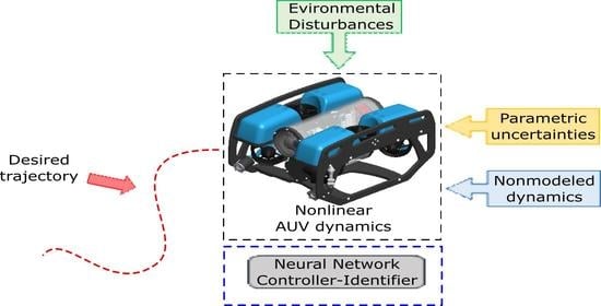The diagram in Figure 2 describes the general operation of the proposed algorithm applied to the AUV system dynamic Equations (20)–(23) for trajectory tracking. The closed-loop system structure is composed of the AUV dynamic model to develop a parallel identifier based on online adjustment of the DNN weights and the estimation law of parameter b, a reference system that generates the desired trajectory and a controller to calculate the input signal for both the AUV system and the identifier.

The DNCS scheme performs a simultaneous identification and control of the unknown perturbed AUV system, implementing an online training process that makes use of input–output data of its evolution over time. The learning laws that feed the proposed DNCS scheme comprise a set of differential equations for which the solutions are the DNN weight matrices and the parametric estimation of the constant input gain involved in the structure proposed in Equation (25). The DNN weight matrices $\mathit{W}\left(t\right)$ are updated according to the evolution over time of the identification error. This error is defined as the difference between the system and the identifier states. Additionally, the difference between the nominal and the actual values of these weight matrices is added, as a correction term (denoted by $\tilde{\mathit{W}}\left(t\right)$), in the adjustment of the learning law. On the other hand, the estimate $\widehat{b}\left(t\right)$ is also calculated by considering the identification error evolution to perform a parameter identification process. Thus, the DNCS-based identifier copies the system behavior by conducting an online adjustment of the weight matrices and the parametric estimate, causing the identification error to attain reduced values. The information provided by the identifier is used to design a tracking control for each AUV subsystem. This control input is comprised of the compensation of unknown dynamics of the plant provided by the DNCS and a standard feedback control.

Note for practitioners: the DNCS identification and control scheme carry out an online training process by using only the input–output information of the unknown perturbed AUV system. Regarding the DNCS algorithm tuning procedure, a set of parameters are adjusted by trial and error to perform effective identification and control of the unknown dynamics. The gain ${\gamma }_1$ determines the speed of learning of each DNN. This value is adjusted by taking into account the speed of the dynamic changes of the unknown AUV dynamics. That is, it takes greater values if the dynamic response to be identified is characterized by several signals of different frequencies (for example, hydrodynamic damping combined with abrupt currents or waves affecting the AUV system). Additionally, the nominal values of the weight matrices ${\mathit{W}}_{\mathit{0}}$ in the DNN structure can be adjusted. However, one may use their corresponding upper values, which may be supposed to be known, or they can be obtained by an offline training considering some AUV experimental data. The parameters $a_1$ and $a_2$ that correspond to the linear part of the DNN structure only must fulfill being negative real values, and generally, once they are selected, they are considered as fixed values. Another free design parameter is the adaptive gain ${\gamma }_2$, which is related to the rate of convergence of the parameter identification. Numerical simulations showed that the rate of parameter convergence increases with increasing adaptive gain. Regarding the sigmoidal activation function parameters ${\mathit{b}}_i$, ${\mathit{c}}_i$, and ${\mathit{d}}_i$, they can be selected by trial and error to enhance the identifier response; however, for simplicity in the simulation experiments, we considered some baseline values suggested by related works [39,54] that implements the kind of dynamic neural network used in the proposed DNCS.

6. Numerical Results

In this section, we present a set of two simulation results. The simulations were carried out by using the Matlab^® software environment. The first simulation consists of tracking the reference of an angular position for the yaw’s dynamic and a depth reference in the Z axis. In the second one, the underwater vehicle has the task of tracking a 3D helical trajectory with radius of 5 meters. In this simulation analysis, we present a comparison between the DNCS, a standard feedback controller designed by using Linear Quadratic Regulator (LQR) [55], and a Proportional Derivative (PD) controller implementing an online auto tuning method to set its parameters by using the successive approximation method (SAM) [56]. Hence, the self-tuned PD controller applies an adaptive approach to tackle the AUV control problem in order to perform a comparative performance analysis against the DNCS controller under fair conditions. Certainly, there exist other nonparametric control schemes or sliding mode techniques, which incorporates adaptive properties, that could be suitable alternatives for the system class subject of our analysis. However, a number of them need some gain adjustment, which is no longer required for the proposed DNCS controller. To conduct a more realistic simulation, in both scenarios, external disturbances were added to the dynamic model.

Table 1. Underwater vehicle parameters used in simulation.

Parameter	Value	Parameter	Value
$X_u$	$3.03\mathrm{kg}/\mathrm{s}$	$X_{\dot{u}}$	$5.5\mathrm{kg}$
$Y_v$	$3.21\mathrm{kg}/\mathrm{s}$	$Y_{\dot{v}}$	$12.7\mathrm{kg}$
$Z_w$	$8.18\mathrm{kg}/\mathrm{s}$	$Z_{\dot{w}}$	$14.57\mathrm{kg}$
$N_r$	$0.07\mathrm{kgm}/\mathrm{s}$	$N_{\dot{r}}$	$0.12{\mathrm{kgm}}^2$
$X_{u\left|u\right|}$	$4.03\mathrm{kg}/\mathrm{m}$	m	$11.5\mathrm{kg}$
$Y_{v\left|v\right|}$	$6.21\mathrm{kg}/\mathrm{m}$	W	$112.8\mathrm{N}$
$Z_{w\left|w\right|}$	$5.18\mathrm{kg}/\mathrm{m}$	B	$114.8\mathrm{N}$
$N_{r\left|r\right|}$	$0.07\mathrm{kgm}/\mathrm{s}$	$I_{zz}$	$0.16{\mathrm{kgm}}^2$

presents the parameters used for the dynamic model given in Equation (8). These parameters are taken from [57], derived by several experimental tests on the BlueROV2 vehicle [41]. These parameter values are also used for derivation of the referred LQR feedback controller. For the control strategy presented in Equation (42) and the adaptive laws given by Equations (46) and (47), the parameters used in the simulation are shown in

Table 2. Controller gains and adaptive law parameters used in the simulation results.

Parameters of the Controller and Adaptive Laws
Heading’s dynamic
$a_{{\psi }_1}=-28$	$a_{{\psi }_2}=-28$	$b_{\psi }\left(0\right)=30{\left({\mathrm{kgm}}^2\right)}^{-1}$
${\gamma }_{1,\psi }=20$	${\delta }_{W,\psi }=0.5$
${\gamma }_{2,\psi }=0.025$	${\delta }_{b,\psi }=0.05$
${\mathit{K}}_{\mathit{id},\mathit{\psi }}=[0.2,0.3]$	${\mathit{K}}_{\mathit{\psi }}=[120,80]$	${\mathit{P}}_{\mathit{2},\mathit{\psi }}=\mathrm{diag}\left([25,15]\right)$
${\mathit{W}}_{\mathit{0},\mathit{\psi }}=[5,5]$	${\mathit{W}}_{\mathit{\psi }}\left(0\right)=[0,0]$
Depth’s dynamic
$a_{z_1}=-2$	$a_{z_2}=-1$	$b_z\left(0\right)=-0.7{\mathrm{kg}}^{-1}$
${\gamma }_{1,z}=3$	${\delta }_{W,z}=0.5$
${\gamma }_{2,z}=0.04$	${\delta }_{b,z}=0.1$
${\mathit{K}}_{\mathit{id},\mathit{z}}=[0.2,0.1]$	${\mathit{K}}_{\mathit{z}}=[4,4]$	${\mathit{P}}_{\mathit{2},\mathit{z}}=\mathrm{diag}\left([27.5,16.5]\right)$
${\mathit{W}}_{\mathit{0},\mathit{z}}=[1.5,1]$	${\mathit{W}}_{\mathit{z}}\left(0\right)=[0,0]$
X-axis’ dynamic
$a_{x_1}=-0.0025$	$a_{x_2}=-0.005$	$b_x\left(0\right)=0.3{\mathrm{kg}}^{-1}$
${\gamma }_{1,x}=20$	${\delta }_{W,x}=2$
${\gamma }_{2,x}=0.00016$	${\delta }_{b,x}=0.6$
${\mathit{K}}_{\mathit{id},\mathit{x}}=[0.5,0.5]$	${\mathit{K}}_{\mathit{x}}=[6,4]$	${\mathit{P}}_{\mathit{2},\mathit{x}}=\mathrm{diag}\left([50,30]\right)$
${\mathit{W}}_{\mathit{0},\mathit{x}}=[0.2,0.1]$	${\mathit{W}}_{\mathit{x}}\left(0\right)=[0,0]$
Y-axis’ dynamic
$a_{y_1}=-0.25$	$a_{y_2}=-0.5$	$b_y\left(0\right)=-2{\mathrm{kg}}^{-1}$
${\gamma }_{1,y}=12$	${\delta }_{W,y}=1.5$
${\gamma }_{2,y}=0.00045$	${\delta }_{b,y}=0.05$
${\mathit{K}}_{\mathit{id},\mathit{y}}=[0.5,0.5]$	${\mathit{K}}_{\mathit{y}}=[8,7]$	${\mathit{P}}_{\mathit{2},\mathit{y}}=\mathrm{diag}\left([37.5,22.5]\right)$
${\mathit{W}}_{\mathit{0},\mathit{y}}=[0.2,0.1]$	${\mathit{W}}_{\mathit{y}}\left(0\right)=[0,0]$

.

It is worth mentioning that, for control purposes, the DNCS was developed based on the simplified dynamics given by Equations (21)–(23). However, it is important to stress that, in simulation experiments, we introduce the complete AUV 4DOF dynamical Equations (17)–(20) that considers a completely coupled AUV system (without any simplification). The simulation framework used in the experiments of the second scenario considers the four controllers (x, y, z, and yaw) acting at the same time. Implementation of the DNCS algorithm stabilizes to the yaw dynamic Equation (20), ensuring a fast controller response providing a rapid convergence to the origin. The previous action guarantees that the translational (x,y) dynamics in Equations (17) and (18) can be rapidly reduced to the ones described in Equations (21) and (22), simplifying the trigonometric coupling functions involving the yaw angle. Therefore, the DNCS algorithm is applied to the horizontal translational dynamic Equations (21) and (22) and for the z-axis dynamic Equation (23) separately to track desired 3D trajectories in the x-y-z space. However, the simulation were conducted by using the nominal model given by Equations (17) and (20).

In order to preserve the controllability condition for the estimated AUV system, it is necessary to guarantee the boundedness of $u\left(\xi \right)$ in Equation (42) by modifying the adaptive law Equation (47), so the estimates $\widehat{b}$ cannot reach values arbitrarily close or equal zero. In general, most of the parametric estimation problems provide some prior information about the localization of the parameter to be estimated. Such a prior information can be used to constrain or project the online estimation to remain in a known convex set. In our case, we need to constrain (project) the parametric estimate $\widehat{b}$ in a convex set to avoid the estimate taking values near to zero. One of the most common operators used in adaptive control systems is the so-called parameter projection operator [58]. For our case, we consider the following prior knowledge: the sign of b and the lower bound $b_0$ of the absolute value of b, i.e., $\left|b\right|\ge b_0$. This information can be obtained using the nominal parameter values of the added mass coefficients of the BlueROV2 vehicle structure, reported in [57]. Therefore, the restriction for the parameter estimate can be expressed as $|\widehat{b}|=\widehat{b}sgn\left(b\right)>b_0$. Now, following the procedure in [58], we can define the convex set where the parameter estimate must evolve, that is $S=\{\widehat{b}\in \mathbb{R}|b_0-\widehat{b}sgn\left(b\right)\le 0\}$. Therefore, we can apply the projection operator to the adaptive law:

$$\dot{\widehat{b}}\left(t\right)={\gamma }_2\left(2{\tilde{\mathit{\zeta }}}^{\top }{\mathit{P}}_{\mathit{2}}\mathit{B}u\left(\mathit{\zeta }\right)-{\delta }_b\widehat{b}\left(t\right)\right)=F\left(\tilde{\zeta }\right)$$

(52)

leading to

$$\dot{\widehat{b}}\left(t\right)=\mathit{Pr}\left(F\left(\tilde{\zeta }\right)\right)=\left\{\begin{array}{cc}F\left(\tilde{\zeta }\right),\hfill & \begin{array}{c}\mathrm{if}|\widehat{b}|>b_0\hfill \\ \mathrm{or}\mathrm{if}|\widehat{b}|=b_0\mathrm{and}{\tilde{\zeta }}^{\top }{\mathit{P}}_{\mathit{2}}\mathit{B}u\left(\zeta \right)sgn\left(b\right)>0,\hfill \end{array}\hfill \\ 0,\hfill & \mathrm{otherwise}\hfill \end{array}\right.$$

(53)

where $\widehat{b}\left(0\right)$ is chosen so that $\widehat{b}\left(0\right)sgn\left(b\right)>b_0$.

This modification constrains the parameter estimates inside some known convex bounded sets, which do not include zero. In other words, when the parameter $\widehat{b}$ reaches its lower absolute value $b_0$ and the time derivative $\widehat{b}$ is not zero, the adaption process is stopped. Moreover, by using the properties of the projection operator, the stability analysis developed in this research work holds [58].

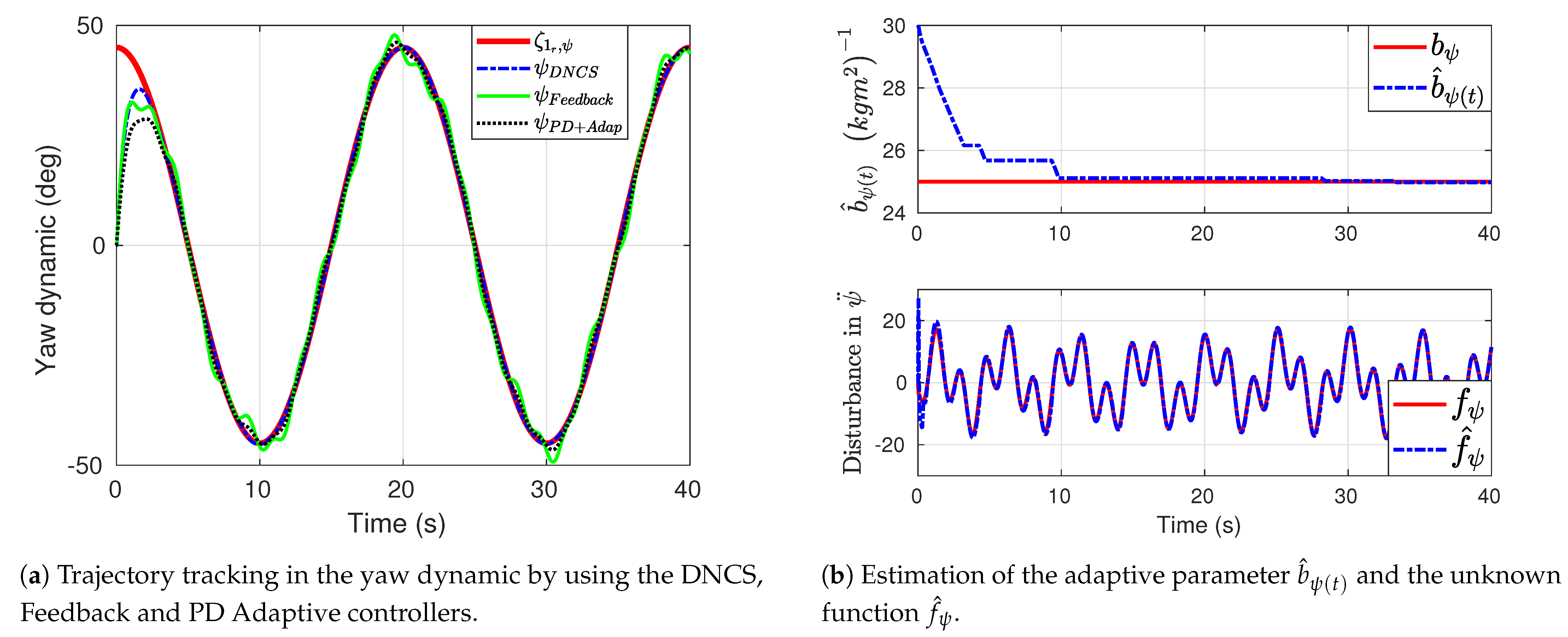
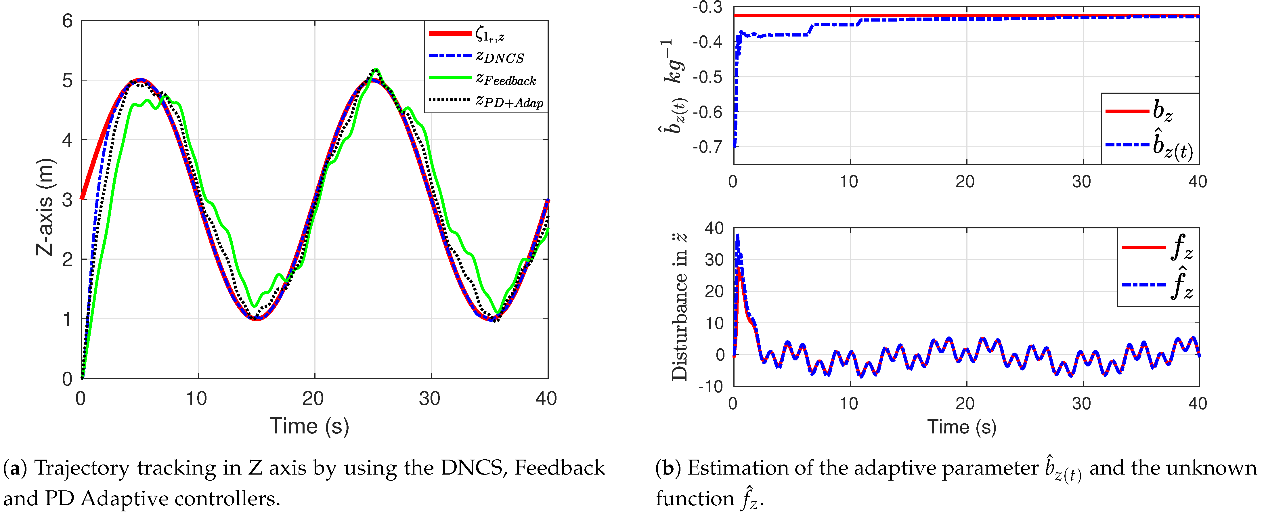
6.1. Yaw and Depth Trajectory Tracking

In this first simulation scenario, the underwater vehicle simultaneous maneuvers in the yaw and depth dynamics. The signal reference for yaw dynamic is a sine function with an amplitude of 45 degrees and a frequency of 0.1$\pi$ hertz given by

$$\begin{array}{cc}\hfill {\zeta }_{1_r,\psi }& =\frac{\pi }{4}cos\left(0.1\pi t\right)\hfill \\ \hfill {\zeta }_{2_r,\psi }& =-0.1\frac{{\pi }^2}{4}sin\left(0.1\pi t\right),\hfill \end{array}$$

(54)

and, for the Z axis, a sine function with an amplitude of 2 degrees and a frequency of 0.1$\pi$ hertz is chosen:

$$\begin{array}{cc}\hfill {\zeta }_{1_r,z}& =2sin\left(0.1\pi t\right)+3,\hfill \\ \hfill {\zeta }_{2_r,z}& =0.2\pi cos\left(0.1\pi t\right).\hfill \end{array}$$

(55)

In this scenario, the disturbance signals induced for the dynamic model (8) are given as

$$\begin{array}{cc}\hfill {\tau }_{{\psi }_d}=& 0.7sin\left(1.2t\right)cos\left(2.5t\right),\hfill \\ \hfill {\tau }_{z_d}=& 14cos\left(1.5t\right)sin\left(3t\right).\hfill \end{array}$$

(56)

In Figure 3 and Figure 4, we present the results obtained for the trajectory tracking problem in the yaw and depth dynamics. We can notice from Figure 3a and Figure 4a that the performance of the feedback controller is deteriorated as a consequence of unknown dynamics and the induced disturbances. In the case of the online tuned PD controller, it attains an improved tracking performance under the presence of unknown dynamics and disturbances due to its adaptive characteristics; however, the actual trajectory is still affected by oscillations around the reference signal. In contrast, the developed DNCS enables the system to track satisfactorily the reference signal, with a significantly less tracking error compared with the other controllers. The estimation of the lumped disturbances presented in Figure 3b and Figure 4b by using the dynamic neural network enables the DNCS to increase the performance of the underwater vehicle.

From Figure 3a and Figure 4a, we can observe that the parameters ${\widehat{b}}_{\psi }\left(t\right)$ and ${\widehat{b}}_z\left(t\right)$ converge to a small region in about 4 and 12 s, respectively. Additionally, we observe that the smaller the identification error of the parameters ${\widehat{b}}_{\psi }\left(t\right)$ and ${\widehat{b}}_z\left(t\right)$, the better approximation of the unknown dynamics ${\widehat{f}}_{\psi }$ and ${\widehat{f}}_z$ obtained. However, even when the adaptive parameters are far from their true value, the compensation of the dynamic neural network approximation enables us to conduct satisfactory trajectory tracking in the first seconds of the simulation, as can be observed in Figure 3 and Figure 4.

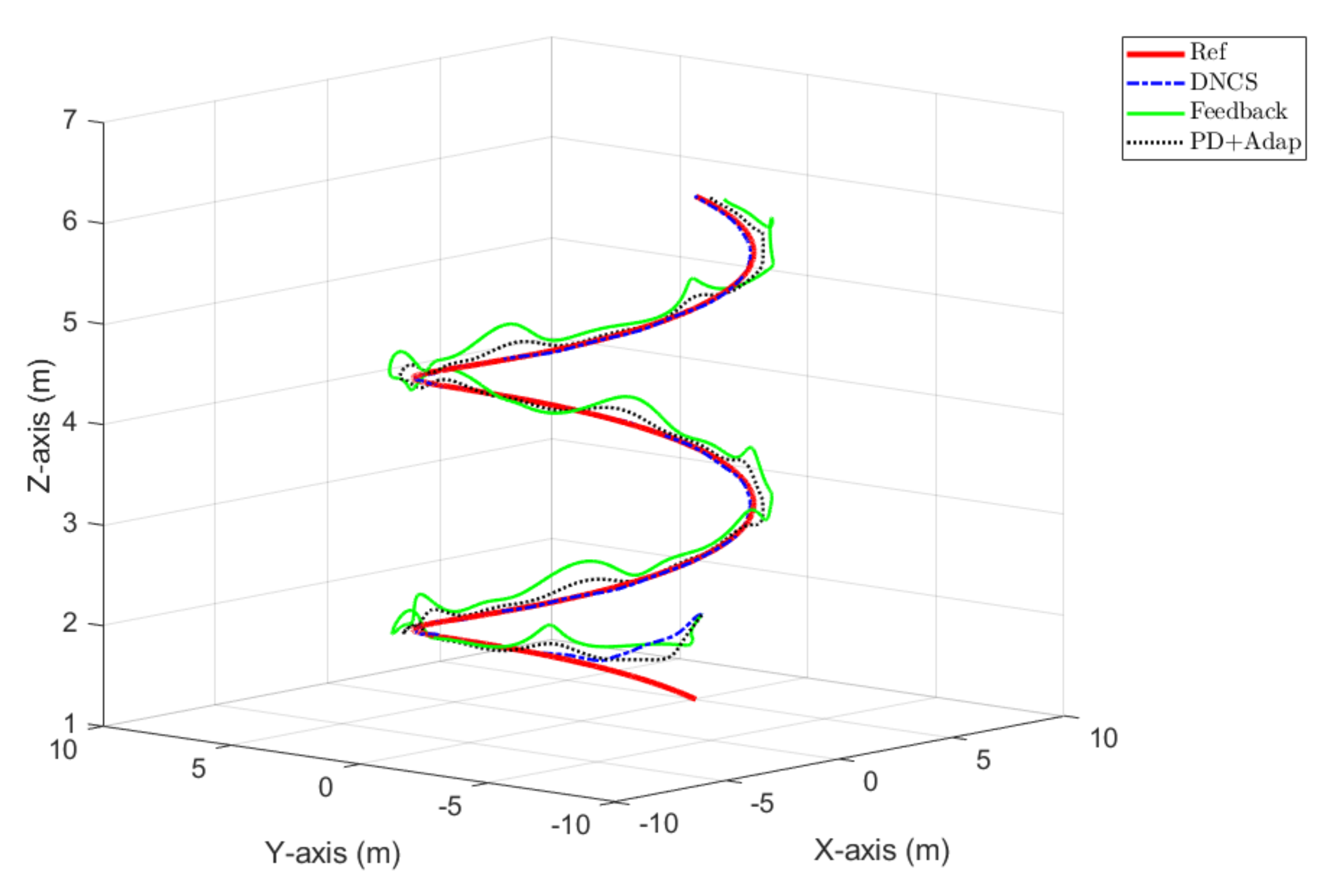
6.2. 3D Helical Trajectory Tracking

To verify the performance of the DNCS developed, a more complex scenario is proposed, where a 3D helical reference signal with a radius of 5 m is used. In this case, the desired signals for the X, Y, and Z axes are defined as

$$\begin{array}{cc}\hfill {\zeta }_{1_r,x}& =5cos\left(0.1\pi t\right),\hfill \\ \hfill {\zeta }_{2_r,x}& =-0.5\pi sin\left(0.1\pi t\right),\hfill \end{array}$$

(57)

$$\begin{array}{cc}\hfill {\zeta }_{1_r,y}& =5sin\left(0.1\pi t\right)\hfill \\ \hfill {\zeta }_{2_r,y}& =0.5\pi cos\left(0.1\pi t\right),\hfill \end{array}$$

(58)

$$\begin{array}{cc}\hfill {\zeta }_{1_r,z}& =\frac{1}{8}t+1\hfill \\ \hfill {\zeta }_{2_r,z}& =\frac{1}{8}.\hfill \end{array}$$

(59)

In the same way as in Section 6.1, disturbance signals were added to the dynamic model (8) for the 3D helical desired trajectory, which are given as

$$\begin{array}{cc}\hfill {\tau }_{x_d}=& 15sin\left(1.2t\right)cos\left(1.5t\right),\hfill \\ \hfill {\tau }_{y_d}=& 10cos\left(2t\right)sin\left(0.5t\right),\hfill \\ \hfill {\tau }_{z_d}=& 10cos\left(t\right)sin\left(3t\right).\hfill \end{array}$$

(60)

The simulation results for the 3D helical trajectory tracking scenario are shown in Figure 5, Figure 6, Figure 7 and Figure 8. Figure 5 depicts three-dimensional trajectory tracking with respect to the reference trajectory, which shows the accomplishment of the tracking mission. In this simulation experiment, the yaw angle desired is selected as 0 radians. The initial position for the AUV is selected as $\left(x\left(0\right),y\left(0\right),z\left(0\right)\right)=\left(3,-2,2\right)$. The 3D trajectory begins at a depth of 2 m, reaching up to 6 meters, with the center at the origin and a radius of 5 meters. This kind of trajectory can be useful in 3D reconstruction applications of underwater structures. We can observe the trajectory tracking results for both controllers: DNCS and the feedback controller. Notice that the feedback controller is not able to counteract the effects caused by the lumped disturbances, whereas the DNCS enables the AUV to track the desired 3D trajectory with a small tracking error.

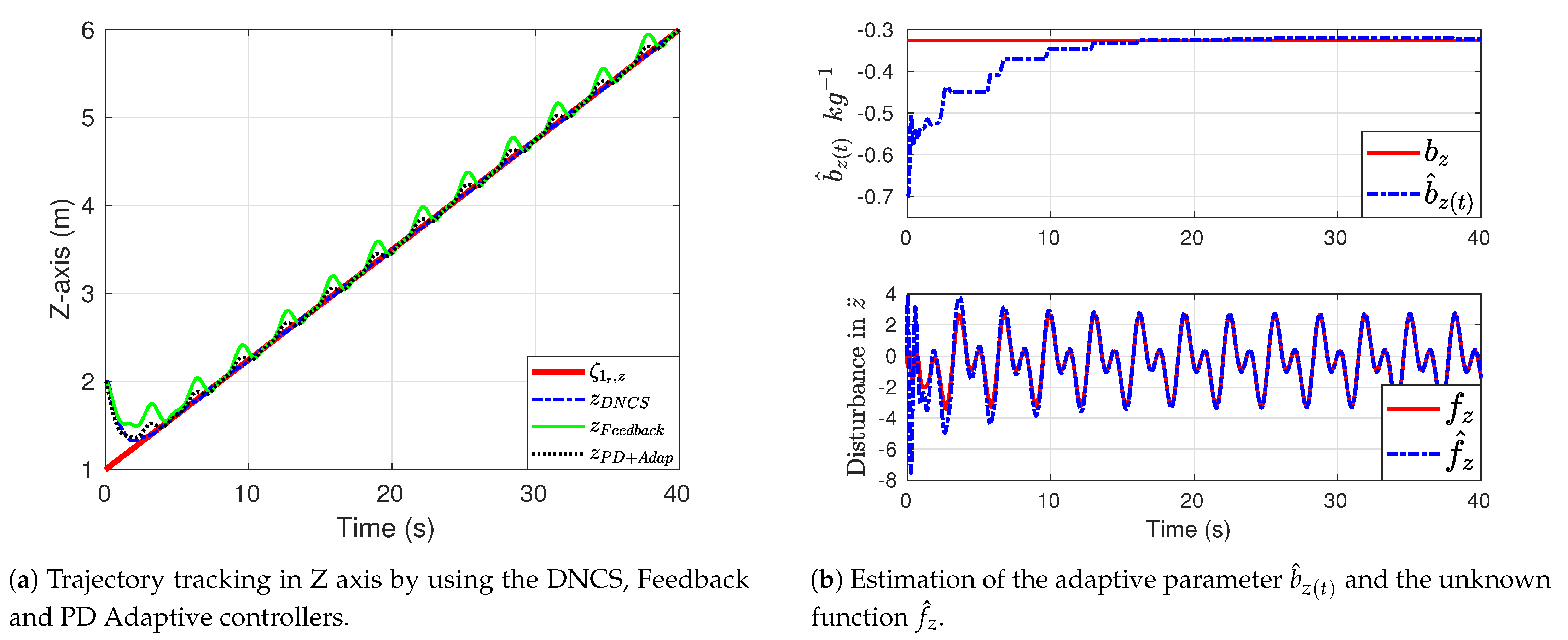
Figure 6a, Figure 7a, and Figure 8a illustrate the time evolution of the position of the underwater vehicle in the X, Y, and Z axes. In the three axes are presented the performance of the DNCS; the feedback controller; and the PD controller, which implements a self-tuning process. When the dynamic neural network is added to the feedback controller, performance is significantly increased, reducing the tracking error and enabling the AUV to track the desired reference without abrupt changes. In the case of the PD controller that implements an online parameter adjustment, the deviation with respect to the desired trajectory is reduced; however, this type of controller fails to eliminate oscillations of the system trajectory.

The time evolution of the adaptive parameters ${\widehat{b}}_x\left(t\right)$, ${\widehat{b}}_y\left(t\right)$, and ${\widehat{b}}_z\left(t\right)$ is presented in Figure 6b, Figure 7b, and Figure 8b, respectively. These parameters converge from the initial value to a small bounded region in approximately 15 s in all the cases. The importance of the estimation of the adaptive parameters should be recalled because it enables the UAV to track a desired references without the knowledge of any parameter of the dynamic model Equations (17)–(20).

In Figure 6b, Figure 7b, and Figure 8b, the estimation of the unknown functions $f_x$, $f_y$ and $f_z$, the so-called lumped disturbances, is presented. After the first 10 s of simulation, one can appreciate that the identifier based on the DNCS estimates in a satisfactory way the unknown dynamics and the external disturbances. Moreover, the identification error converges to the compact residual set around zero given by Equation (48). Additionally, a performance index analysis is conducted to compare both DNCS and feedback controllers. The comparison were performed by the following two quality indexes for the tracking error:

$$J_{IAE}\left(T\right)={\int }_0^T\left|e_1\left(t\right)\right|dt,$$

(61)

$$J_{ISE}\left(T\right)={\int }_0^T{e}_1^2\left(t\right)dt,$$

(62)

and the following two indexes for the identification error:

$$J_{STD}\left(T\right)=\sqrt{\frac{1}{T}{\int }_0^T{({\tilde{\zeta }}_1\left(t\right)-{\overline{\tilde{\zeta }}}_1)}^{2}dt},$$

(63)

where ${\overline{\tilde{\zeta }}}_1$ denotes the mean value of the set of identification error values.

$$J_{RMSE}\left(T\right)=\sqrt{\frac{1}{T}{\int }_0^T{\tilde{\zeta }}_1^2\left(t\right)dt},$$

(64)

The performance index proposed in Equation (61) is given by the Integral of Absolute Error (IAE) to measure the absolute tracking deviation. The second index in Equation (62) is defined by the Integral of Squared Error (ISE) to quantify the absolute squared tracking deviation. The index given in Equation (63) is the standard deviation used to measure the dispersion of the identification error produced by the DNCS scheme. Additionally, the performance index (64) is defined as the root mean square error (RMSE) of the identification error. This is used to measure the amount of error between the set of values of the system and the identifier states. The proposed comparison analysis reports that applying the DNCS controller and the feedback controller solves the trajectory tracking.

Table 3. Performance index comparison for yaw and depth trajectory tracking.

Dynamic	Controller	IAE	ISE
Yaw angle	DNCS	$117.4$	$42.0$
	PD+Adap	$285.9$	$48.7$
	Feedback	$391.0$	$57.3$
Z axis	DNCS	$703.7$	$1288.3$
	PD+Adap	$2085.5$	$1867.9$
	Feedback	$4140.5$	$4369.4$

and

Table 4. Performance index comparison for 3D helical trajectory tracking.

Dynamic	Controller	IAE	ISE
X axis	DNCS	$855.5$	$679.1$
	PD+Adap	$1774.6$	$905.5$
	Feedback	$3268.5$	$2059.4$
Y axis	DNCS	$750.8$	$523.5$
	PD+Adap	$3168.2$	$2048.9$
	Feedback	$6446.6$	$7003.2$
Z axis	DNCS	$239.1$	$122.7$
	PD+Adap	$428.5$	$154.6$
	Feedback	$846.8$	$245.6$

show the calculated values for $J_{IAE}$ and $J_{ISE}$ (considering $T=40\mathrm{s}$), with the tracking error data involving the two proposed scenarios. This quantitative comparison validates the argument concerning the advantage of using the proposed DNCS-based controller. The numerical data presented in Table 3 and Table 4 demonstrate that the proposed DNCS-based controller yields the smallest tracking error of $J_{IAE}$ and $J_{ISE}$; this means that the AUV tracks the reference trajectories with a superior performance. This evaluation intends to highlight the benefit for the application of the suggested controller in contrast with the feedback controller to regulate AUVs when the dynamic model information is incomplete.

The information in

Table 5. Performance index comparison for yaw and depth identification.

Dynamic	RMSE	Std Deviation
Yaw angle	$0.0725$	$0.0713$
Z axis	$0.4013$	$0.3932$

and

Table 6. Performance index comparison for 3D helical identification.

Dynamic	RMSE	Std Deviation
X axis	$0.2913$	$0.2846$
Y axis	$0.2558$	$0.2525$
Z axis	$0.1239$	$0.1215$

shows numerical data of $J_{STD}$ and $J_{RMSE}$ for both experiments considering $T=40\mathrm{s}$. The reported small standard deviation values indicate that the identification error at every step tends to be near the mean value of each set of error values (for each dynamic). In other words, the values of the identification errors have uniform behavior, avoiding abrupt changes or dispersion when they evolve over time. On the other hand, the small numerical values for the RMSE index evidence the fact that each DNCS estimate remains close to its corresponding subsystem trajectory during the simulation time. This validation seems to justify implementation of the proposed DNCS controller for identifying the closed loop AUV subsystems.

Remark 1.

The DNCS algorithm was designed with the aim to provide a low computational complexity solution considering the notion of a lightweight algorithm, which allows an eventual onboard implementation in a small experimental platform. In this sense, the 4DOF AUV mathematical model is represented by four second-order equations, which are rewritten in their corresponding integrator chain representation. Thus, each second-order system is characterized by two first-order differential equations. The latter aims to avoid matrix operations (nested for loops, which may increment the computational time). Additionally, the right-hand sides of the learning law for the DNN weight matrix $W\left(t\right)$ and the adaptive law for $b\left(t\right)$ were decomposed in simple arithmetic operations. Hence, the closed loop system simulation of the DNCS control algorithm and the complete AUV model is comprised of several simulation steps, but it intends to be computationally efficient since it uses simple calculations. This fact makes it a conservative algorithm without any major impact to system performance.

7. Conclusions

In this research work, a novel Dynamic Neural Control System (DNCS) was developed to solve the trajectory tracking problem for an autonomous underwater vehicle with 4DOF in the presence of unmodeled dynamics, parametric uncertainties, and unknown external disturbances. A proof based on a proposed Lyapunov function candidate to demonstrate the closed-loop stability was derived. The stability formal result establishes sufficient conditions in order to guarantee the ultimate boundedness of the identification and tracking errors. These conditions involve the solution of a set of two AREs, a specific control law structure, and certain adaptive laws for the synaptic weights and for the estimate of the unknown input parameter. Besides solving the trajectory tracking problem, the proposed DNCS lets us estimate and compensate (a) unmodeled dynamics and external disturbances and (b) uncertain constant gains that multiply the control signal. The main strength of the proposed control strategy consists of solving the trajectory tracking problem with reduced knowledge of the mathematical model of the AUV (basically a reduced structure) but without any knowledge of the system parameters. A set of simulations were conducted in order to demonstrate the effectiveness and applicability of the proposed methodology. Moreover, a comparison analysis via two performance indexes of the DNCS with respect to a feedback controller and a self-tuned PD controller both without a dynamic neural compensation and a parameter estimation were also conducted. These comparisons show that the proposed DNCS technique is more effective in dealing with unmodeled dynamics, parameter uncertainties, and external disturbances. The identification capacity of the DNCS to approximate the highly nonlinear behavior of the AUV is validated in the different scenarios presented in the numerical experiments. Furthermore, the simulations also showed that the tracking and identification errors are ultimately bounded and remain in a compact residual set around zero. Furthermore, two additional performance indexes were used to measure the performance of the identification process of the AUV system through the standard deviation and RMSE criterions, reaching the conclusion that the DNCS identifier possesses great properties dealing with modeling a and parametric uncertainties. Future research directions consider the implementation of the control strategy developed in at least two underwater vehicle platforms with different characteristics to verify the performance in real-time and under unknown environments. Moreover, if we consider the more general case where the added mass terms are wave frequency-dependent as considered in hydrodynamic theory, the assumption in the mathematical model that the parameter b remains constant is unsatisfied. Hence, the DNCS developed can be extended to estimate time-varying parameters, adding for example another dynamic neural network for this purpose.

References

1. Fossen, T.I. Guidance and Control of Ocean Vehicles; John Wiley & Sons: Chichester, UK, 1994; ISBN 0-471-94113-1. [Google Scholar]
2. Graver, J.G. Underwater Gliders: Dynamics, Control and Design. Ph.D. Thesis, Princeton University, Princeton, NJ, USA, 2005. [Google Scholar]
3. Wadoo, S.; Kachroo, P. Autonomous Underwater Vehicles: Modeling, Control Design and Simulation; CRC Press: Boca Raton, FL, USA, 2017. [Google Scholar]
4. Cely, J.S.; Saltaren, R.; Portilla, G.; Yakrangi, O.; Rodriguez-Barroso, A. Experimental and Computational Methodology for the Determination of Hydrodynamic Coefficients Based on Free Decay Test: Application to Conception and Control of Underwater Robots. Sensors 2019, 19, 3631. [Google Scholar] [CrossRef] [Green Version]
5. Morrison, A.; Yoerger, D.R. Determination of the hydrodynamic parameters of an underwater vehicle during small scale, nonuniform, 1-dimensional translation. In Proceedings of the OCEANS’93, Victoria, BC, Canada, 18–21 October 1993; pp. II277–II282. [Google Scholar]
6. Velasco, F.J.; Herrero, E.R.; Santos, F.J.L.; Rodríguez, J.M.R.; Hernández, J.J.D.; Antolín, L.M.V. Measurements of Hydrodynamic Parameters and control of an underwater torpedo-shaped vehicle. IFAC Pap. 2015, 48, 167–172. [Google Scholar] [CrossRef]
7. Jagadeesh, P.; Murali, K.; Idichandy, V. Experimental investigation of hydrodynamic force coefficients over AUV hull form. Ocean Eng. 2009, 36, 113–118. [Google Scholar] [CrossRef]
8. Nouri, N.; Mostafapour, K.; Bahadori, R. An apparatus to estimate the hydrodynamic coefficients of autonomous underwater vehicles using water tunnel testing. Rev. Sci. Instruments 2016, 87, 065106. [Google Scholar] [CrossRef] [PubMed]
9. Li, Z.; Tao, J.; Sun, H.; Luo, Y.; Ding, L.; Deng, Z. Hydrodynamic calculation and analysis of a complex-shaped underwater robot based on computational fluid dynamics and prototype test. Adv. Mech. Eng. 2017, 9, 1687814017734500. [Google Scholar] [CrossRef] [Green Version]
10. Castillo-Zamora, J.J.; Camarillo-Gómez, K.A.; Pérez-Soto, G.I.; Rodríguez-Reséndiz, J.; Morales-Hernández, L.A. Mini-AUV Hydrodynamic Parameters Identification via CFD Simulations and Their Application on Control Performance Evaluation. Sensors 2021, 21, 820. [Google Scholar] [CrossRef]
11. Tang, S.; Ura, T.; Nakatani, T.; Thornton, B.; Jiang, T. Estimation of the hydrodynamic coefficients of the complex-shaped autonomous underwater vehicle TUNA-SAND. J. Mar. Sci. Technol. 2009, 14, 373–386. [Google Scholar] [CrossRef]
12. Cardenas, P.; de Barros, E.A. Estimation of AUV hydrodynamic coefficients using analytical and system identification approaches. IEEE J. Ocean. Eng. 2019, 45, 1157–1176. [Google Scholar] [CrossRef]
13. Kepler, M.E.; Pawar, S.; Stilwell, D.J.; Brizzolara, S.; Neu, W.L. Assessment of AUV Hydrodynamic Coefficients from Analytic and Semi-Empirical Methods. In Proceedings of the OCEANS 2018 MTS/IEEE Charleston, Charleston, SC, USA, 22–25 October 2018; pp. 1–9. [Google Scholar]
14. Conte, G.; Zanoli, S.; Scaradozzi, D.; Gambella, L. Evaluation of Hydrodynamics Parameters of a UUV. In Proceedings of the IWUR 2005, International Workshop On Underwater Robotics For Sustainable Management Of Marine Ecosystem And Environmental Monitoring, Genoa, Italy, 9–11 November 2005. [Google Scholar]
15. Tiwari, B.K.; Sharma, R. Design and Analysis of a Variable Buoyancy System for Efficient Hovering Control of Underwater Vehicles with State Feedback Controller. J. Mar. Sci. Eng. 2020, 8, 263. [Google Scholar] [CrossRef] [Green Version]
16. Bi, A.; Zhao, F.; Zhang, X.; Ge, T. Combined Depth Control Strategy for Low-Speed and Long-Range Autonomous Underwater Vehicles. J. Mar. Sci. Eng. 2020, 8, 181. [Google Scholar] [CrossRef] [Green Version]
17. Sun, Y.; Zhang, C.; Zhang, G.; Xu, H.; Ran, X. Three-Dimensional Path Tracking Control of Autonomous Underwater Vehicle Based on Deep Reinforcement Learning. J. Mar. Sci. Eng. 2019, 7, 443. [Google Scholar] [CrossRef] [Green Version]
18. Sun, Y.; Ran, X.; Zhang, G.; Xu, H.; Wang, X. AUV 3D Path Planning Based on the Improved Hierarchical Deep Q Network. J. Mar. Sci. Eng. 2020, 8, 145. [Google Scholar] [CrossRef] [Green Version]
19. Szymak, P.; Małecki, J. Control System of Underwater Vehicle Based on Artificial Intelligence Methods. In Automation and Robotics; BoD—Books on Demand: Norderstedt, Germany, 2008; pp. 285–296. [Google Scholar]
20. Pshikhopov, V.; Chernukhin, Y.; Guzik, V.; Medvedev, M.; Gurenko, B.; Piavchenko, A.; Saprikin, R.; Pereversev, V.; Krukhmalev, V. Implementation of intelligent control system for autonomous underwater vehicle. Appl. Mech. Mater. 2015, 701, 704–710. [Google Scholar] [CrossRef]
21. Shi, Y.; Qian, W.; Yan, W.; Li, J. Adaptive depth control for autonomous underwater vehicles based on feedforward neural networks. In Intelligent Control and Automation; Springer: Berlin/Heisenberg, Germany, 2006; pp. 207–218. [Google Scholar]
22. Chen, S.; Lin, T.; Jheng, K.; Wu, C. Application of Fuzzy Theory and Optimum Computing to the Obstacle Avoidance Control of Unmanned Underwater Vehicles. Appl. Sci. 2020, 10, 6105. [Google Scholar] [CrossRef]
23. Trslić, P.; Omerdic, E.; Dooly, G.; Toal, D. Neuro-Fuzzy Dynamic Position Prediction for Autonomous Work-Class ROV Docking. Sensors 2020, 20, 693. [Google Scholar] [CrossRef] [PubMed] [Green Version]
24. Lorentz, J.; Yuh, J. A survey and experimental study of neural network AUV control. In Proceedings of the Symposium on Autonomous Underwater Vehicle Technolog, Monterey, CA, USA, 2–6 June 1996; pp. 109–116. [Google Scholar]
25. Van de Ven, P.; Flanagan, C.; Toal, D. A Survey of AI Techniques for Control of Underwater Vehicles. IFAC Proc. Vol. 2003, 36, 145–150. [Google Scholar] [CrossRef]
26. Che, G.; Yu, Z. Neural-network estimators based fault-tolerant tracking control for AUV via ADP with rudders faults and ocean current disturbance. Neurocomputing 2020, 411, 442–454. [Google Scholar] [CrossRef]
27. Huang, H.; Li, J.; Zhang, G.; Tang, Q.; Wan, L. Adaptive recurrent neural network motion control for observation class remotely operated vehicle manipulator system with modeling uncertainty. Adv. Mech. Eng. 2018, 10, 1687814018804098. [Google Scholar] [CrossRef]
28. Wang, J.; Wang, C.; Wei, Y.; Zhang, C. Command filter based adaptive neural trajectory tracking control of an underactuated underwater vehicle in three-dimensional space. Ocean. Eng. 2019, 180, 175–186. [Google Scholar] [CrossRef]
29. Ma, Z.; Hu, J.; Feng, J.; Liu, A. Diving adaptive position tracking control for underwater vehicles. IEEE Access 2019, 7, 24602–24610. [Google Scholar] [CrossRef]
30. Xia, Y.; Xu, K.; Li, Y.; Xu, G.; Xiang, X. Adaptive trajectory tracking control of a cable-driven underwater vehicle on a tension leg platform. IEEE Access 2019, 7, 35512–35531. [Google Scholar] [CrossRef]
31. Avelar, A.; Salgado, I.; Ahmed, H.; Mera, M.; Chairez, I. Differential neural networks observer for second order systems with sampled and quantized output. IFAC Pap. 2018, 51, 490–495. [Google Scholar] [CrossRef]
32. García-González, A.; Poznyak, A.; Chairez, I.; Tatyana, P. Differential Neural Networks Observers: Development, Stability Analysis and Implementation. In Systems Structure and Control; IntechOpen: London, UK, 2008; Chapter 3; pp. 61–82. [Google Scholar] [CrossRef] [Green Version]
33. García, A.; Chairez, I.; Poznyak, A. Hybrid differential neural network identifier for partially uncertain hybrid systems. In Recent Advances in Intelligent Control Systems; Springer: Berlin/Heisenberg, Germany, 2009; pp. 149–168. [Google Scholar]
34. Cervantes-Rojas, J.S.; Muñoz, F.; Chairez, I.; González-Hernández, I.; Salazar, S. Adaptive tracking control of an unmanned aerial system based on a dynamic neural-fuzzy disturbance estimator. ISA Trans. 2020. [Google Scholar] [CrossRef]
35. Yu, W.; Poznyak, A. Indirect adaptive control via parallel dynamic neural networks. IEE Proc. Control. Theory Appl. 1999, 146, 25–30. [Google Scholar] [CrossRef]
36. Chaudhuri, T.; Soh, Y.C.; Li, H.; Xie, L. A feedforward neural network based indoor-climate control framework for thermal comfort and energy saving in buildings. Appl. Energy 2019, 248, 44–53. [Google Scholar] [CrossRef]
37. He, W.; Yan, Z.; Sun, C.; Chen, Y. Adaptive neural network control of a flapping wing micro aerial vehicle with disturbance observer. IEEE Trans. Cybern. 2017, 47, 3452–3465. [Google Scholar] [CrossRef]
38. Asl, H.J.; Narikiyo, T.; Kawanishi, M. Neural network-based bounded control of robotic exoskeletons without velocity measurements. Control. Eng. Pract. 2018, 80, 94–104. [Google Scholar]
39. Poznyak, A.S.; Sanchez, E.N.; Yu, W. Differential Neural Networks for Robust Nonlinear Control: Identification, State Estimation and Trajectory Tracking; World Scientific: Singapore, 2001. [Google Scholar]
40. García, E.; Murano, D.A. Differential neural networks for identification and filtering in nonlinear dynamic games. Math. Probl. Eng. 2014, 2014, 306761. [Google Scholar] [CrossRef] [Green Version]
41. Blue Robotics Inc. Available online: https://bluerobotics.com/ (accessed on 25 January 2021).
42. Fuentes-Aguilar, R.Q.; Chairez, I. Adaptive Tracking Control of State Constraint Systems Based on Differential Neural Networks: A Barrier Lyapunov Function Approach. IEEE Trans. Neural Networks Learn. Syst. 2020, 31, 5390–5401. [Google Scholar] [CrossRef]
43. Ballesteros, M.; Polyakov, A.; Efimov, D.; Chairez, I.; Poznyak, A. Differential neural network identification for homogeneous dynamical systems. IFAC Pap. 2019, 52, 233–238. [Google Scholar] [CrossRef]
44. Mitrinovic, D.S.; Pecaric, J.; Fink, A.M. Classical and New Inequalities in Analysis; Springer: Berlin/Heisenberg, Germany, 2013; Volume 61. [Google Scholar]
45. Poznyak, A. Advanced Mathematical Tools for Control Engineers: Volume 1: Deterministic Systems; Elsevier: Amsterdam, The Netherlands, 2010; Volume 1. [Google Scholar]
46. Fossen, T.I. Marine Control Systems-Guidance. Navigation, and Control of Ships, Rigs and Underwater Vehicles; Marine Cybernetics: Trondheim, Norway, 2002. [Google Scholar]
47. Fossen, T.I. Handbook of Marine Craft Hydrodynamics and Motion Control; John Wiley & Sons: Hoboken, NJ, USA, 2011. [Google Scholar]
48. Garcia, P.C.; Lozano, R.; Dzul, A.E. Modelling and Control of Mini-Flying Machines; Springer: Berlin/Heisenberg, Germany, 2006. [Google Scholar]
49. Carrillo, L.R.G.; López, A.E.D.; Lozano, R.; Pégard, C. Modeling the quad-rotor mini-rotorcraft. In Quad Rotorcraft Control; Springer: Berlin/Heisenberg, Germany, 2013; pp. 23–34. [Google Scholar]
50. Rangel, M.A.G.; Manzanilla, A.; Suarez, A.E.Z.; Muñoz, F.; Salazar, S.; Lozano, R. Adaptive non-singular terminal sliding mode control for an unmanned underwater vehicle: Real-time experiments. Int. J. Control. Autom. Syst. 2020, 18, 615–628. [Google Scholar] [CrossRef]
51. Ljung, L. System identification. In Wiley Encyclopedia of Electrical and Electronics Engineering; John Wiley & Sons: Hoboken, NJ, USA, 1999; pp. 1–19. [Google Scholar]
52. Poznyak, A.; Escobar, J.; Shtessel, Y. Stochastic sliding modes identification. In Proceedings of the InternationalWorkshop on Variable Structure Systems, VSS’06, Alghero, Italy, 5–7 June 2006; pp. 226–231. [Google Scholar]
53. Khalil, H.K. Nonlinear Systems; Prentice Hall: Upper Saddle River, NJ, USA, 2002; Volume 3. [Google Scholar]
54. Salgado, I.; Chairez, I. Adaptive unknown input estimation by sliding modes and differential neural network observer. IEEE Trans. Neural Netw. Learn. Syst. 2017, 29, 3499–3509. [Google Scholar] [PubMed]
55. Al Makdah, A.A.R.; Daher, N.; Asmar, D.; Shammas, E. Three-dimensional trajectory tracking of a hybrid autonomous underwater vehicle in the presence of underwater current. Ocean. Eng. 2019, 185, 115–132. [Google Scholar] [CrossRef]
56. Gade, S.; Shendage, S.; Uplane, M. On line auto tuning of PID controller using successive approximation method. In Proceedings of the 2010 International Conference on Recent Trends in Information, Telecommunication and Computing, Kochi, India, 12–13 March 2010; pp. 277–280. [Google Scholar]
57. Sandøy, S.S. System Identification and State Estimation for Rov Udrone. Master’s Thesis, NTNU, Trondheim, Norway, 2016. [Google Scholar]
58. Ioannou, P.; Fidan, B. Adaptive Control Tutorial; SIAM: Philadelphia, PA, USA, 2006. [Google Scholar]
Figure 1. Reference frames: inertial (red) and body-fixed (blue).
Applsci 11 02797 g001
Figure 2. Block diagram of the closed-loop system.
Applsci 11 02797 g002
Figure 3. Simulation results for trajectory tracking in yaw dynamic.
Applsci 11 02797 g003
Figure 4. Simulation results for trajectory tracking in Z axis.
Applsci 11 02797 g004
Figure 5. Underwater vehicle response in a 3D helical desired trajectory scenario by using the DNCS, Feedback and PD Adaptive controllers.
Applsci 11 02797 g005
Figure 6. Simulation results for trajectory tracking of a 3D helical reference signal in the X axis.
Applsci 11 02797 g006
Figure 7. Simulation results for trajectory tracking of a 3D helical reference signal in Y axis.
Applsci 11 02797 g007
Figure 8. Simulation results for trajectory tracking of a 3D helical reference signal in Z axis.
Applsci 11 02797 g008