Article

Generating Synthetic Fermentation Data of Shindari, a Traditional Jeju Beverage, Using Multiple Imputation Ensemble and Generative Adversarial Networks

Department of Computer Engineering, Jeju National University, 102 Jejudaehak-ro, Jeju-si 63243, Korea
*
Author to whom correspondence should be addressed.
Appl. Sci. 2021, 11(6), 2787; https://doi.org/10.3390/app11062787
Submission received: 8 February 2021 / Revised: 15 March 2021 / Accepted: 16 March 2021 / Published: 20 March 2021
(This article belongs to the Special Issue Generative Models in Artificial Intelligence and Their Applications)

Abstract

:
Fermentation is an age-old technique used to preserve food by restoring proper microbial balance. Boiled barley and nuruk are fermented for a short period to produce Shindari, a traditional beverage for the people of Jeju, South Korea. Shindari has been proven to be a drink of multiple health benefits if fermented for an optimal period. It is necessary to predict the ideal fermentation time required by each microbial community to keep the advantages of the microorganisms produced by the fermentation process in Shindari intact and to eliminate contamination. Prediction through machine learning requires past data but the process of obtaining fermentation data of Shindari is time consuming, expensive, and not easily available. Therefore, there is a need to generate synthetic fermentation data to explore various benefits of the drink and to reduce any risk from overfermentation. In this paper, we propose a model that takes incomplete tabular fermentation data of Shindari as input and uses multiple imputation ensemble (MIE) and generative adversarial networks (GAN) to generate synthetic fermentation data that can be later used for prediction and microbial spoilage control. For multiple imputation, we used multivariate imputation by chained equations and random forest imputation, and ensembling was done using the bagging and stacking method. For generating synthetic data, we remodeled the tabular GAN with skip connections and adapted the architecture of Wasserstein GAN with gradient penalty. We compared the performance of our model with other imputation and ensemble models using various evaluation metrics and visual representations. Our GAN model could overcome the mode collapse problem and converged at a faster rate than existing GAN models for synthetic data generation. Experiment results show that our proposed model executes with less error, is more accurate, and generates significantly better synthetic fermentation data compared to other models.

1. Introduction

Shindari is a traditional Jeju beverage made out of rice or barley and manufactured through a fermentation process that takes 3–4 days in summer and 5–7 days in winter [1]. Shindari is considered a Jeju yogurt and also known as sweet liquor or low-alcohol wine. Jeju is a volcanic island and, in older days, it was difficult to transport and acquire food from the mainland, so the only way to obtain food was to rely on ingredients produced on the island itself and by preserving food through fermentation. To produce Shindari, barley is first cleaned, dried, grounded, and kneed to form the shape. Then, the barley is fermented at 40 degrees Celsius and can be stored for 2 months.
Fermented foods are of great consumer acceptability and nutritional value. Fermented food, especially yogurt, helps to reinstate proper microbial balance in the intestine, helping in the elimination of lactose intolerance, thus improving the overall immune system. Research has also shown [2] that fermented food can recover people from Hepatitis C and liver problems. Along with all these advantages, there are threats if the fermentation process is overdone or if the microbial organisms are not fermented for the optimal period, causing contamination. In 2001, there was an outbreak of botulism contamination in Alaska that triggered many people to be hospitalized after taking food fermented for an improper amount of time [3]. People suffered from heart attacks and many required a tracheostomy to keep them alive. Therefore, there is a need to find the optimal fermentation time for each microbial community so that they have maximum productivity towards benefiting human health and not adversely affecting mankind. Predicting the ideal time for fermentation depending on various external conditions like temperature, pH, humidity, etc., requires past observed data. For Shindari, there is a lack of experimentation data of the microbial community and it is also not easily accessible. So, predicting microbial spoilage to eliminate any adverse effect of the fermentation process of Shindari is a necessary and complicated task.
Synthetic data has been generated mostly for medical data using generative adversarial networks. In [4], a generative adversarial networks (GAN) framework is applied to generate artificial EEG signals that are mostly available as tabular data. Mostly, autoregressive models such as waveGAN are used for generating time series data [5]. However, a regular CNN model is used for better interpretability instead of autoregressive models in the proposed EEG–GAN model.
Past work has additionally used generative models for the motivations behind making additional training data. In the realm of computer vision, a previous study [6] presented a GAN model that learns to improve the realism of synthetic tagged images using real, unlabeled images. The generator input is a synthetic image and the output is a refined image. The discriminator must learn to classify images as real or refined. They show that the improved realism enables training of better models for gaze and hand pose estimation by adding refined tagged images to the training set. The ECG heart rate classification task [6] similarly demonstrated that classification performance could be improved by adding synthetic ECG heartbeats generated from a standard GAN to a training set. It also generates synthetic ECG signals that can be used in training; however, unlike the previous work, we use a simulator to improve the deep generative model’s ability to generate synthetic labeled ECG heartbeats that have tabular data.
Another recent study proposed DoseGAN [7], which is an attention-gated GAN model. This is proposed to increase the complexity of the model, improve model learning, and increase the complexity of the model. It also aims to reduce network redundancy by focusing on relevant anatomy. Classical methods of classification at the level of ECG beats focused on extracting interval characteristics and using previous knowledge of the morphology of the ECG [8]. Each ECG signal is separated into heartbeats using heartbeat detection techniques [9]. For each heartbeat, the characteristics related to heartbeat intervals and ECG morphology are calculated, then the combined characteristics are introduced in supervised machine learning models based on linear discriminants (LD) [10]. The application of deep learning models to ECG classification has become popular and has been applied to many tasks, such as arrhythmia detection at the cardiologist level [11] and classification of ECG heartbeats [12,13,14,15].
The state-of-the-art method for classifying EKG heartbeat levels [14] has recently shown that superior results are achieved when applying the ResNet convolution model that classifies each heartbeat class separately in this work to the training of such deep learning systems that have been trained with additional synthetic EKG heartbeats generated from the previously proposed generative models. medGAN (medical generative adversarial networks) is a well-known tool for constructing practical synthetic medical records. They combine autoencoders and GAN architecture to produce high-dimensional discrete values [16]. The authors used autoencoders in medGAN to delegate samples to learn outstanding features. GAN was equipped with previously qualified autoencoders to produce distributed patient data instead of directly generating patient records. Synthetic healthcare data has also been collected using generative adversarial networks [17]. To capture the connection between consecutive diagnostic data, the authors used one-dimensional (1-D) convolutional neural networks. Convolutional autoencoders were then used to connect discrete and continuous values. PATE (Private Aggregation of Teacher Ensembles) is another GAN model for generating synthetic data that preserves the generator’s differential privacy, which is critical for biomedical data [18]. The generator in PATE–GAN is similar to that of a regular GAN model, but the discriminator is fitted with a PATE mechanism, resulting in K-teacher discriminators and asymmetrical training. Pedro Narvaez et al. [19] used GAN to synthesize natural heart sounds. Neuron-based generative models for SSVEP classification in EEG data is one of the models [20]. For this, the researchers used deep convolutional generative adversarial networks and variational autoencoders. Using the bidirectional recurrent neural network, recent work has also yielded efficient results for producing single synthetic biomedicals [21].
Synthetic data are artificial data generated by replicating the statistical characteristics of the original data. There are many methods of generating synthetic data. When real data is not available, synthetic data can be created according to distribution known by the data analyst or the best-fit distribution can be determined for the original data. Variational autoencoder and generative adversarial networks are the latest models that perform superior to traditional models in generating synthetic data. The synthetic data generated through deep learning models are processed through classification, clustering, and regression algorithms to validate their correlation with the original data and evaluate how they impact the performance and accuracy of the models when compared to using original data. Often, original data has missing values that, when imputed, play an important role in enhancing the performance of any model. Prediction of missing values in original data is one of the most important tasks and the initial task for generating synthetic data. In this paper, we propose multiple imputation ensemble to predict the missing values in the original data and then apply generative adversarial networks to generate synthetic fermentation data for Shindari from the original tabular data. The main contribution of this paper is summarized below:
  • In the preprocessing stage, we proposed a multiple imputation model which is a combination of multivariate imputation by chained equations (MICE) and random forest imputation model (RFI) to impute the original missing data.
  • Multiple imputation was then combined with the bagging and stacking ensemble approach to predict and complete the tabular fermentation data.
  • We proposed tabular GAN with skip connection and adapted WGAN–GP architecture to generate synthetic tabular data. We proposed TGAN-skip–WGAN-GP (Tabular GAN-skip with Wasserstein GAN with gradient penalty), which could enhance the performance by reducing convergence time and eliminating the mode collapse problem.
  • In the evaluation stage, we visually and quantitatively produced the performance of the proposed imputation and GAN model.
  • The proposed approach can be utilized for generating synthetic data for any kind of fermentation process that involves tabular data.
We present the outcome of our proposed approach in the Results section. Imputation with ensemble was evaluated mean dissimilarity, regressor accuracy, and Kappa error plots. GAN was evaluated through correlation coefficient, mean absolute error, root mean square error, percent root mean square difference, Fréchet Distance, and mirror column association.

2. Proposed Methodology for Generating Synthetic Fermentation Data of Shindari

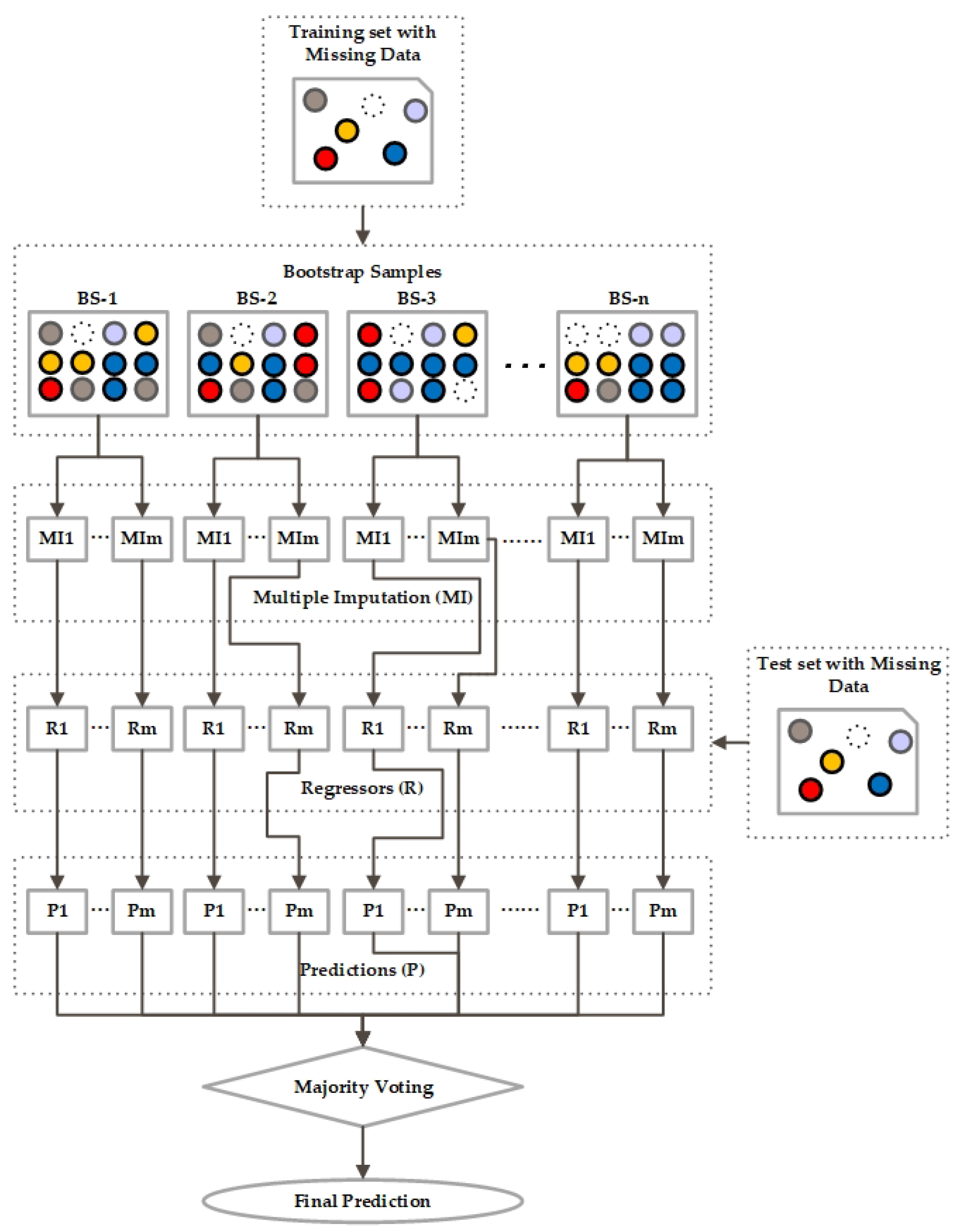
In this section, we elaborate on our proposed approach for generating synthetic fermentation data of Shindari using the multiple imputation ensemble method and generative adversarial networks. The overview of the proposed approach is presented in Figure 1. First, we discuss the data we used for the implementation and then proceed with the explanation of preprocessing, prediction, and GAN synthesizer stage. In the preprocessing phase, the distribution of unknown data is used by the multiple imputation method to fill up the missing values of the fermentation dataset. For the multiple imputation approach, we explored several imputation methods, among which multivariate imputation by chained equations (MICE) and random forest imputation (RFI) executed plausible results. The bagging and stacking ensemble approach was used to aggregate the predictions of various regressors to obtain best predictions to feed the GAN synthesizer. After the final prediction, the proposed method transforms the data, applies TGAN–skip–WGAN–GP architecture to synthesize the tabular data, performs inverse transformation, and produces the end result for synthetic fermentation data generation of Shindari. We evaluated our proposed architecture based on the output quality of imputation and synthetic data.
This section is further divided into four subsections that explain the overall approach used for each module in the proposed architecture. Shindari microbial community data is described in Section 2.1, we explain preprocessing of the data in Section 2.2, the next Section 2.3 presents the methodology we have used for prediction, and finally, we define the GAN architecture for generating synthetic data in Section 2.4.

2.1. Shindari Microbial Community Data

It is also important to understand how our data was obtained, factors influencing the fermentation process, the variety of raw materials used, and the interaction between microbial communities. The Shindari fermentation extract was prepared by combining cooked rice, barley nuruk, and water, which was left in a 30 C incubator and was sampled for 24 h, 72 h, or 120 h. The samples were then filtered and 99% ethanol was added to balance the final concentration to 70%. Fermented beverages contain microorganisms that interact with other microorganisms to form a community and each community represents different characteristics. Therefore, it is important to analyze the microbial community and their interaction rather than focus only on individual microorganisms. At every stage of the fermentation process, the changes in the microbial community were observed. While obtaining the Shindari data for our experiment, it was found that different fermentation times had different effects on the microbial community structures. It was found that lactic acid bacteria was over 97% when the samples were fermented for over 3 days. For example, within 24 h of fermentation, Saccharomyces cerevisiae is mainly involved in the Shindari fermentation process where it produces ethanol, carbon dioxide, and other compounds from sugars in the rice, whereas Pediococcus sp.—which enhances immunity and prevents the growth of several spoilage and pathogenic microorganisms—is rapidly dominant during 48 h to 72 h of the fermentation process. When we synthesize to generate new data, we consider the combinations of microorganisms and their interaction and learn the distribution of microorganisms for each specific microbial community from the original data. The detailed procedure to obtain our data can be reviewed from [1]. We present the layout of our data in Figure 2.
The microbial community CSV data of Shindari was obtained from the Jeju Inside Agency & Cosmetic Science Center, Republic of Korea [1]. Features of our interest among many from the CSV data were rank, taxonomy, name of the microbial community, and the total count for each community. We had only species in the rank category, whereas taxonomy in the CSV data represented the grouping of microorganisms having the same characteristics. The name feature defined names of the Shindari microbial community. Each species and microbial community contained several microorganisms. During the fermentation process, the composition of every microbial community changes. According to the experimentation in laboratories, we could obtain total counts for each microbial community for the 1st, 3rd, 5th, and 7th day. For our research work to generate synthetic data, we considered the top ten most relevant and important microbial communities in the fermentation process of Shindari [1]. They are, namely, Bacillus amyloliquefaciens group, Citrobacter koseri, Enterobacter asburiae group, Enterococcus durans group, Escherichia hermannii group, Lactococcus lactis group, Pantoea allii, Pediococcus acidilacticici group, Pediococcus_uc, and Ralstonia pickettii. Rank; taxonomy; name; and total count for the 1st day, 3rd, 5th, and 7th day of each microbial community from the Shindari fermentation data is then passed through the preprocessing, prediction, and GAN synthesizer stages to obtain the new data.

2.2. Preprocessing

The raw data has the total count for the alternate days of the week but lacks hourly information, which would make the generation of synthetic data more correlated to the original data. Therefore, in the preprocessing stage, we take the training set with missing data and perform multiple imputation. There are four different approaches to handle missing data [22]. An overall analysis can be done to deal with missing data, statistical imputation methods and imputation using machine learning algorithms are also well-known approaches. Another way is by creating an algorithm that can itself incorporate the mechanism to deal with missing data. In our proposed work, we concentrate on two different multiple imputation techniques, namely, multivariate imputation by chained equations (MICE) and random forest imputation (RFI).

2.2.1. Multivariate Imputation by Chained Equations

Multivariate Imputation by Chained Equations is based on Fully Conditional Specification (FCS), which defines multivariate imputation method with conditional densities for each incomplete variable one after the other. Let us assume that I n , where ( n = 1 , 2 , , m ) is one of the incomplete variables, where I = ( I 1 , I 2 , , I m ) . We denote the observed and missing values in I as I n O = ( I 1 O , , I m O ) and I n M i s = ( I 1 M i s , , I m M i s ) , respectively. Q u a n t represents the quantity of scientific interest, which is often a multivariate vector [23]. So, with the above notation, the main steps of MICE can be explained as below:
  • We start the experimentation by analyzing the observed incomplete data I O . To estimate Q u a n t from I O , we need to make assumptions from the unobserved data. From the distribution of observed data, we select related or plausible values to replace the missing values. For each column or variable with missing values I M i s s , MICE identifies an imputation model and iterates repeatedly based on the number of variables or columns with missing values.
  • For each imputed dataset, we then compute the Q u a n t with an identical model.
  • The last step involves pooling of all the Q u a n t estimates into one Q u a n t and evaluating its variance. The missing values are either replaced by predictions of the model or by using mean matching.

2.2.2. Random Forest Imputation

We use random forest imputation since it requires less hyperparameter tuning, is inexpensive in measuring Out of Bag (OOB) performance and is efficient in handling nonlinear relationships in data. In the random forest approach, we use the proximity imputation method to fill the missing values. The missing values are divided according to continuous and categorical variables. For continuous variables, the imputation is done using the median of nonmissing values; for categorical variables, frequently existing nonmissing values are used for imputation. The imputed data is utilized to fit a random forest, which is used to determine the symmetric proximity matrix. We then use the proximity matrix to fill the original missing values. We use the weighted mean of nonmissing data to fill the missing values of continuous variables and over nonmissing data, the largest mean proximity is used to fill the missing values of categorical variables [24]. After every iteration, a new random forest is generated and the process is repeated.

2.3. Ensemble and Prediction

Ensemble was introduced by Tukey [25] to combine several base models of machine learning to find an optimal model for prediction. The ensemble technique can be used for both classification and regression tasks. In our work, instead of using a single model, we induced a set of regressors and aggregated their prediction to obtain a better result. Ensemble techniques can be categorized into homogeneous and heterogeneous types. Homogeneous, as the name suggests, are ensembles that are created from regressors of the same type, whereas heterogeneous defines ensembles created by combining regressors of different types. Our main goal of using the ensemble model is to achieve higher accuracy and better performance compared to any single model. In our proposed work, we achieve this by using the bagging and stacking ensemble.

2.3.1. Bagging Ensemble

Bagging is a well-known ensemble approach useful for both classification and regression problems. Bagging is also known as “bootstrap aggregating”. Bootstrapping refers to the generation of bootstrap samples of size B S from a dataset of size D S , using random selections from B S observations. These samples are mostly obtained from the unknown data distribution and from each other or independently. These are further used for variance approximation of the estimator. For every model, there is an input, output, and processing layer. The processing of the model used for a particular problem differs according to the input training dataset and so does the output, according to the performance of each model. Bagging is the process where we apply and try to fit various independent models and, at the end, average their prediction to obtain the best result with low variance.
As shown in Figure 3, the first step in bagging approach is that we create multiple B S , then we fit a base regressor for each B S and aggregate them to obtain the average of their outputs. Let us denote m bootstrap samples of size B S as in (1):
{ O 1 1 , O 2 1 , , O B S 1 } , { O 1 2 , O 2 2 , , O B S 2 } , , { O 1 m , O 2 n , , O B S m } ,
where O r p is the rth observation of pth bootstrap sample. Therefore, there can be n independent base regressors { R 1 , R 2 , , R m } , as shown in Figure 3. Then, to obtain the ensemble model, we combine and compute the average of the regressor to get a model with a lower variance. The average can be denoted as in Equation (2):
A v g m = 1 m p = 1 m O p .
Every regressor model makes a prediction and after majority voting, the final prediction is the one that receives more than half of the vote.

2.3.2. Stacking Ensemble

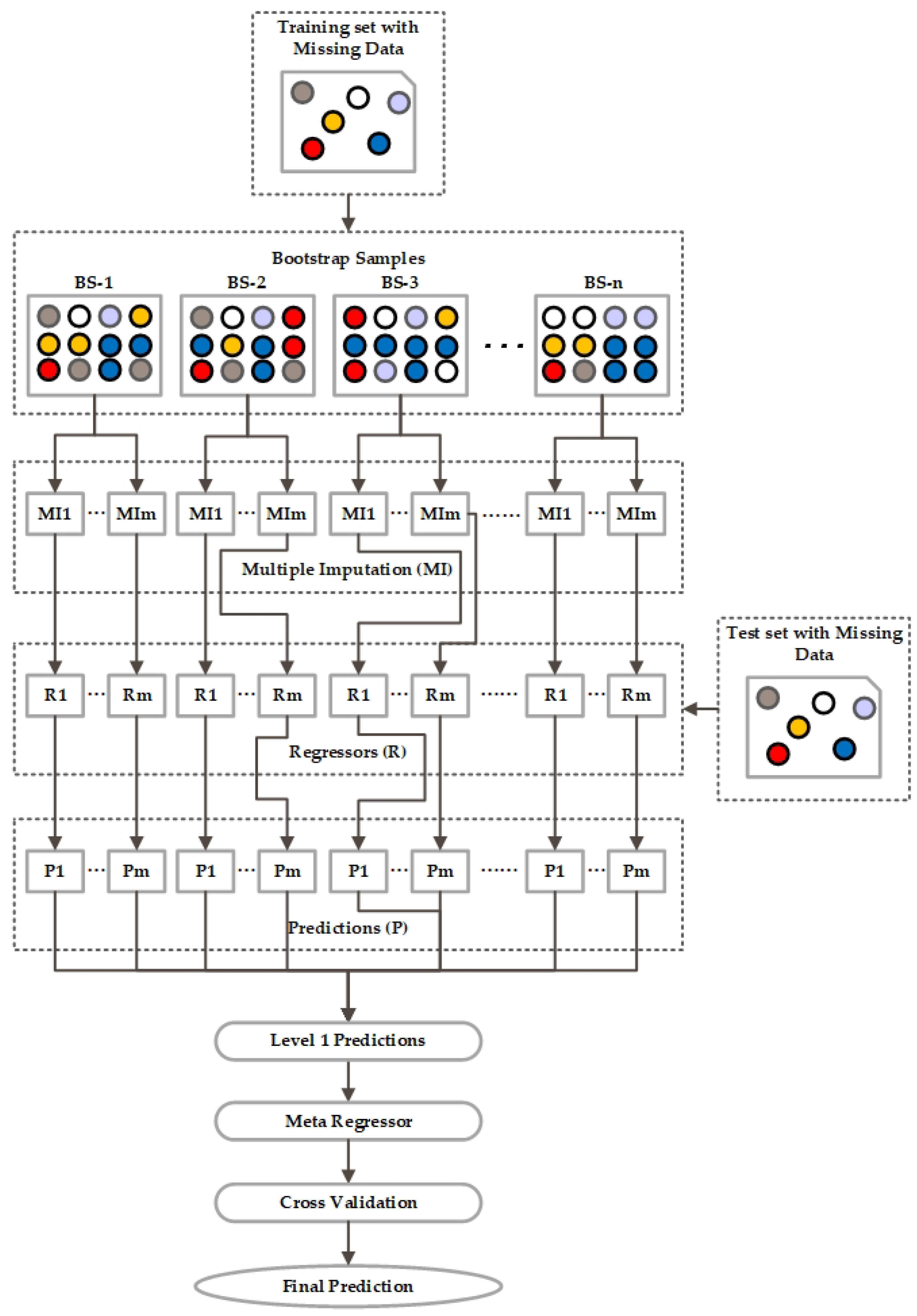
The next ensemble model is the stacking ensemble, which combines several base learners by training a metamodel and uses the output of the regressors instead of the training input data to develop the ensemble model [26]. So, to build a stacking ensemble, we first produced the models by training a set of base learners on the full training input data. The prediction from the first layer of each model is used as an input or metalevel attribute to the ensemble model. As we can see from Figure 4, the new set of predictions at level 1 is used to train a meta regressor in the ensemble model. After cross-validation, we obtain the final prediction.

2.4. Generative Adversarial Networks for Generating Synthetic Fermentation Data for Shindari

2.4.1. Overview

Generative Adversarial Networks were first introduced by Ian Goodfellow et al. [27] in the year 2014 as a machine learning framework where two neural network competes against each other in a zero-sum game. GAN is considered as one of the cutting edge frameworks that can be effectively applied in various fields, producing incredible results. The two networks in the GAN model are known as the generator network ( G ) and discriminator network ( D ) . As shown in Figure 5, random input noise variable Z p ( p ) is first passed through the generator network that retains the data distribution D p d over data x. The discriminator is fed with the samples generated from the generator and the real data. The discriminator then attempts to evaluate and correctly distinguish between the sample from the generator and the real data. The goal of the GAN architecture is that the generator continuously tries to fool the discriminator and at one point it becomes successful in generating realistic samples that cannot be distinguished from the real data. So, the generator tries to minimize l o g ( 1 D ( G ( p ) ) ) and the minmax game function can be defined as in Equation (3):
min G max D F ( D , G ) = E x D p d ( x ) [ l o g D ( x ) ] + E p Z p ( p ) [ l o g ( 1 D ( G ( p ) ) ) ] .
In this paper, we propose a combination resulting in an improved version of the well-known GAN model to generate synthetic tabular data related to the fermentation of Shindari. The architectures involved in the proposed methodology are as follows:
  • Improved version of Tabular GAN (TGAN) with skip connections [28];
  • Enhancing TGAN-skip with WGAN-GP (Wasserstein GAN with gradient penalty architecture.
Therefore, we combine these architectures to form TGAN-skip–WGAN-GP for generating synthetic data. We first preprocess the data by removing unwanted data and perform data transformation to make sense of the continuous and categorical values. After the transformation, we pass the data through our GAN model (TGAN-skip–WGAN-GP). The output data from the GAN model goes through a reverse transformation and finally generates the synthetic data, which is then evaluated.

2.4.2. Data Transformation

A significant representation of the original data is required for any machine learning model to extract meaningful data. Data transformation of continuous values is commonly done through normalization or standardization. Normalization is the process where the values are transformed between 0 and 1, whereas in standardization, the data is transformed to have a mean value of 0 and standard deviation of 1. We performed standardization with the real data x, which can be defined as in (4), where λ is the mean and σ is the standard deviation.
x ¯ = x λ σ .
For categorical values, we used embedding for data transformation. Embedding conserves the semantic relationship by transforming large vectors into smaller dimensional space vectors.

2.4.3. TGAN-Skip–WGAN-GP

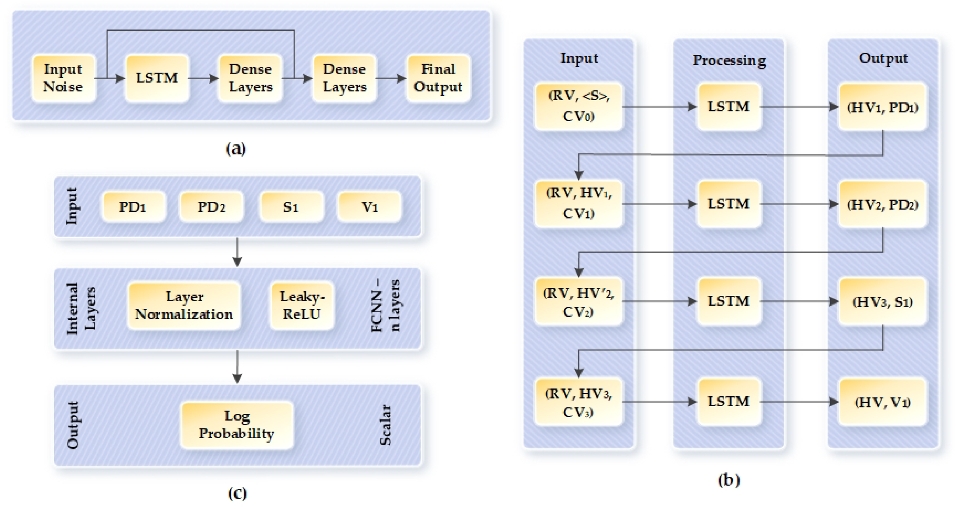
TGAN is a general purpose GAN for generating synthetic data for tabular datasets. In general, the TGAN architecture does not possess skip connections. We use the improved version of TGAN that has skip connections to eliminate the vanishing gradient problem and decrease the convergence time with improvements in the overall performance. The skip connections in the TGAN architecture preserve the high magnitude of activation by allowing prompt activation to skip in-between layers. This results in retaining old information, achieves higher gradients, and helps in training deeper models [28]. Figure 6a depicts the layout of the TGAN-skip architecture. For the generator of the GAN architecture, we used the long short-term memory (LSTM) cell, as shown in Figure 6b, and the discriminator is built with multilayer perceptron (MLP), as shown in Figure 6c. The generator is modeled to generate each continuous variable in two steps and each categorical variable in one step. For continuous variables, we first generate the value scalar S n and then the cluster vector V n ; for categorical variables, we compute the probability distribution P D n over each label, as shown in Figure 6b. R V is the random variable that is forwarded as input to the LSTM cell in each step s t along with the previous hidden vector H V n or embedding vector H V n and the attention-based context vector C V n [29]. We can determine the context from the attention weight vector β s t by Equation (5):
β s t = p = 1 s t exp β s t , p q exp β s t , q O u t p ,
where O u t is the output from the LSTM cell. In TGAN, the output from the LSTM passes through two dense layers to generate the final output, then the output of the two dense layers goes through another dense layer to form the attention vector for the next iteration of the LSTM network. We added the skip connection in between the two dense layers.
WGAN [30] was built to solve the flaws in Vanilla GAN. WGAN-GP, developed by Gulrajani et al. [31], proposed an improved version of WGAN by introducing a gradient penalty that eliminates the need for clipping and complies with the constraint of 1-Lipschitz. The new objective or loss by WGAN-GP is defined by the combination of the original critic loss and gradient penalty loss, as mentioned in Equations (6) and (7):
O r i g i n a l C r i t i c L o s s = E x ˜ G p [ l o g D ( x ˜ ) ] E x ^ R p [ D ( x ) ] ,
G r a d i e n t P e n a l t y L o s s = λ E x ^ P x ^ [ ( x ^ D ( x ^ ) 2 1 ) 2 ] ,
where R p and G p are the data and generator distribution with x ^ P x ^ denoting random samples. The value of λ , according to [31], is selected as 10 since when experimented, it worked well with various datasets and architectures. Using the WGAN-GP architecture for TGAN-skip decreases the discriminator loss and improves the performance of the generator. Normally, TGAN uses the architecture of vanilla GAN, in which any imbalance between the generator and discriminator can cause stagnation of training. By using WGAN-GP architecture in the TGAN-skip model, we can avoid a stagnation scenario and mode collapse. TGAN-skip–WGAN-GP also converges smoothly with higher speed than the TGAN with vanilla GAN architecture. To implement the WGAN-GP architecture in TGAN-skip, we adapted the loss function to the Wasserstein distance and evaluated the gradient penalty. We changed the batch normalization layer of the discriminator in TGAN-skip to layer normalization and eliminated the sigmoid activation from the last layer. Furthermore, according to WGAN-GP architecture, we trained the discriminator for more iterations compared to the generator.
For the discriminator, as shown in Figure 6c, we use n fully connected neural network layers and, for input, we combine P D i , S i and V i . Then, the internal layers of the discriminator were computed through (8):
H V i ( D ) = L e a k y R e L U ( L a y e r N o r m ( L P i D ( H V i 1 D d i v e r s i t y ( H V i 1 D ) ) ) ) , i = 2 : n ,
where L a y e r N o r m is layer normalization in the discriminator, L P is the learning parameter, ⊕ represents concatenation, and d i v e r s i t y defines the minibatch vector of the discriminator.

2.4.4. Inverse Transformation

Since the data was transformed to generate more meaning, it is required to perform inverse transformation with respect to the initial data transformation to obtain an output as realistic as the original input data. We can convert the continuous data into a scalar that ranges from −1 to 1 along with a multinomial distribution, and discrete variables are also converted into a multinomial distribution. The synthetic data generated for Shindari fermentation is then evaluated to measure the correlation with the original data and to evaluate our proposed model.

3. Results and Discussion

We evaluated our model based on the quality of multiple imputation ensemble method results and synthetic data generated by the GAN model. The evaluation metrics we used to judge imputation results are mean dissimilarity, regressor accuracy, and Kappa error plots. For the GAN model, we evaluated mean correlation coefficient, mean absolute error, root mean square error, percent root mean square difference, Fréchet distance, and mirror column association. In Section 3.1 and Section 3.2, we show the results of our experimentation for imputation and generation of synthetic data.

3.1. Imputation

For evaluating our imputation method, we experimented and compared the results of different combinations of imputation and ensemble methods, as shown in Table 1. As regressors, we compared the outcome of using support vector (SV), decision tree (DT), random forest (RF), and simple linear (SL) regressors, in different multiple imputation ensemble model. Values marked as bold in Table 1 performed better than other regressors and, from the result, we can say that random forest produces the best result and the combination of imputation and ensemble mentioned in our proposed work (RFI-Bag, RFI-SE, MICE-Bag, and MICE-SE) performed better than other approaches. In Table 1, “Bag” represents bagging ensemble and “SE” denotes stacking ensemble.

3.1.1. Mean Dissimilarity

To measure mean dissimilarity between the imputed and original data, we used the normalized Euclidean distance. The closer the value of mean dissimilarity to zero, the better the quality of imputed data. Table 1 shows random forest imputation separately, with bagging and stacking ensembles producing values closer to zero indicating better performance.

3.1.2. Kappa Error Plots

Kappa error plots identify a point for every regressor in the ensemble model to measure the diversity-error pattern for the ensemble model [32]. So, the lesser the error, the better the model’s performance. So, according to the results shown in Table 1, RFI-SE produces less error than other models.

3.1.3. Original Data

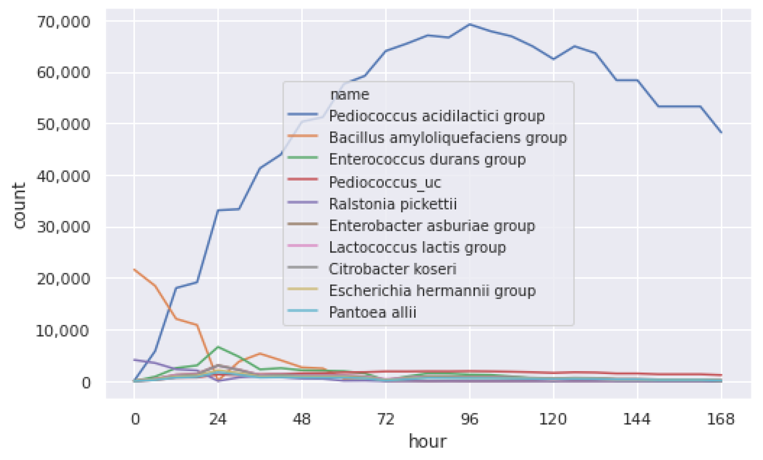
Figure 7 shows the count distribution of the ten microbial communities that are most relevant in Shindari fermentation. Original data refers to the raw data we obtained from the Cosmetic Science Center. The count is for 1st, 3rd, 5th, and 7th day and, as we can see from the figure, the fermentation process makes the counts of the microbial community change continuously.

3.1.4. Imputed Data

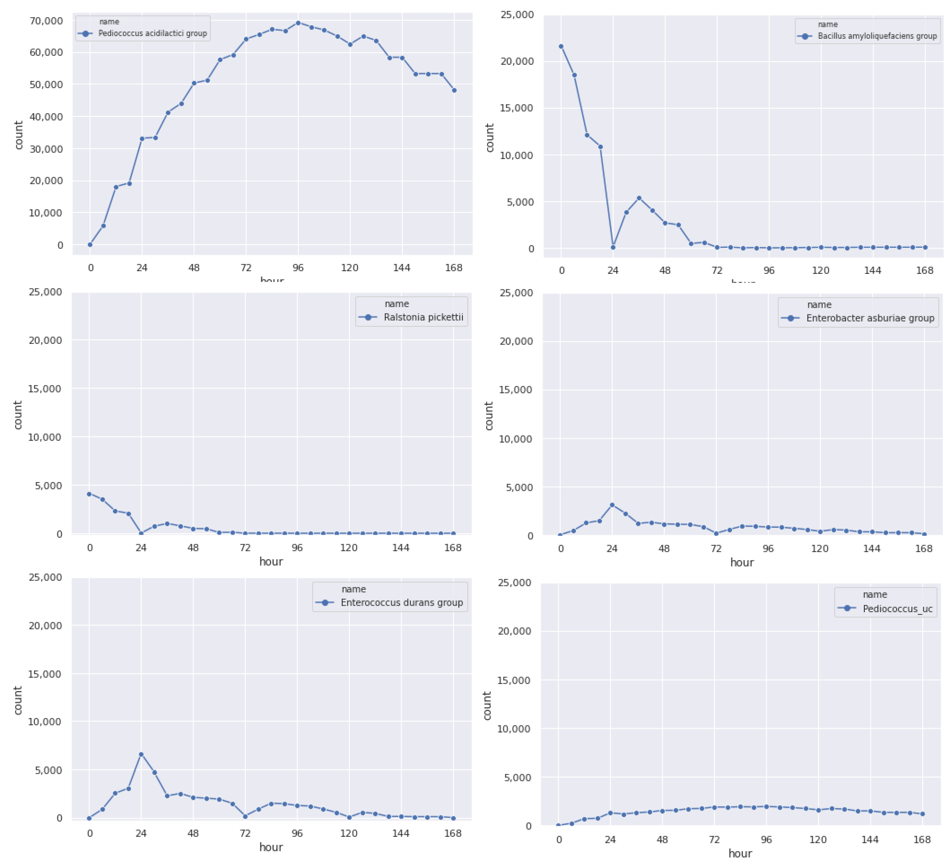
The original data is then imputed to fill the missing values. We generated six-hour data for every microbial community, as shown in Figure 8. We show the imputation result for different microbial communities in Figure 9. Comparing Figure 9 with the original data in Figure 7, we can see that the imputed value is correlated with the original count distribution of each microbial community.

3.2. Synthetic Data

To evaluate the quality of the synthetic data generated, we first try to find the correlation between the synthetic and the original data. We use Pearson’s correlation coefficient with values ranging from −1 to 1 to measure the relationship between two variables [33]. The representation of the correlation values is shown in Table 2, where a positive value represents a direct relationship, zero represents no relationship, and a negative value indicates an inverse relationship. We can define Pearson’s correlation coefficient ( C o e f ) as in Equation (9), where O r i represents original data and S y n is generated synthetic data.
C o e f = i = 1 n ( O r i i O r i ) ( S y n i S y n ) [ i = 1 n ( O r i i O ¯ r i ) ] [ i = 1 n ( S y n i S ¯ y n ) ] .

3.2.1. Mean Absolute Error

By Equation (10), we calculate mean absolute error (MAE), which is the measure of absolute error between the original and the generated synthetic data.
M A E = 1 n i = 1 n | O r i i S y n i | .

3.2.2. Root Mean Square Error

The root mean square error (RMSE) is used to quantify the stability and measure how different the generated data is from the original data, as shown in Equation (11).
R M S E = n i = 1 n ( O r i i S y n i ) 2 .

3.2.3. Percent Root Mean Square Difference

To measure the distortion between the original and synthetic signals, we defined the Percent Root Mean Square Difference (PRD) as in Equation (12):
P R D = 100 i = 1 n ( O r i i S y n i ) 2 i = 1 n ( O r i i ) 2 .

3.2.4. Fréchet Distance

To find how similar the ordering and location of points along the curves are, we evaluated the Fréchet distance (FD). Suppose O r i O = b 1 , b 2 , b 3 , , b O is the order of points in the original curves and S y n P = c 1 , c 2 , c 3 , , c P is the order of points along the synthetic curve, we can then measure the length l of the sequence as in (13) [33]:
l = max i = 1 , , n l ( b s i , c t i ) ,
where l refers to the Euclidean distance and b s i and c t i indicate the order of points sequence. So, the Fréchet distance can be computed as shown in (14) [34]:
F D ( O , P ) = min l .

3.2.5. Mirror Column Association

To find the association among each column from the original dataset and the generated synthetic dataset, we measured the mirror column association. A higher value represents higher association indicating better performance of the model.
Table 3 shows the performance comparison of different models and depicts that our proposed model TGAN-skip–WGAN-GP performs the best.

3.2.6. Mean and Standard Deviation of Original and Synthetic Data for Different GAN Models

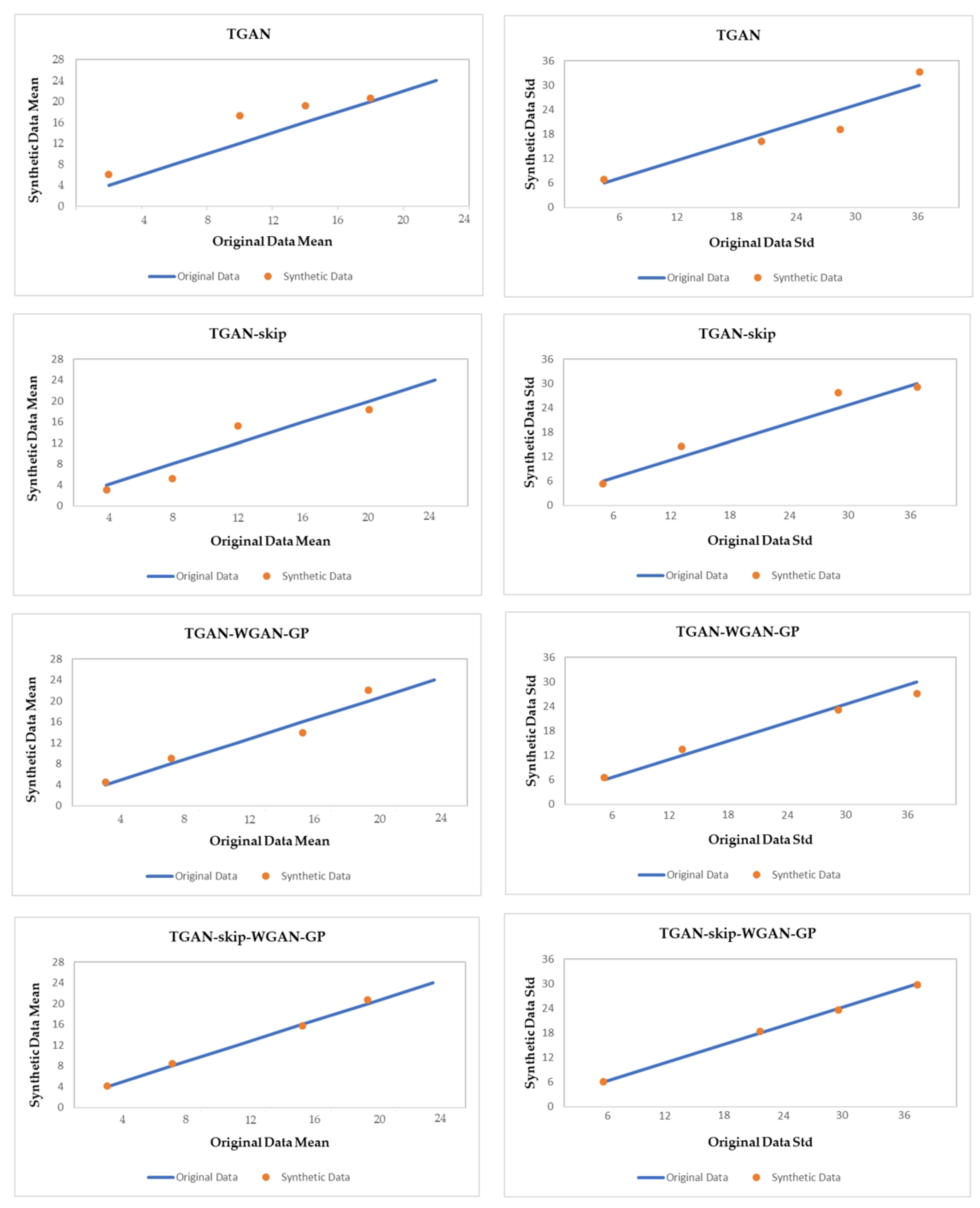
For visual evaluation, we plotted the mean and standard deviation of each column. The plotted values that are closer to the diagonal have better mean and deviation. The closer the values of each column get to the diagonal, the more correlated they are. We compare the mean and standard deviation result of TGAN, TGAN-skip, TGAN–WGAN-GP, and our proposed method TGAN-skip–WGAN-GP for the synthetic data in Figure 10. As results show, the mean and standard deviation of each column using TGAN-skip–WGAN-GP are closest to the diagonal and produce better results than other GAN models.

3.2.7. Cumulative Sum

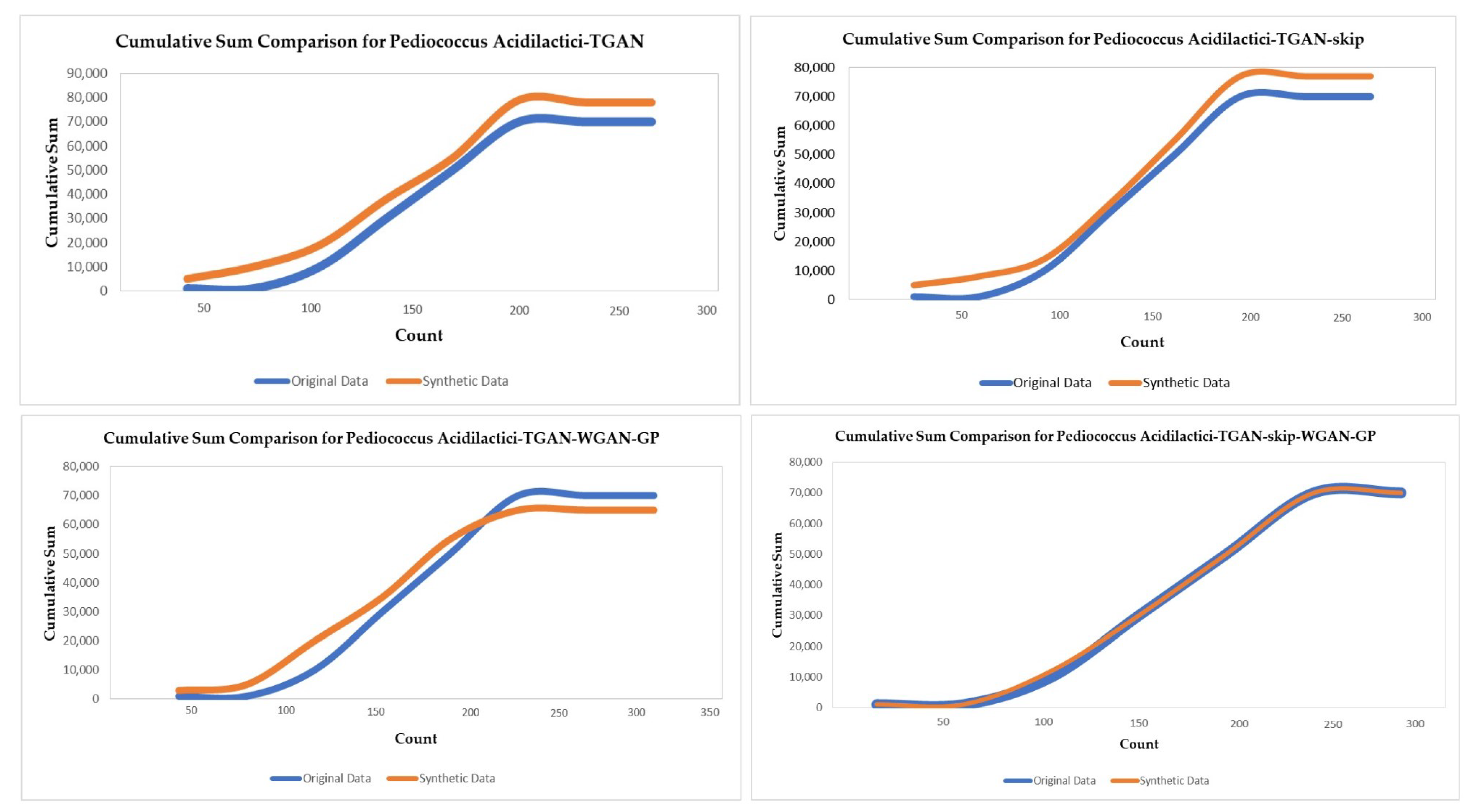
Cumulative sum displays the distribution per column for original and generated synthetic data in Figure 11. In the figure, we show the count distribution of Pediococcus acidilactici for original and generated synthetic data for four different models of GAN. Cumulative sum can be used to evaluate both continuous and categorical values. We can see from Figure 11 that the distribution of Pediococcus acidilactici using TGAN-skip–WGAN-GP is the most closely related.

3.2.8. Maximum Mean Discrepancy

The maximum mean discrepancy (MMD) is a measure for distance between two distributions in a reproducing kernel Hilbert space on the mean embeddings. The measured MMD values for our original and synthetic samples were 0.6 and 0.3, respectively, which evaluated our synthetic data to be better.

4. Conclusions

In this paper, we proposed a methodology to successfully generate synthetic tabular data for Shindari fermentation, using multiple imputation ensemble and generative adversarial networks. We first preprocessed the data and used multivariate imputation by chained equations and random forest imputation to fill the missing data. For prediction, we used ensemble methods called bagging and stacking. We tested our model with different regressors, among which random forest produced the best result with low values for Kappa error plots. In the Results section, we produced experimentation results for different combinations of the imputation and ensemble methods, which show that our proposed methodologies MICE-Bag, MICE-SE, RFI-Bag, and RFI-SE produce low error rates and obtain higher accuracy with low mean dissimilarity. A visual presentation of the original and imputed data for every microbial community has also been provided in this paper.
After multiple imputation ensemble, we perform data transformation, which provides more meaning to the data. For generating synthetic data, we proposed TGAN-skip–WGAN-GP, which is an architectural combination of TGAN-skip and WGAN-GP. We added skip connections to the normal TGAN model and inherited the architecture of WGAN-GP into TGAN, which resulted in better performance, eliminated the mode collapse problem, and reduced the convergence time. After synthesizing, we performed inverse transformation, and finally, we obtained the tabular synthetic data for Shindari fermentation. We evaluated the quality of synthetic data based on correlation coefficient, MAE, RMSE, PRD, FD, and mirror column association. Mean and standard deviation were shown in the paper for different GAN models on our dataset. Cumulative sum visually represented the distribution of data per column, showing that TGAN-skip–WGAN-GP performs significantly better for generating synthetic tabular data than existing GAN models.

Author Contributions

Conceptualization, D.H.; formal analysis, D.H.; funding acquisition, Y.-C.B.; methodology, D.H.; writing—review and editing, D.H.; investigation, Y.-C.B.; resources, Y.-C.B.; project administration, Y.-C.B.; supervision, Y.-C.B. All authors have read and agreed to the published version of the manuscript.

Funding

This research was financially supported by the Ministry of Small and Medium-sized Enterprises(SMEs) and Startups(MSS), Korea, under the “Regional Specialized Industry Development Program(R&D, S2855401)” supervised by the Korea Institute for Advancement of Technology(KIAT).

Institutional Review Board Statement

Not applicable

Informed Consent Statement

Informed consent was obtained from all subjects involved in the study.

Acknowledgments

We would like to thank Chang-Gu Hyun and Minseo Byun for collaborating with us and providing us the dataset.

Conflicts of Interest

The authors declare no conflict of interest regarding the design of this study, analyses, and writing of this manuscript.

References

  1. Hyun, S.B.; Hyun, C.G. Anti-Inflammatory Effects and Their Correlation with Microbial Community of Shindari, a Traditional Jeju Beverage. Fermentation 2020, 6, 87. [Google Scholar] [CrossRef]
  2. Leroy, F.; De Vuyst, L. Lactic acid bacteria as functional starter cultures for the food fermentation industry. Trends Food Sci. Technol. 2004, 15, 67–78. [Google Scholar] [CrossRef]
  3. Fagan, R.P.; McLaughlin, J.B.; Castrodale, L.J.; Gessner, B.D.; Jenkerson, S.A.; Funk, E.A.; Hennessy, T.W.; Middaugh, J.P.; Butler, J.C. Endemic foodborne botulism among Alaska Native persons—Alaska, 1947–2007. Clin. Infect. Dis. 2011, 52, 585–592. [Google Scholar] [CrossRef] [Green Version]
  4. Hartmann, K.G.; Schirrmeister, R.T.; Ball, T. EEG-GAN: Generative adversarial networks for electroencephalograhic (EEG) brain signals. arXiv 2018, arXiv:1806.01875. [Google Scholar]
  5. Oord, A.v.d.; Dieleman, S.; Zen, H.; Simonyan, K.; Vinyals, O.; Graves, A.; Kalchbrenner, N.; Senior, A.; Kavukcuoglu, K. Wavenet: A generative model for raw audio. arXiv 2016, arXiv:1609.03499. [Google Scholar]
  6. Golany, T.; Radinsky, K.; Freedman, D. SimGANs: Simulator-Based Generative Adversarial Networks for ECG Synthesis to Improve Deep ECG Classification. In Proceedings of the International Conference on Machine Learning, Vienna, Austria, 12–18 July 2020; pp. 3597–3606. [Google Scholar]
  7. Kearney, V.; Chan, J.W.; Wang, T.; Perry, A.; Descovich, M.; Morin, O.; Yom, S.S.; Solberg, T.D. DoseGAN: A generative adversarial network for synthetic dose prediction using attention-gated discrimination and generation. Sci. Rep. 2020, 10, 1–8. [Google Scholar] [CrossRef]
  8. De Chazal, P.; O’Dwyer, M.; Reilly, R.B. Automatic classification of heartbeats using ECG morphology and heartbeat interval features. IEEE Trans. Biomed. Eng. 2004, 51, 1196–1206. [Google Scholar] [CrossRef] [Green Version]
  9. Eduardo, A.; Aidos, H.; Fred, A. ECG-based biometrics using a deep autoencoder for feature learning-an empirical study on transferability. In Proceedings of the International Conference on Pattern Recognition Applications and Methods, Porto, Portugal, 24–26 February 2017; Volume 2, pp. 463–470. [Google Scholar]
  10. Bishop, C.M. Pattern Recognition and Machine Learning; Springer: Berlin/Heisenberg, Germany, 2006. [Google Scholar]
  11. Rajpurkar, P.; Hannun, A.Y.; Haghpanahi, M.; Bourn, C.; Ng, A.Y. Cardiologist-level arrhythmia detection with convolutional neural networks. arXiv 2017, arXiv:1707.01836. [Google Scholar]
  12. Güler, I.; Übeyli, E.D. Adaptive neuro-fuzzy inference system for classification of EEG signals using wavelet coefficients. J. Neurosci. Methods 2005, 148, 113–121. [Google Scholar] [CrossRef] [PubMed]
  13. Prasad, G.K.; Sahambi, J. Classification of ECG arrhythmias using multi-resolution analysis and neural networks. In Proceedings of the TENCON 2003, Conference on Convergent Technologies for Asia-Pacific Region, Bangalore, India, 15–17 October 2003; Volume 1, pp. 227–231. [Google Scholar]
  14. Kachuee, M.; Fazeli, S.; Sarrafzadeh, M. Ecg heartbeat classification: A deep transferable representation. In Proceedings of the 2018 IEEE International Conference on Healthcare Informatics (ICHI), New York, NY, USA, 4–7 June 2018; pp. 443–444. [Google Scholar]
  15. Al Rahhal, M.M.; Bazi, Y.; AlHichri, H.; Alajlan, N.; Melgani, F.; Yager, R.R. Deep learning approach for active classification of electrocardiogram signals. Inf. Sci. 2016, 345, 340–354. [Google Scholar] [CrossRef]
  16. Choi, E.; Biswal, S.; Malin, B.; Duke, J.; Stewart, W.F.; Sun, J. Generating multi-label discrete patient records using generative adversarial networks. arXiv 2017, arXiv:1703.06490. [Google Scholar]
  17. Torfi, A.; Beyki, M. Generating Synthetic Healthcare Records Using Convolutional Generative Adversarial Networks; Virginia Tech: Blacksburg, VA, USA, 2019. [Google Scholar]
  18. Jordon, J.; Yoon, J.; van der Schaar, M. PATE-GAN: Generating synthetic data with differential privacy guarantees. In Proceedings of the International Conference on Learning Representations, Vancouver, BC, Canada, 30 April–3 May 2018. [Google Scholar]
  19. Narváez, P.; Percybrooks, W.S. Synthesis of Normal Heart Sounds Using Generative Adversarial Networks and Empirical Wavelet Transform. Appl. Sci. 2020, 10, 7003. [Google Scholar] [CrossRef]
  20. Aznan, N.K.N.; Atapour-Abarghouei, A.; Bonner, S.; Connolly, J.D.; Al Moubayed, N.; Breckon, T.P. Simulating brain signals: Creating synthetic eeg data via neural-based generative models for improved ssvep classification. In Proceedings of the 2019 International Joint Conference on Neural Networks (IJCNN), Budapest, Hungary, 14–19 July 2019; pp. 1–8. [Google Scholar]
  21. Hernandez-Matamoros, A.; Fujita, H.; Perez-Meana, H. A novel approach to create synthetic biomedical signals using BiRNN. Inf. Sci. 2020, 541, 218–241. [Google Scholar] [CrossRef]
  22. Aleryani, A.; Wang, W.; De La Iglesia, B. Multiple Imputation Ensembles (MIE) for dealing with missing data. SN Comput. Sci. 2020, 1, 1–20. [Google Scholar] [CrossRef] [Green Version]
  23. Buuren, S.V.; Groothuis-Oudshoorn, K. Mice: Multivariate imputation by chained equations in R. J. Stat. Softw. 2010, 45, 1–68. [Google Scholar] [CrossRef] [Green Version]
  24. Tang, F.; Ishwaran, H. Random forest missing data algorithms. Stat. Anal. Data Mining Asa Data Sci. J. 2017, 10, 363–377. [Google Scholar] [CrossRef] [PubMed]
  25. Tukey, J.W. Exploratory Data Analysis; Reading; Addison-Wesley: Boston, MA, USA, 1977; Volume 2. [Google Scholar]
  26. Ensemble Methods: Bagging, Boosting and Stacking. Available online: https://towardsdatascience.com/ensemble-methods-bagging-boosting-and-stacking-c9214a10a205 (accessed on 10 January 2020).
  27. Goodfellow, I.; Pouget-Abadie, J.; Mirza, M.; Xu, B.; Warde-Farley, D.; Ozair, S.; Courville, A.; Bengio, Y. Generative adversarial nets. Adv. Neural Inf. Process. Syst. 2014, 27, 2672–2680. [Google Scholar]
  28. Brenninkmeijer, B.; de Vries, A.; Marchiori, E.; Hille, Y. On the Generation and Evaluation of Tabular Data Using GANs. Master’s Thesis, Radboud University, Nijmegen, The Netherlands, 2019. [Google Scholar]
  29. Xu, L.; Veeramachaneni, K. Synthesizing tabular data using generative adversarial networks. arXiv 2018, arXiv:1811.11264. [Google Scholar]
  30. Arjovsky, M.; Chintala, S.; Bottou, L. Wasserstein gan. arXiv 2017, arXiv:1701.07875. [Google Scholar]
  31. Gulrajani, I.; Ahmed, F.; Arjovsky, M.; Dumoulin, V.; Courville, A.C. Improved training of wasserstein gans. In Proceedings of the 31st International Conference on Neural Information Processing Systems, Long Beach, CA, USA, 4–9 December 2017; pp. 5767–5777. [Google Scholar]
  32. Khan, S.S.; Ahmad, A.; Mihailidis, A. Bootstrapping and multiple imputation ensemble approaches for classification problems. J. Intell. Fuzzy Syst. 2019, 37, 7769–7783. [Google Scholar] [CrossRef]
  33. Hazra, D.; Byun, Y.C. SynSigGAN: Generative Adversarial Networks for Synthetic Biomedical Signal Generation. Biology 2020, 9, 441. [Google Scholar] [CrossRef] [PubMed]
  34. Zhu, F.; Ye, F.; Fu, Y.; Liu, Q.; Shen, B. Electrocardiogram generation with a bidirectional LSTM-CNN generative adversarial network. Sci. Rep. 2019, 9, 1–11. [Google Scholar] [CrossRef] [PubMed] [Green Version]
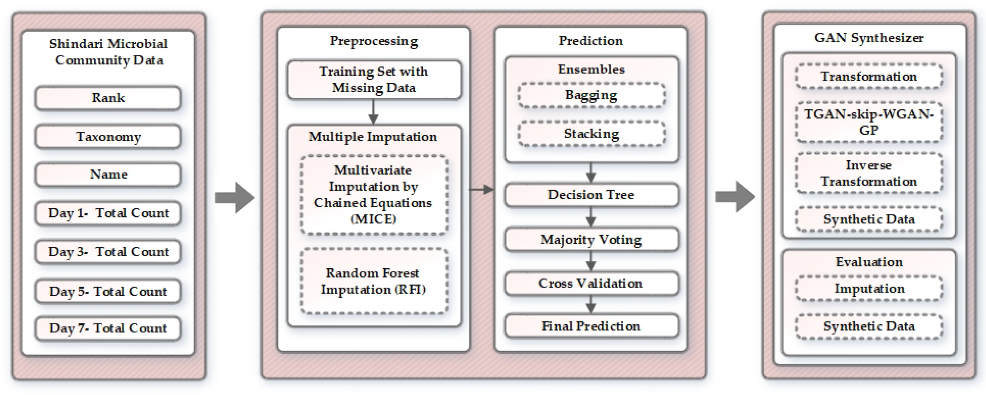
Figure 1. Overview of the proposed approach.
Applsci 11 02787 g001
Figure 2. Layout of Shindari microbial community data.
Applsci 11 02787 g002
Figure 3. Architecture of Bagging Ensemble.
Applsci 11 02787 g003
Figure 4. Architecture of Stacking Ensemble.
Applsci 11 02787 g004
Figure 5. Overview of the generative adversarial network.
Applsci 11 02787 g005
Figure 6. Layout of TGAN-skip–WGAN-GP: (a) Layout of TGAN-skip architecture. (b) Architecture of the generator. (c) Architecture of the discriminator. TGAN—Temporal generative adversarial network; WGAN—Wasserstein GAN; GP—gradient penalty.
Applsci 11 02787 g006
Figure 7. Original count of the microbial community.
Applsci 11 02787 g007
Figure 8. Imputed distribution of the microbial community.
Applsci 11 02787 g008
Figure 9. Results of the imputation, generating count for each microbial community every 6 h.
Applsci 11 02787 g009
Figure 10. Mean and standard deviation comparison of different GAN models in our data.
Applsci 11 02787 g010
Figure 11. Cumulative sum of coloum ‘count’ for the Pediococcus acidilactici microbial community.
Applsci 11 02787 g011
Table 1. Mean dissimilarity, regressor accuracy and Kappa error plots for different imputation methods. SV—support vector; DT—decision tree; RF—random forest; SL—simple linear; Bag—bagging ensemble; SE—stacking ensemble.
Regressor Accuracy
Imputation
Method
Mean
Dissimilarity
SVDTRFSLKappa
Error Plots
GRI-Bag0.9165.5478.1279.1873.410.785
GRI-SE0.9367.5676.1379.2972.840.712
EMB-Bag0.8668.9880.2982.5175.820.854
EMB-SE0.8270.1281.6682.7877.150.844
RFI-Bag0.4678.7782.8795.0371.670.513
RFI-SE0.4371.3485.6794.3771.020.490
MICE-Bag0.5171.9188.4291.1278.440.566
MICE-SE0.5675.2388.9993.9776.350.519
Table 2. Definition of correlation values.
Correlation ValuesDepiction
0 to 0.3 or 0 to −0.3Negligibly correlated
0.3 to 0.5 or −0.3 to −0.5Low correlation
0.5 to 0.7 or −0.5 to −0.7Moderately correlated
0.7 to 0.9 or −0.7 to −0.9Highly correlated
0.9 to 1 or −0.9 to 1Extensively correlated
Table 3. Performance comparison of various GAN models with our proposed TGAN-skip–WGAN-GP model.
ModelMean
Correlation
Coefficient
MAERMSEPRDFDMirror
Column
Association
TGAN0.6730.770.5988.210.870.629
TGAN-skip0.8150.650.6271.350.890.714
TGAN–WGAN-GP0.9370.560.5861.730.710.863
TGAN-skip–WGAN-GP0.9810.410.3651.820.680.947
Publisher’s Note: MDPI stays neutral with regard to jurisdictional claims in published maps and institutional affiliations.