Abstract
This paper puts forward a 1-D convolutional neural network (CNN) that exploits a novel analysis of the correlation between the two leads of the noisy electrocardiogram (ECG) to classify heartbeats. The proposed method is one-dimensional, enabling complex structures while maintaining a reasonable computational complexity. It is based on the combination of elementary handcrafted time domain features, frequency domain features through spectrograms and the use of autoregressive modeling. On the MIT-BIH database, a 95.52% overall accuracy is obtained by classifying 15 types, whereas a 95.70% overall accuracy is reached when classifying 7 types from the INCART database.
1. Introduction and Related Work
Cardiovascular diseases are the first cause of death in the world, with an estimated 17.9 million deaths each year. Among them, heart arrhythmia qualifies as an abnormal heart rhythm that can result in serious complications such as stroke or cardiac deaths. Early detection of arrhythmia is a major challenge for our society.
With electrocardiograms (ECGs), heartbeats can be visually labelled according to several classes such as Normal beat, Supraventricular escape beat, etc. An ECG is a graph of voltage versus time of the electrical activity of the heart using electrodes placed on the skin. To assess the condition of the heart from different angles, an ECG has several leads, each of them being the signal generated by a pair of electrodes.
In the last decades, researchers employed machine learning methods for the automatic classification of heartbeats contained in long-duration recordings of human ECGs [1,2]. A traditional heartbeat classification pipeline includes data preprocessing, data segmentation, feature extraction, feature selection, and classification [3].
Data preprocessing is used to remove noise from the ECG raw signal. The most used techniques are median filters [4], discrete wavelet transform (DWT) [5,6], adaptive filters [4,7], and frequency selective filters [8,9,10].
Data segmentation is used to isolate heartbeats from the whole ECG recording. Once a time segment including the heartbeat is available, time domain [11,12,13,14,15,16] or frequency domain [13,16,17,18] or morphological [11,12,13,15,16] or statistical [13,19] or neural features [20] are extracted.
Feature selection is used to reduce the number of features used by the classifier thus reducing the complexity and time required for computation. Several approaches have been adopted: principal and independent component analysis [5,6,21,22], linear discriminant analysis [6], and genetic algorithm [23].
Random forest [24,25], support vector machines (SVMs) [13,14,15,16,18,19], neural networks (NNs) [5,6] or deep neural networks (DNNs) [2,26,27,28,29,30,31,32] are employed to classify extracted features in one of the heartbeat classes.
As discussed above, ECGs can be recorded in different locations of the body thus obtaining the so-called multilead ECGs. Up to 12 leads can be recorded and each lead represents a specific characteristic of the heart. Multilead ECGs better reflect the state of the heart compared with single lead ECGs. Taking into account multi leads may bring performance improvement. Existing literature is mainly focused on the processing of single lead ECGs [20].
In this paper, we focus on two-lead ECGs: we use lead V1, that is a chest lead, and lead II, that is a limb lead. We propose the combination of hand-crafted features with a canonical correlation analysis network (CCANet) and SVMs for two-lead heartbeats classification. The analysis of the correlation between two leads of the ECG is exploited to increase heartbeat classification performance [20]. Proposed CCANet is a 1-D variant of the original 2-D CCANet proposed by Yang et al. [20] that allows to explore a deeper CCANet while maintaining a reasonable computational complexity and providing better results. CCANet has been originally proposed by Yang et al. [33] for the processing of two-view images in 2017. Compared to one-view image-based PCANet and RandNet, CCANet demonstrated to perform better [33]. CCANet has also been employed in other computer vision tasks such as remote sensing scene classification [34] as well as ECG interpretation [20].
There are two types of CNNs that are commonly used for ECG classification: the 1-D CNN and 2-D CNN [35]. 2-D CNNs usually operate on transformed ECG data, such as spectrograms, gray-level co-occurrence matrices, combined features and others. 1-D CNNs operate directly on the raw ECG signal. Our one-dimensional variant takes as input a combination of elementary hand crafted time domain features, frequency domain features through spectrograms, and the use of autoregressive modeling.
For the sake of comparison, we evaluate a suitable implemented 1-D convolutional neural network (CNN) solution based on residual networks (ResNet) [36]. ResNet demonstrated to be one of the most performing CNN for visual recognition [37]. The proposed method outperforms the state of the art on both the MIT-BIH and INCART arrhythmia databases.
Our Contribution
The main novel contributions of this paper are summarized as follows:
- We have designed a novel one-dimensional canonical correlation analysis network (1-D CCANet) to exploit two-lead ECGs for automatic classification of heartbeats that outperforms the state of the art;
- We have explored the use of handcrafted features in combination with a 1-D CCANet for ECG classification;
- Our proposal outperforms a solution based on a suitable one-dimensional ResNet that we have implemented for the sake of comparison.
2. Materials
2.1. MIT-BIH Database
The MIT-BIH database contains 48 sets of two-lead ECG signals (lead II and mostly V1). Each signal is approximately 30 min long, has been collected at a 360 Hz sampling frequency, and has been independently annotated by at least two cardiologists. Annotations include the 15 types listed in Table 1. In our study, we use the signals for which both II and V1 leads are available (see PhysioBank for further details).

Table 1.
Details of the categories for MIT-BIH database.
2.2. INCART Database
The St. Petersburg Institute of Cardiological Techniques 12-lead arrhythmia database (INCART) contains 75 sets of 12-lead ECG signals (leads I, II, III, aVR, aVL, aVF, V1, V2, V3, V4, V5, V6). Each signal is approximately 30 min long and has been collected at a 257 Hz sampling frequency. We only consider leads II and V1 of each record. Annotations include the 7 types listed in Table 2.
Table 2.
Details of the categories for INCART database.
3. Proposed Method
The input of the proposed method is a two-channel ECG segment obtained after a preliminary segmentation that consists in the isolation of heartbeats in each record. Given the R-peak positions, any heartbeat is isolated by retaining and samples to the left and to the right of the R-peak, respectively. For each of the two leads, a vector denoted as is built with the values of the ECG (in Volts), of size . The values of and are 160–200 and 120–136 for MIT-BIH and INCART, respectively. These values are given in Table 3, and are similar to the one used in [20].
Table 3.
Sampling rates, values of and for both MIT-BIH and INCART databases.
The architecture of the whole process is shown Figure 1a,b. The first stage is feature extraction. The input of the process is, for each lead, a vector (with ) containing raw values of the segmented heartbeat. Each lead is normalized (see the “Normalization” module in Figure 1a by using a rescaling procedure so that the resulting vector has an intensity that ranges from 0 to 1, as per equation:
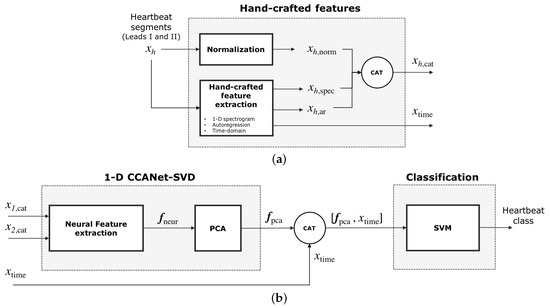
Figure 1.
Classification processing pipeline of our method. (a) Feature extraction: for each of the two leads , hand-crafted features are extracted to build while , a vector of time-domain features, is built for both leads. (b) Part of these features, , feeds the 1-D CCANet-SVD module, which first outputs the neural features and then a reduced version of the neural features . The concatenation of and feeds the classification module. The output is the predicted heartbeat class.
At the same time, hand-crafted features are extracted from each lead : frequency-domain features , and autoregression features . A single time-domain features vector is also computed for both leads. Frequency-domain features, autoregression features and the normalized segmented heartbeat are concatenated to obtain the vector (see Figure 1a). The vector is processed by the neural module to produce a single output vector for the two leads (see Figure 1b). The vector is then reduced in dimensions by using Principal Component Analysis (PCA) thus obtaining the vector . The concatenation of the time-domain features and is the input of a Support Vector Machine classifier. The output of the classifier is the predicted heartbeat class. In the following subsections the feature extraction and neural module are discussed more in detail.
3.1. Hand-Crafted Feature Extraction
Given an isolated heartbeat , hand-crafted features are extracted with three different methods: frequency-domain, time-domain, autoregressive modeling.
3.1.1. One-Dimensional Spectrogram
For the frequency domain, we use a one-dimensional spectrogram, which is a representation of the spectrum of frequencies of a signal as it varies with time. It is built through a short-time Fourier transform (STFT) of each of the two non-normalized leads . A window slides through the signal (with potential overlapping) and computes at each step the squared magnitudes of the STFT of the portion of the signal belonging to the window. The Hamming windowing is used for this process. The spectrogram is then obtained by concatenating, along the time axis, the squared magnitudes acquired for each window. The squared magnitudes obtained for each frequency (up to half of the sampling rate) at each time step can be reported in a matrix where axis 0 and 1 are the frequency and time axis, respectively. Since the range of the squared magnitudes varies significantly, the resulting matrix is rescaled to to yield .
A weighted average along the frequency axis is performed thus turning the matrix into a one-dimensional vector, . The equation used is the following (2):
where .
This feature extraction method requires three parameters: the number of samples in the window of the STFT ( = 64 and 46 for MIT-BIH and INCART respectively), the number of samples in the overlap between two consecutive steps (= 32 and 23 for MIT-BIH and INCART respectively) and n (0.25 for both MIT-BIH and INCART), the weight parameter in Equation (2). Suitable parameters are found with a greedy search. The feature vector is of size 10.
3.1.2. Autoregressive Modeling
Autoregressive (AR) modeling specifies that a time series value depends linearly on its own previous values and a stochastic term, as per Equation (3):
where is the time series, are the AR coefficients computed with Yule-Walker’s method and p is the order of the AR model. Since the choice of the order p depends highly on the sampling rate, non-normalized ECGs from both databases are resampled to 360 Hz [38]. The order was then chosen by performing best parameter search on the training data for both the MIT-BIH and INCART databases. We chose the order that maximized the average of our performance metrics (accuracy, specificity, sensitivity, ppv) on a validation set. Figure 2 shows that for the INCART data, the best order is 2 while the best order is 3 for the MIT-BIH data. Since the performance for MIT-BIH is quite comparable for orders 2 and 3, we chose an order equal to 2 for both datasets. We preferred a lower order to reduce the computational cost. The vector of AR coefficients obtained for each lead of one heartbeat, , is denoted as and is of size 2.
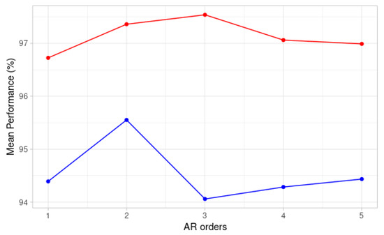
Figure 2.
Mean performance for different AR orders on validation sets for MIT-BIH signals (red) and INCART signals (blue).
3.1.3. Time-Domain Features
For each of the two leads of one segmented heartbeat, we compute the following time-domain features: the median value of , its fourth order and fifth order central moments and the kurtosis of . Finally, for both leads, we build a single vector of time-domain features including the previous features for each lead and the heartbeat rate of the patient to whom the heartbeat belongs. The resulting vector is denoted as and is of size 9.
3.2. Neural Feature Extraction
To exploit the correlation between two ECG leads, we use a one-dimensional variant of the canonical correlation analysis network (CCANet). First introduced in the field of image recognition by Yang et al. [33], CCANet has been employed in two-view image recognition tasks. Recently, CCANets, which are intrinsically two-dimensional, have been successfully employed in the signal processing field for the classification of two and three lead heartbeats [20]. A CCANet is usually composed of two cascaded convolutional layers and an output layer: (1) in the convolutional layers, the CCA technique is used to extract dual-lead filter banks; (2) in the output layer, the features extracted from the second convolutional layer are mapped into the final feature vector [20].
In this paper, with the aim of increasing performance, we design a new 1-D canonical correlation analysis network that is composed of four 1-D convolutional layers and an output layer. Contrary to CCANet, the filters are found by combining a CCA with a singular value decomposition (SVD), and features are extracted after each layer. The use of 1-D convolutions instead of 2-D permits to limit computational cost, thus allowing to increase the number of layers from two to four and, consequently, to increase performance.
The processing pipeline is shown in Figure 3. The input of the proposed 1-D CCANet-SVD is the concatenation of autoregressive features, spectrogram features, and the original normalized heartbeat, resulting in the following vector , . The 1-D CCANet-SVD is trained with N two-lead heartbeats and then used as neural feature extractor in combination with a linear SVM for heartbeat classification. The network is trained separately for the MIT-BIH and INCART databases.
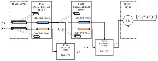
Figure 3.
Proposed 1-D CCANet-SVD.
3.2.1. First Convolutional Layer
We denote the i-th element () of an input vector . We selected a series of segments of size k centered on each value , to obtain the m following segments, . The latter are then zero-centered and concatenated to build a matrix of the segments . This procedure is performed on each of the N training heartbeats and the resulting matrices of segments are finally concatenated to obtain , . Note that our network is simultaneously fed with all the training heartbeats in order to build the two matrices and .
Let us address the filter extraction stage. In [20], the filters are found with a CCA, thus by maximizing the correlation between pairs of projected variables. The first projection direction can be obtained by optimizing Equation (4):
with the constraints , where , and and are the first canonical vectors for each of the two leads. The Lagrange multiplier technique shows that and are eigenvectors of and , respectively. Given the first directions, the l-th projection direction can be calculated by solving problem (4) with the additional constraints , . In the end, the filters for the first lead are built by taking the primary eigenvectors of (i.e. associated with the biggest eigenvalues), whereas the filters for the second lead are built by considering the primary eigenvectors of .
In this paper, we use a slightly different approach, referred to as the CCA-SVD filter extraction technique. We perform an SVD of both , and , as per and , where the U and V matrices are unitary, and the D matrices are diagonal with singular values on the diagonals. Using an SVD allows to retrieve the directions, which explain the most the variance of and . Since these two matrices derive from the CCA, they capture the correlations between the two leads. Therefore, we use the directions found by performing an SVD on them to have the best explanation of the correlation between the two leads. Consequently, the filters for the first lead are built by taking the columns of that are associated with the biggest singular values of , whereas the filters for the second lead are built by considering the columns of that are associated with the biggest singular values of . Such an approach yields better results than the traditional CCA filter extraction technique (see Experiments). We denote as and , , the filters of size k corresponding to the first and second lead, respectively.
As for the convolutions, for each lead h, each input signal yields outputs , . The length of the input and output signal were kept identical, thanks to a zero-padding of the input.
3.2.2. First Extraction Stage
The extraction stage follows the same steps as in [20]. First, for each heartbeat, the output of the first convolution is converted to a decimal one-dimensional signal as per , where H is the Heaviside step function. Therefore, the range of each component of T is . T is then divided in B blocks of size . Each block can overlap with its neighbor, according to , an overlapping proportion parameter. For each of these blocks, a histogram with bins is built. The values of the resulting histogram for each block is embedded in a -long vector and the vectors provided by each block are then concatenated to obtain . The first feature vector, for the heartbeat, is .
3.2.3. Second Convolution Layer and Extraction Stage
The second layer is identical to the previous one, except for the fact that the input is different. Indeed, before the first convolution, each lead of a heartbeat was represented by a single vector of length m. After the first convolution, each lead is now represented by vectors of length m. Let’s walk through the second layer with the notations used so far.
The , produced after the first convolutional layer are the input of the second layer. Since we initially considered N training heartbeats, it means that this layer has a total number of input vectors corresponding to lead 1 and input vectors corresponding to lead 2. The same segmentation and zero-centering process as in the first layer gives , the matrices of the concatenated segments for all the input vectors, for each lead.
Applying the CCA-SVD filter extraction technique with leads us to perform the SVD of and , for the first and second lead, respectively. The filters are then found exactly as in the first convolutional layer and we denote as and , , the filters of size k extracted for the first and second lead, respectively.
As for the convolutions, for each initial lead and channel , the signal yields outputs , . At this stage, each initial lead of a heartbeat is now represented by vectors of size m.
The second extraction step is the same as after the first convolutional layer except for a few points. First, for each heartbeat, the output of the second convolutional layer is converted to a decimal signal as per , . The second feature vector for the heartbeat is obtained as per . The are built with a block size and an overlapping parameter equal to and , respectively.
The third and fourth convolutional layers are built similarly. and refer to the third and fourth feature vectors extracted for a heartbeat after each layer. We denote as and , the number of filters for the third and fourth layers, respectively. and are the block sizes for the construction of after the third and fourth convolutional layers, respectively. Finally, we denote as and , the overlapping parameters for the last two layers.
3.2.4. Final Output and PCA
For a given heartbeat, the final output of the network is obtained by concatenating the four feature vectors, as per . Given the significant size of the final feature vector, a PCA is carried out to reduce dimensionality. The number of components is chosen such that the explained variance is over 99.99% thus obtaining . The final feature vector is obtained by concatenating this vector to the vector of time-domain features corresponding to the heartbeat. is a vector of size 1382 or 3020, for INCART or MIT-BIH heartbeats, respectively.
The classification step is performed by a linear SVM, with a regularization parameter .
4. Experiments
4.1. Experimental Setup
To assess the performance of our method, we classified 15 and 7 different types of heartbeats from the MIT-BIH and INCART databases, respectively. One major obstacle of our databases is that they are not well balanced. For instance, the normal types are over-represented while the supraventricular escape beats from INCART have few samples in comparison. To address this issue, we randomly sampled (without repetition), as in [20], 3350 heartbeats from the MIT-BIH database and 1720 heartbeats from INCART, in the proportions given by Table 1 and Table 2 respectively.
We used k-fold cross validation on the resampled heartbeats to fit the parameters of 1-D CCANet-SVD. The parameters are shown in Table 4.
Table 4.
Parameters for 1-D CCANet-SVD.
The results provided in the Results and discussion subsection derive from an overall confusion matrix obtained after summing the k confusion matrices given after each fold. As in [20], we performed 10 and 5-cross validation for the data from the MIT-BIH and INCART databases, respectively.
The code is written in Python 3.7 and we ran all the experiments on a personal computer equipped with Ubuntu 18.04. The hardware specifications of the computer are the following: 16 GB RAM, and i7-7700 CPU with a clock speed of 3.60 GHz.
1-D ResNet
To further validate our approach, we added a one-dimensional residual network (1-D ResNet) to our experiments. The input is the same as for 1-D CCANet-SVD. The 1-D ResNet has been implemented as follows:
- Initial layer: the input of the network undergoes an initial convolution with 2 input channels (one for each lead) and 16 output channels. This convolution is followed by a max-pooling step. This initial layer is followed by 4 identical residual blocks.
- Residual blocks: each of them contains two convolutional layers and, for each block, the output of the second convolutional layer is finally added to the block’s input. For each block, the first convolution doubles the number of channels, while the second convolution has the same number of input and output channels. Consequently, the last convolution has 256 output channels. The output of the last block then undergoes average-pooling to obtain the feature vector.
- Classification layer: the feature vector, of size 256 serves as the input of a fully connected neural network. The classification is then performed thanks to the Softmax function. The loss used is the cross-entropy.
During the feature extraction process, Batch-Normalization is performed after each convolution and the Rectified Linear Unit (ReLU) is used as the activation function. Table 5 shows the architecture of the network and the various parameters fitted for each layer. All the parameters, including the number of layers, residual blocks and the number of channels for the convolutions were found through cross-validation.
Table 5.
Architecture of 1-D ResNet with the parameters for the initial layer and the convolutions of each residual block.
4.2. Evaluation Metrics
Several measures have been employed for the evaluation of the goodness of the proposed approach: (1) Overall Accuracy (OACC) defined as (TP + TN)/(TP + TN + FP + FN); (2) Mean Accuracy (MACC) defined as the average of the class accuracies; (3) Specificity (SPE) defined as TN/(TN + FP); (4) Sensitivity (SENS) defined as TP/(TP + FN); (5) Positive Predictive Values (PPV) defined as TP/(TP + FP). TP, TN, FP, FN are the number of True Positive, True Negative, False Positive and False Negative, respectively. Note that in Table 6, the values of SPE, SENS, and PPV are averaged across the classes.
Table 6.
Results for various methods (%). For each method, first line reports results for the MIT-BIH database while the second line reports for the INCART database. OACC stands for Overall Accuracy; MACC for Mean Accuracy; SPE for Specificity; SENS for Sensitivity; PPV for Positive Predictive Values; AVG is the Average of the first 5 columns of the table. Best results are highlighted in boldface.
4.3. Results and Discussion
Table 6 shows the results obtained for various classification methods. It includes the previously described model, variations of it (e.g., without adding the time-domain features), the 1-D ResNet and the best dual-leads method in the state of the art [20].
Our method and [20] demonstrated comparable performances on the MIT-BIH database, though our overall accuracy and mean ppv were better by around 0.3%. As for the INCART database, our results proved to be better, especially the overall accuracy (+1.69%), mean sensitivity (+2.89%), and mean ppv (+1.78%). Contrary to [20], our approach is purely one-dimensional, allowing to explore a more complex version of CCANet while maintaining a reasonable computational complexity and providing better results: we opted for 4 layers and stacking features extracted after each convolution gave better results than without doing so (see seventh method of Table 6), especially increasing the sensitivity. Using frequency features with the one-dimensional spectrogram helped obtain a better classification by notably increasing the sensitivity (+1.12% for INCART) and the ppv (+1.3% for INCART). The addition of the AR coefficients and the time-domain features contributed to slightly increase the performance of our model. The performances were significantly better when using our CCA-SVD filter extraction technique instead of the CCA technique described in [20], with a sensitivity gaining more than for INCART (see the third method of Table 6). Finally, our method provided significantly better results than the 1-D ResNet approach (+3.64% for overall ACC for MIT-BIH, +9.45% for INCART). Our analysis of the correlations of the two leads, using SVD, proved to be a good way of recognizing the various types of heartbeats.
Table 7 and Table 8 show the comparison between the best of our proposals and similar works in the state of the art for MIT-BIH and INCART databases respectively. In the case of MIT-BIH, Table 7 confirms that the use of dual-leads-based approaches brings improvements in performance (more than 1%). Also in the case of INCART we see an improvement with respect to single-lead-based method (more than 3%). Here, the proposed approach is slightly better than a variant of the work by Yang et al. [20] that uses three leads. Although our approach explores more complex structures with respect to Yang et al. [20], it remains comparable, in terms of computational cost, with it. The inference time for each heart beat classification is about 0.05 s while in the case of Yang et al. [20], it is about 0.02 s.
Table 7.
Results for various methods on the MIT-BIH database.
Table 8.
Results for various methods on the INCART database.
Our method presents a few limitations. First, the CCANet technique requires the network to be fed simultaneously with all the training data, in order to determine the filters and this may cause a growth in the computational cost as the size of the training data increases. This limitation is common to all the CCANet-based architectures. In our study, we only considered 2-lead signals as input, it could be interesting to include more leads with the hope of increasing the performance, especially for classes with fewer samples. Following the work by Yang et al. [20], our approach can be quite naturally extended to 3-lead signals. The number of layers might need to be reduced to compensate for the additional cost added by the addition of a third lead. Another interesting perspective would be to include some of the techniques we have used in our study in the original two-dimensional CCANet developed by Yang et al. [20]. Indeed, Table 6 shows that the use of the SVD significantly increases the performance, without adding additional computational cost compared to the original method. Therefore, we could also expect promising results when using SVD in the original 2-D CCANet. Likewise, it could be interesting to analyze how the spectrogram features influence the performance of the 2-D CCANet and allow to make significant improvement in the field of abnormal heartbeat recognition.
5. Conclusions
In this paper, we propose a novel heartbeat classification method based mainly on a new approach to the study of the correlation between the two ECG leads, to extract complex features. Our method also employ elementary hand-crafted time domain features, frequency domain features with a one-dimensional approach to spectrograms, and autoregressive coefficients. Our method is one-dimensional, allowing to explore a more complex neural architecture while maintaining a reasonable computational complexity, and providing better results. Our final model has an optimal structure and performs the classification of 15 and 7 heartbeat types for the MIT-BIH and INCART databases, respectively. Finally, our method outperforms [20] with a slightly better overall accuracy and mean ppv on the MIT-BIH database and a notably higher overall accuracy (+1.69%), mean sensitivity (+2.89%), and mean ppv (+1.78%) on the INCART database.
Author Contributions
All the authors contributed equally to the conceptualization; all the authors contributed equally to the methodology; all the authors contributed equally to the software; all the authors contributed equally to the validation; all the authors contributed equally to the draft preparation; all the authors contributed equally to the writing, review and editing. All authors have read and agreed to the published version of the manuscript.
Funding
This research received no external funding.
Institutional Review Board Statement
Not applicable.
Informed Consent Statement
Not applicable.
Data Availability Statement
Not applicable.
Conflicts of Interest
The authors declare no conflict of interest.
References
- Rim, B.; Sung, N.J.; Min, S.; Hong, M. Deep Learning in Physiological Signal Data: A Survey. Sensors 2020, 20, 969. [Google Scholar] [CrossRef] [PubMed]
- Hannun, A.Y.; Rajpurkar, P.; Haghpanahi, M.; Tison, G.H.; Bourn, C.; Turakhia, M.P.; Ng, A.Y. Cardiologist-level arrhythmia detection and classification in ambulatory electrocardiograms using a deep neural network. Nat. Med. 2019, 25, 65. [Google Scholar] [CrossRef] [PubMed]
- Bhirud, B.; Pachghare, V. Arrhythmia detection using ECG signal: A survey. In Proceeding of the International Conference on Computational Science and Applications, Pune, India, 7–9 August 2019; pp. 329–341. [Google Scholar]
- Mathews, S.M.; Kambhamettu, C.; Barner, K.E. A novel application of deep learning for single-lead ECG classification. Comput. Biol. Med. 2018, 99, 53–62. [Google Scholar] [CrossRef]
- Elhaj, F.A.; Salim, N.; Harris, A.R.; Swee, T.T.; Ahmed, T. Arrhythmia recognition and classification using combined linear and nonlinear features of ECG signals. Comput. Methods Programs Biomed. 2016, 127, 52–63. [Google Scholar] [CrossRef] [PubMed]
- Martis, R.J.; Acharya, U.R.; Min, L.C. ECG beat classification using PCA, LDA, ICA and discrete wavelet transform. Biomed. Signal Process. Control 2013, 8, 437–448. [Google Scholar] [CrossRef]
- Venkatesan, C.; Karthigaikumar, P.; Paul, A.; Satheeskumaran, S.; Kumar, R. ECG signal preprocessing and SVM classifier-based abnormality detection in remote healthcare applications. IEEE Access 2018, 6, 9767–9773. [Google Scholar] [CrossRef]
- Alonso-Atienza, F.; Morgado, E.; Fernandez-Martinez, L.; García-Alberola, A.; Rojo-Alvarez, J.L. Detection of life-threatening arrhythmias using feature selection and support vector machines. IEEE Trans. Biomed. Eng. 2013, 61, 832–840. [Google Scholar] [CrossRef]
- Xia, Y.; Zhang, H.; Xu, L.; Gao, Z.; Zhang, H.; Liu, H.; Li, S. An automatic cardiac arrhythmia classification system with wearable electrocardiogram. IEEE Access 2018, 6, 16529–16538. [Google Scholar] [CrossRef]
- Hammad, M.; Maher, A.; Wang, K.; Jiang, F.; Amrani, M. Detection of abnormal heart conditions based on characteristics of ECG signals. Measurement 2018, 125, 634–644. [Google Scholar] [CrossRef]
- Soria, M.L.; Martínez, J. Analysis of multidomain features for ECG classification. In Proceedings of the 2009 36th Annual Computers in Cardiology Conference (CinC), Park City, UT, USA, 13–16 September 2009; pp. 561–564. [Google Scholar]
- De Lannoy, G.; François, D.; Delbeke, J.; Verleysen, M. Weighted conditional random fields for supervised interpatient heartbeat classification. IEEE Trans. Biomed. Eng. 2011, 59, 241–247. [Google Scholar] [CrossRef]
- Pławiak, P. Novel methodology of cardiac health recognition based on ECG signals and evolutionary-neural system. Expert Syst. Appl. 2018, 92, 334–349. [Google Scholar] [CrossRef]
- Huang, H.; Liu, J.; Zhu, Q.; Wang, R.; Hu, G. A new hierarchical method for inter-patient heartbeat classification using random projections and RR intervals. Biomed. Eng. Online 2014, 13, 90. [Google Scholar] [CrossRef] [PubMed]
- Zhang, Z.; Dong, J.; Luo, X.; Choi, K.S.; Wu, X. Heartbeat classification using disease-specific feature selection. Comput. Biol. Med. 2014, 46, 79–89. [Google Scholar] [CrossRef]
- Zhang, Z.; Luo, X. Heartbeat classification using decision level fusion. Biomed. Eng. Lett. 2014, 4, 388–395. [Google Scholar] [CrossRef]
- Llamedo, M.; Martínez, J.P. Heartbeat classification using feature selection driven by database generalization criteria. IEEE Trans. Biomed. Eng. 2010, 58, 616–625. [Google Scholar] [CrossRef]
- Pławiak, P.; Acharya, U.R. Novel deep genetic ensemble of classifiers for arrhythmia detection using ECG signals. Neural Comput. Appl. 2020, 32, 11137–11161. [Google Scholar] [CrossRef]
- Park, K.; Cho, B.; Lee, D.; Song, S.; Lee, J.; Chee, Y.; Kim, I.Y.; Kim, S. Hierarchical support vector machine based heartbeat classification using higher order statistics and hermite basis function. In Proceedings of the 2008 Computers in Cardiology, Bologna, Italy, 14–17 September 2008; pp. 229–232. [Google Scholar]
- Yang, W.; Si, Y.; Wang, D.; Zhang, G. A novel approach for multi-lead ECG classification using DL-CCANet and TL-CCANet. Sensors 2019, 19, 3214. [Google Scholar] [CrossRef]
- Dohare, A.K.; Kumar, V.; Kumar, R. Detection of myocardial infarction in 12 lead ECG using support vector machine. Appl. Soft Comput. 2018, 64, 138–147. [Google Scholar] [CrossRef]
- Rajagopal, R.; Ranganathan, V. Evaluation of effect of unsupervised dimensionality reduction techniques on automated arrhythmia classification. Biomed. Signal Process. Control 2017, 34, 1–8. [Google Scholar] [CrossRef]
- Li, Q.; Rajagopalan, C.; Clifford, G.D. Ventricular fibrillation and tachycardia classification using a machine learning approach. IEEE Trans. Biomed. Eng. 2013, 61, 1607–1613. [Google Scholar]
- Yang, W.; Si, Y.; Wang, D.; Guo, B. Automatic recognition of arrhythmia based on principal component analysis network and linear support vector machine. Comput. Biol. Med. 2018, 101, 22–32. [Google Scholar] [CrossRef]
- Shimpi, P.; Shah, S.; Shroff, M.; Godbole, A. A machine learning approach for the classification of cardiac arrhythmia. In Proceedings of the 2017 International Conference on Computing Methodologies and Communication (ICCMC), Erode, India, 18–19 July 2017; pp. 603–607. [Google Scholar]
- Park, J.; Kim, J.k.; Jung, S.; Gil, Y.; Choi, J.I.; Son, H.S. ECG-signal multi-classification model based on squeeze-and-excitation residual neural networks. Appl. Sci. 2020, 10, 6495. [Google Scholar] [CrossRef]
- Nurmaini, S.; Umi Partan, R.; Caesarendra, W.; Dewi, T.; Naufal Rahmatullah, M.; Darmawahyuni, A.; Bhayyu, V.; Firdaus, F. An automated ECG beat classification system using deep neural networks with an unsupervised feature extraction technique. Appl. Sci. 2019, 9, 2921. [Google Scholar] [CrossRef]
- Zubair, M.; Kim, J.; Yoon, C. An automated ECG beat classification system using convolutional neural networks. In Proceedings of the 2016 6th International Conference on IT Convergence and Security (ICITCS), Prague, Czech Republic, 26 September 2016; pp. 1–5. [Google Scholar]
- Li, J.; Si, Y.; Lang, L.; Liu, L.; Xu, T. A spatial pyramid pooling-based deep convolutional neural network for the classification of electrocardiogram beats. Appl. Sci. 2018, 8, 1590. [Google Scholar] [CrossRef]
- Acharya, U.R.; Oh, S.L.; Hagiwara, Y.; Tan, J.H.; Adam, M.; Gertych, A.; San Tan, R. A deep convolutional neural network model to classify heartbeats. Comput. Biol. Med. 2017, 89, 389–396. [Google Scholar] [CrossRef]
- Yıldırım, Ö.; Pławiak, P.; Tan, R.S.; Acharya, U.R. Arrhythmia detection using deep convolutional neural network with long duration ECG signals. Comput. Biol. Med. 2018, 102, 411–420. [Google Scholar] [CrossRef]
- Li, H.; Yuan, D.; Ma, X.; Cui, D.; Cao, L. Genetic algorithm for the optimization of features and neural networks in ECG signals classification. Sci. Rep. 2017, 7, 41011. [Google Scholar] [CrossRef]
- Yang, X.; Liu, W.; Tao, D.; Cheng, J. Canonical correlation analysis networks for two-view image recognition. Inf. Sci. 2017, 385, 338–352. [Google Scholar] [CrossRef]
- Yang, X.; Liu, W.; Liu, W. Tensor canonical correlation analysis networks for multi-view remote sensing scene recognition. IEEE Trans. Knowl. Data Eng. 2020. [Google Scholar] [CrossRef]
- Hong, S.; Zhou, Y.; Shang, J.; Xiao, C.; Sun, J. Opportunities and challenges of deep learning methods for electrocardiogram data: A systematic review. Comput. Biol. Med. 2020, 122, 103801. [Google Scholar] [CrossRef]
- He, K.; Zhang, X.; Ren, S.; Sun, J. Deep residual learning for image recognition. In Proceedings of the IEEE Conference on Computer Vision and Pattern Recognition, Las Vegas, NV, USA, 27–30 June 2016; pp. 770–778. [Google Scholar]
- Bianco, S.; Cadene, R.; Celona, L.; Napoletano, P. Benchmark analysis of representative deep neural network architectures. IEEE Access 2018, 6, 64270–64277. [Google Scholar] [CrossRef]
- Ge, D.; Srinivasan, N.; Krishnan, S.M. Cardiac arrhythmia classification using autoregressive modeling. Biomed. Eng. Online 2002, 1, 5. [Google Scholar] [CrossRef] [PubMed]
- Lee, J.N.; Byeon, Y.H.; Pan, S.B.; Kwak, K.C. An EigenECG network approach based on PCANet for personal identification from ECG signal. Sensors 2018, 18, 4024. [Google Scholar] [CrossRef] [PubMed]
Publisher’s Note: MDPI stays neutral with regard to jurisdictional claims in published maps and institutional affiliations. |
© 2021 by the authors. Licensee MDPI, Basel, Switzerland. This article is an open access article distributed under the terms and conditions of the Creative Commons Attribution (CC BY) license (http://creativecommons.org/licenses/by/4.0/).