
Exploiting Data Analytics and Deep Learning Systems to Support Pavement Maintenance Decisions


Abstract
1. Introduction
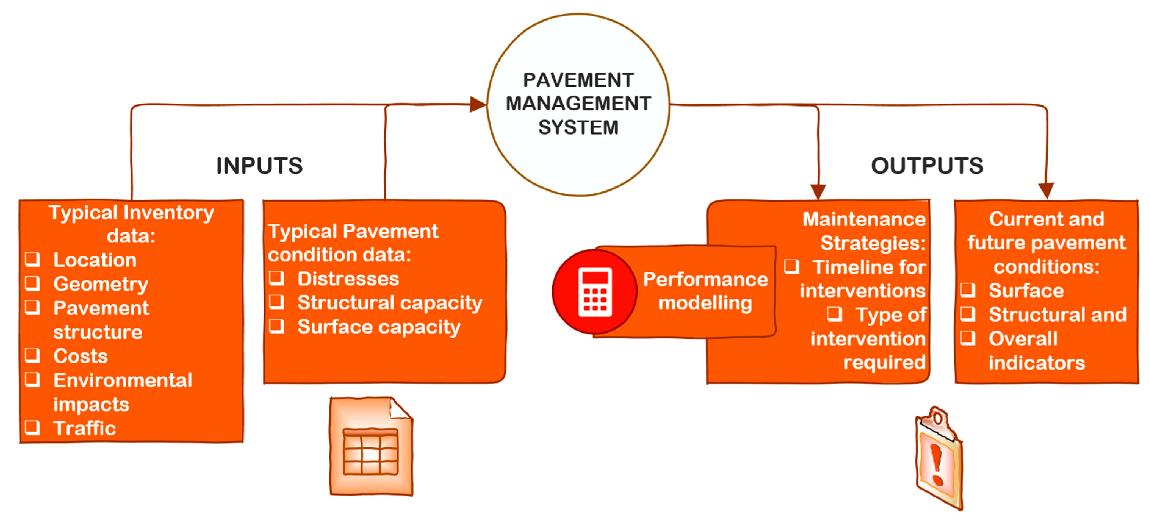
1.1. The Need for Information to Support Pavement Management Decisions
- It serves different types of users within the organization.
- It allows for good decision making concerning the decided programs and projects and allows for the timely execution of projects.
- It makes good use of existing technologies and new ones once they are available.
1.2. Relationship of Factors and Features that Contribute to Pavement Maintenance Interventions
- Network parameters—geometric configuration and dimensions of roads
- Asset values
- Road users—types of users and trip purposes
- Demography and economic circumstances—population and land area
- The density of network and roads
- Use of roads—travel by class
- Safety—accidents and fatalities
1.3. How Have Pavement Management Decisions and Approaches Been Supported by Data Analytics?
1.4. Development of Strategies for Pavement Maintenance in Agencies with Limited Data and Resources
2. Aim of the Study
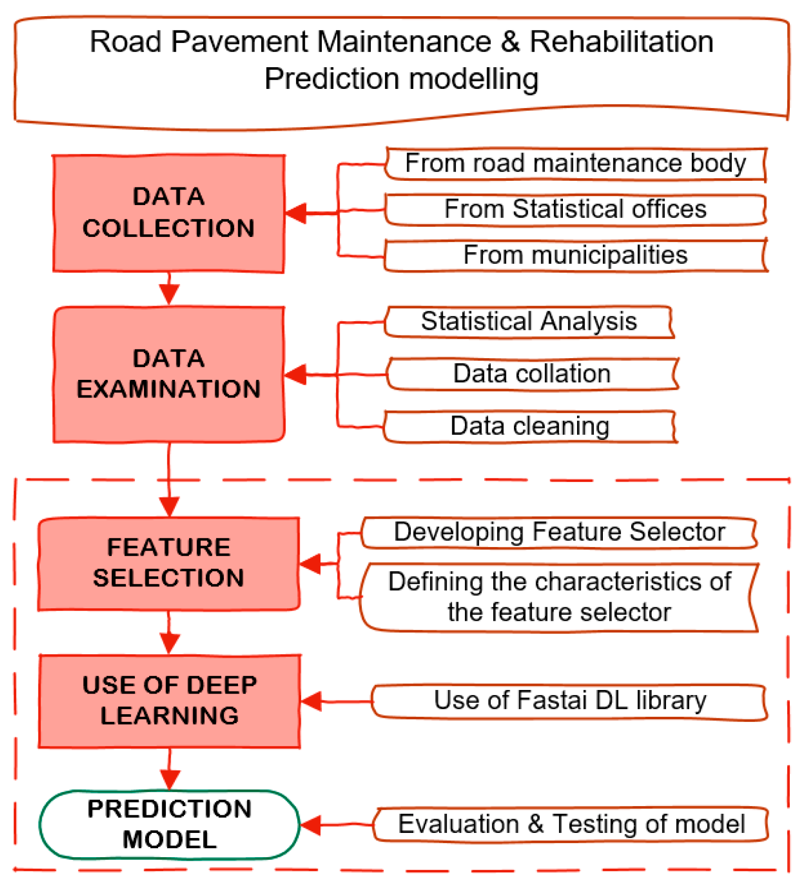
3. Methodology
3.1. Data Collection
3.2. Feature Selection Workflow
3.2.1. Developing Feature Selector
| Algorithm 1: Friedman’s Gradient Boost algorithm |
Inputs:
|
- The library handles categorical features during training as opposed to during the preprocessing time. It also utilizes the entire dataset for training. For each training example, the library carries out a random permutation of the dataset and calculates an average label value for the particular example with the same category value placed before the one provided by the permutation [58].
- The library allows unbiased boosting with categorical features and feature combinations where all the categorical features can be combined as a new feature. [49]
- The use of a fast scorer allows utilizing oblivious trees as base predictors [58].
3.2.2. Defining the Characteristics of the Feature Selector
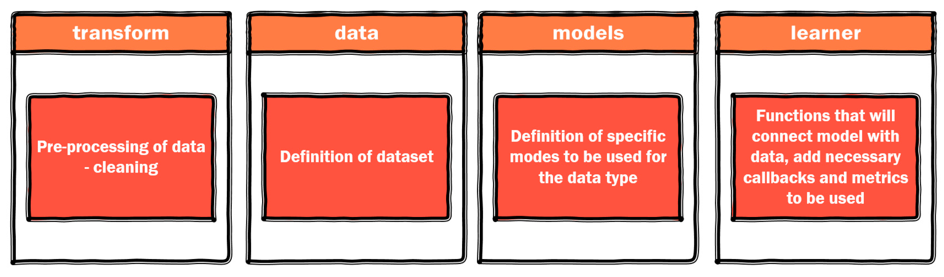
3.3. Use of Deep Learning for Tabular Sets—Use of Fastai Deep Learning Library
3.4. Assessment of the Accuracy of the Model
4. Description of Case Study—Palermo, Italy
Characteristics of Available Data
5. Results and Discussion
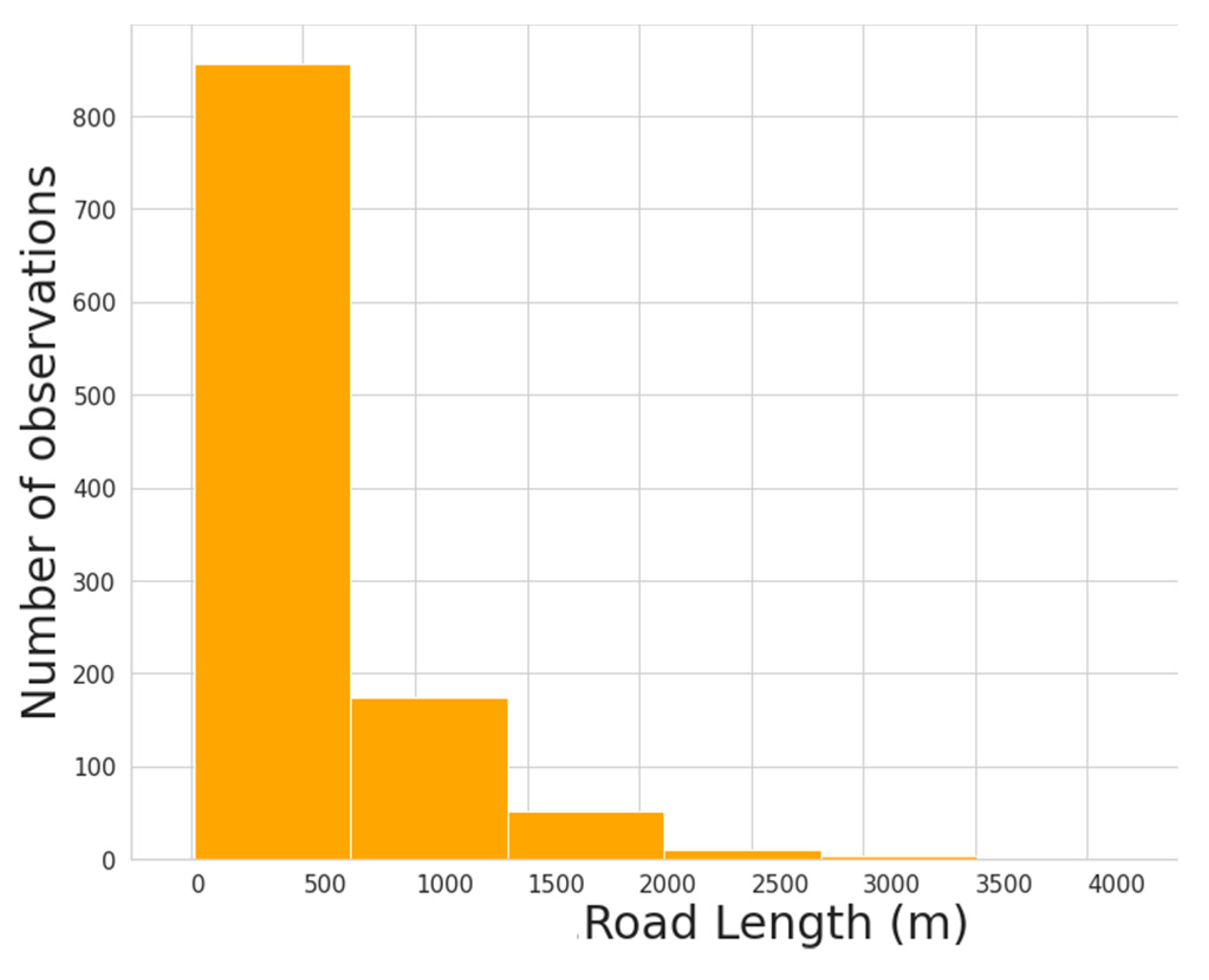
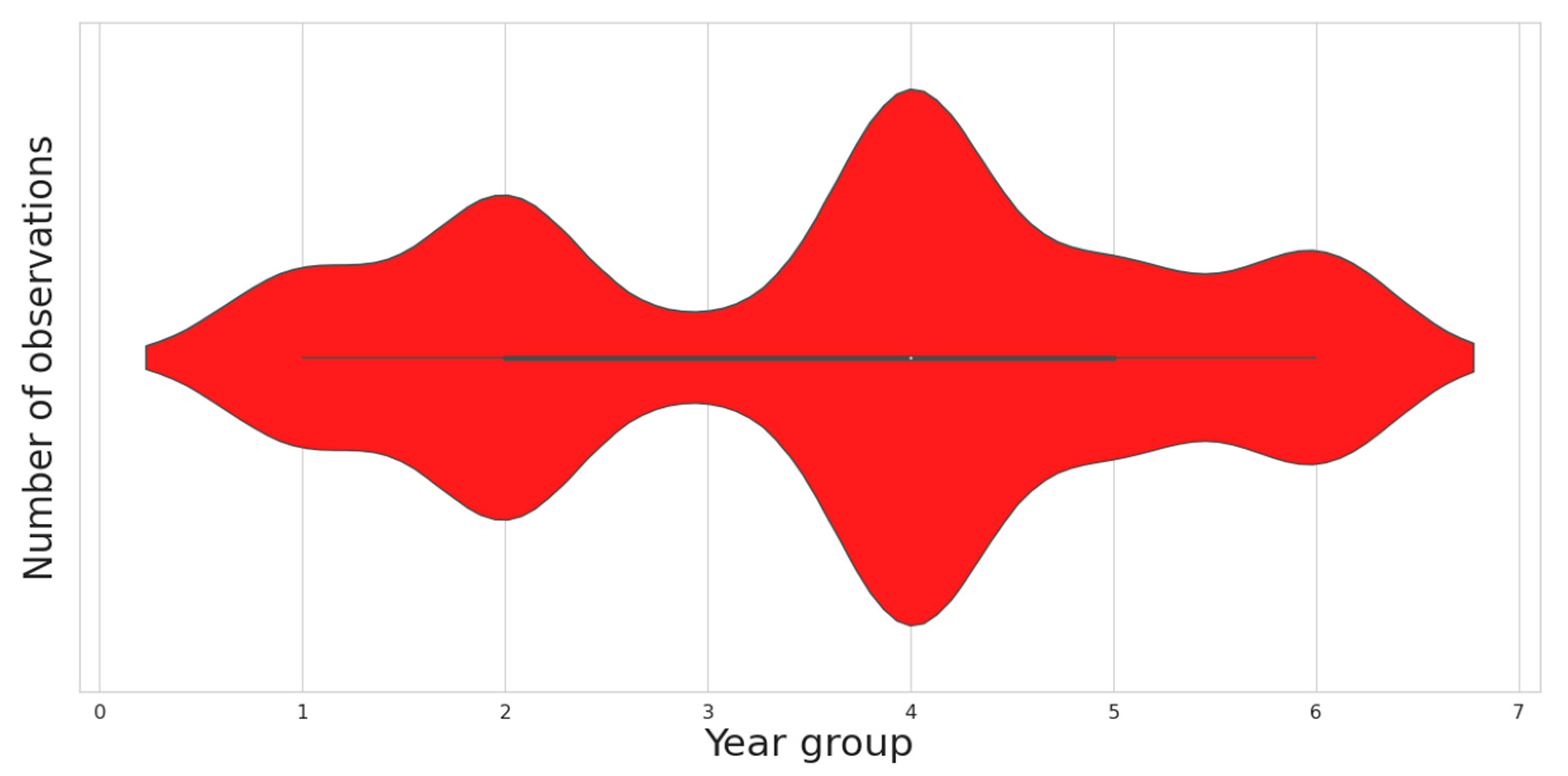
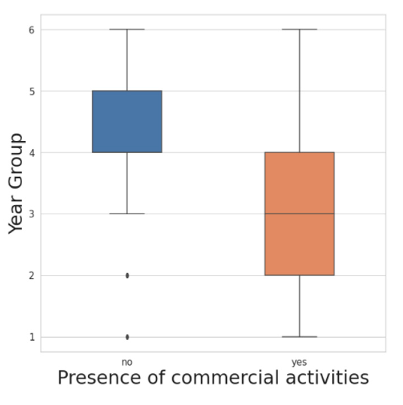
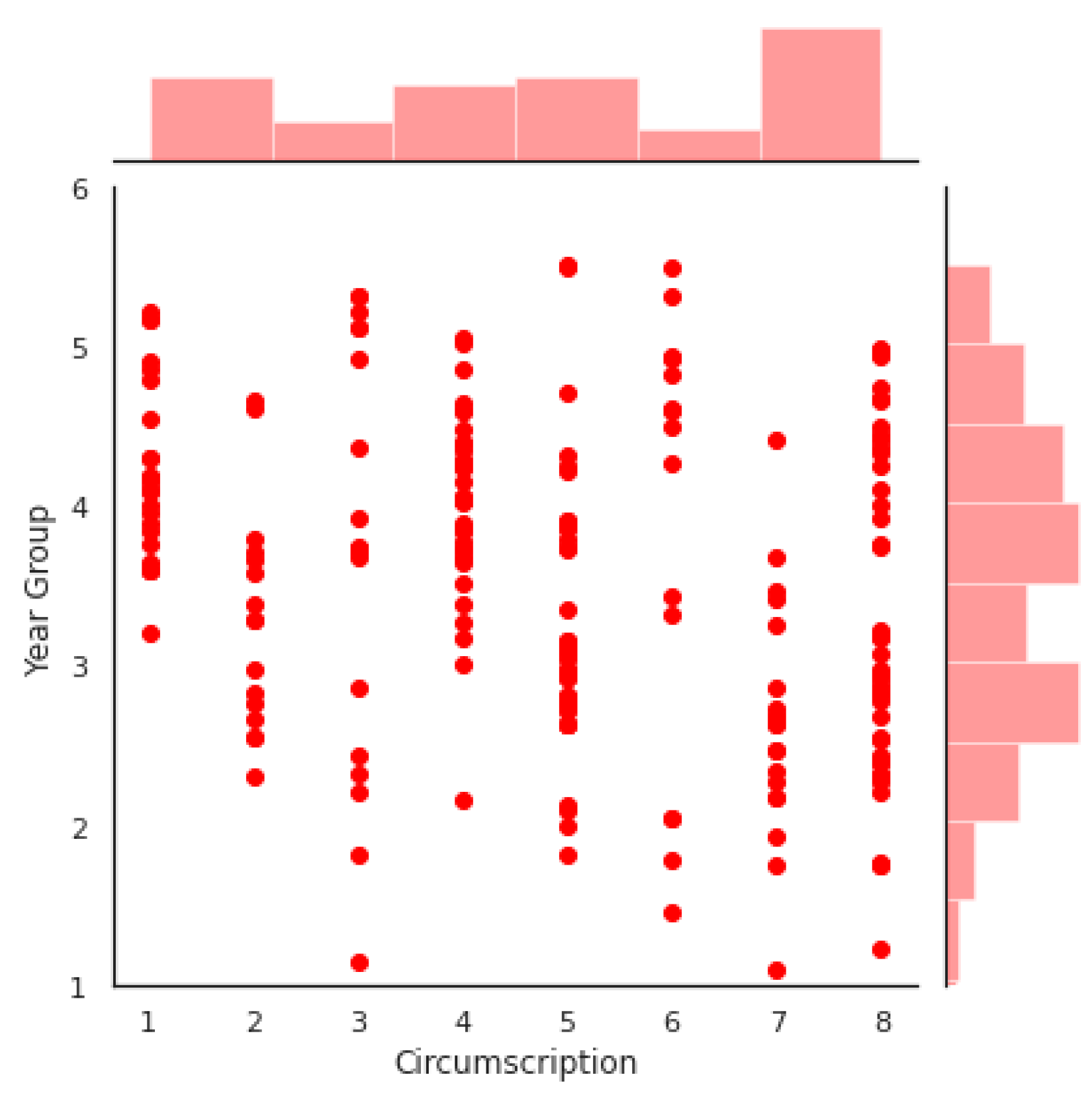
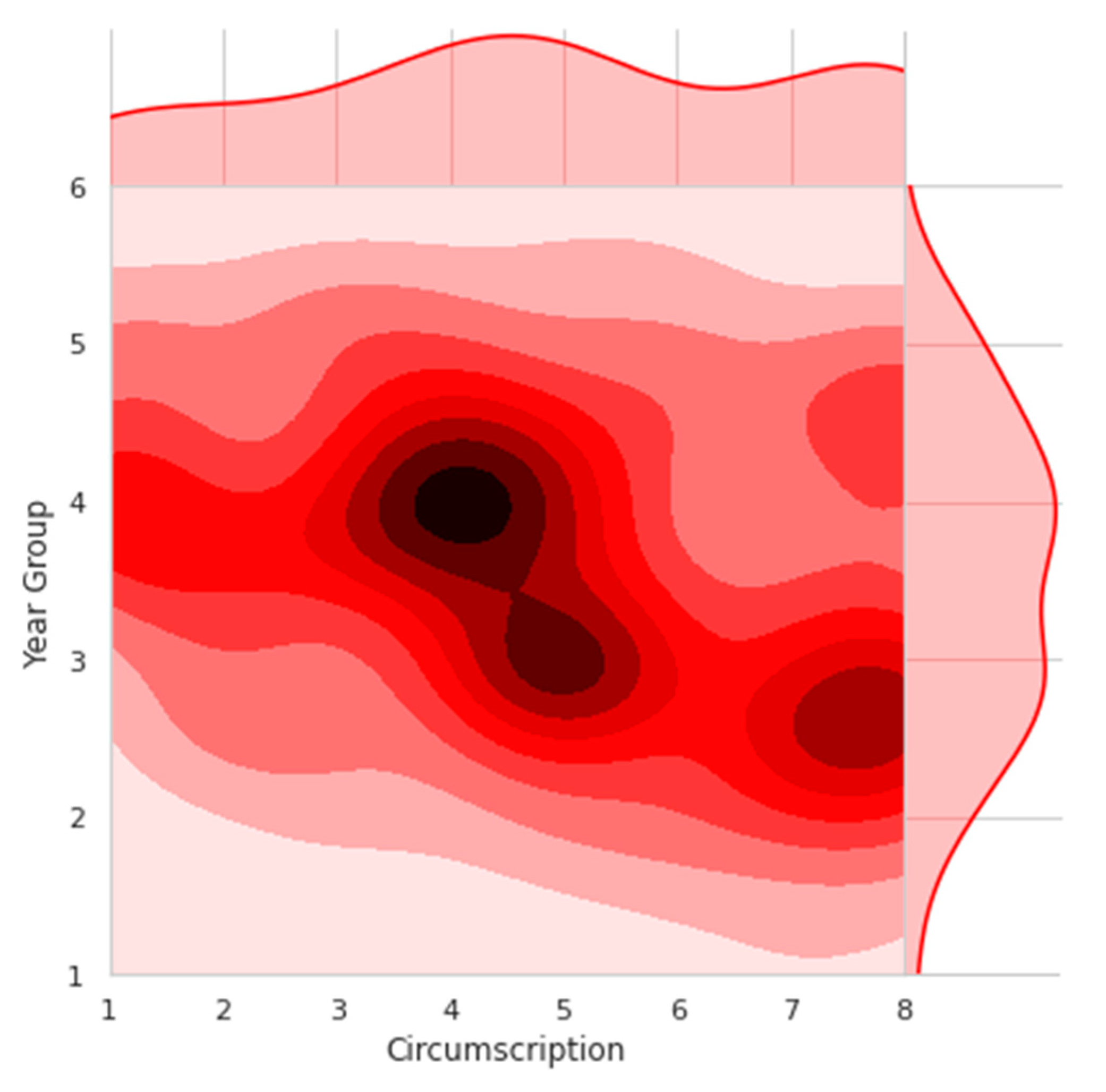
5.1. Examination of Data
5.2. Feature Selection Results
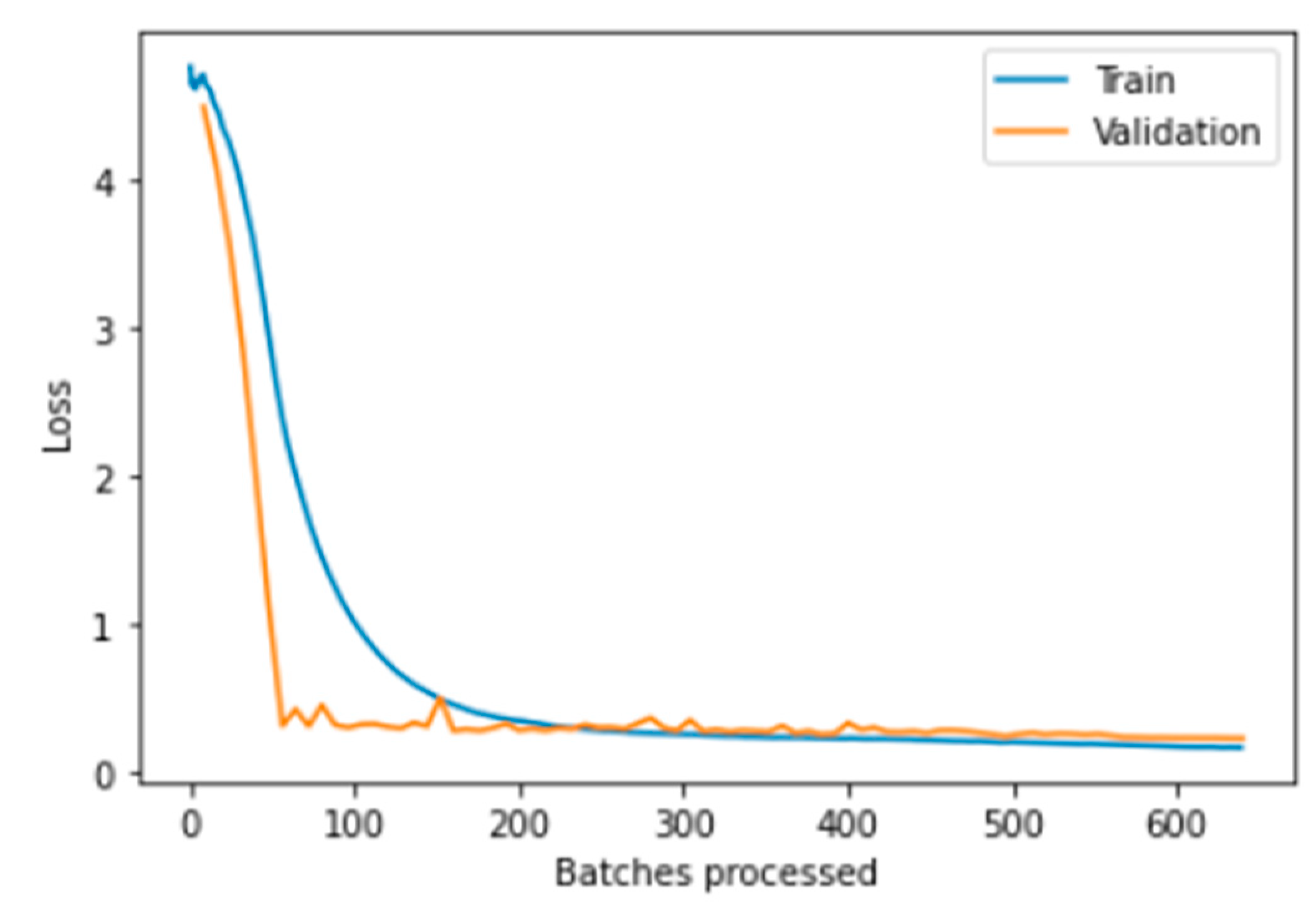
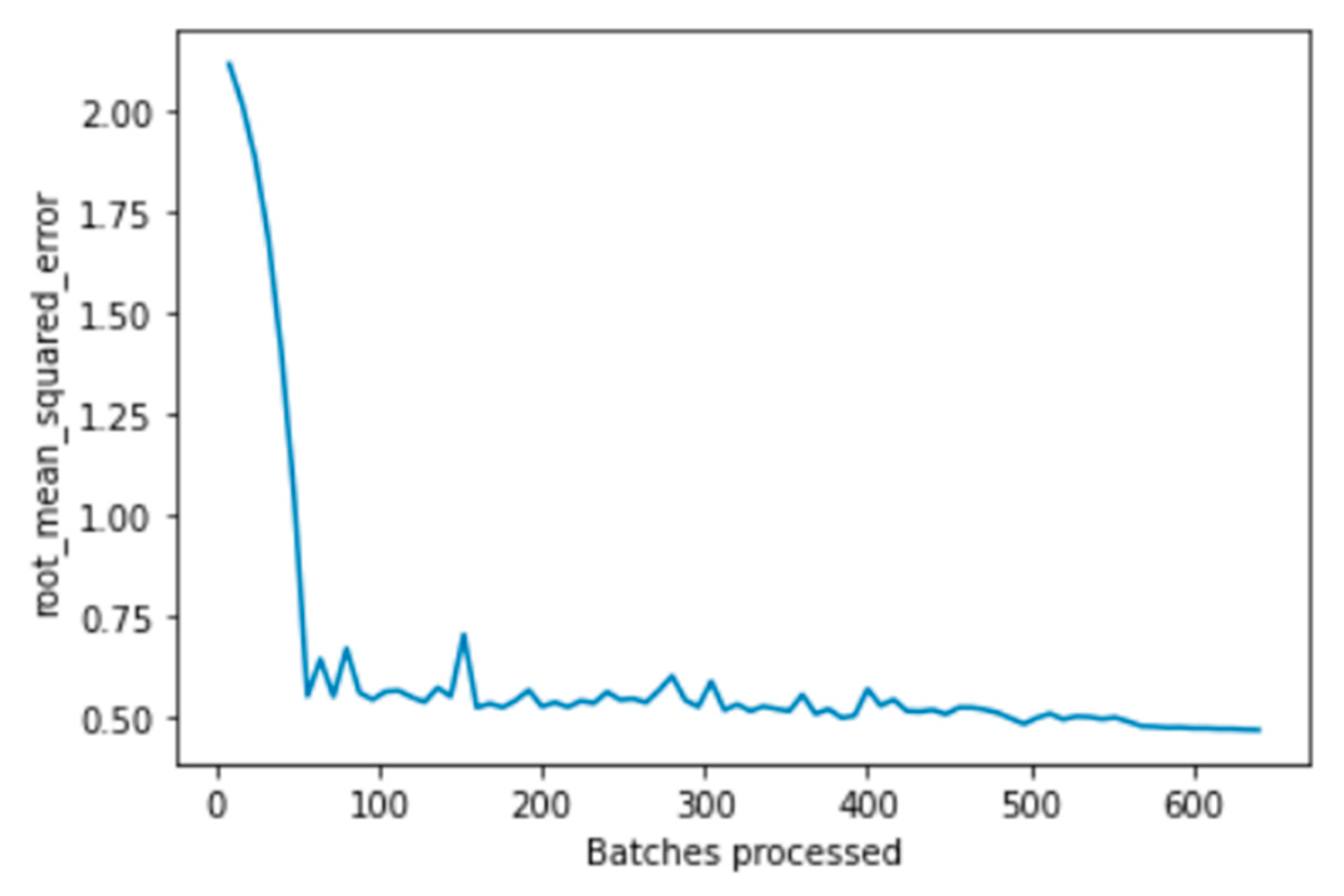
5.3. Fastai Model Results
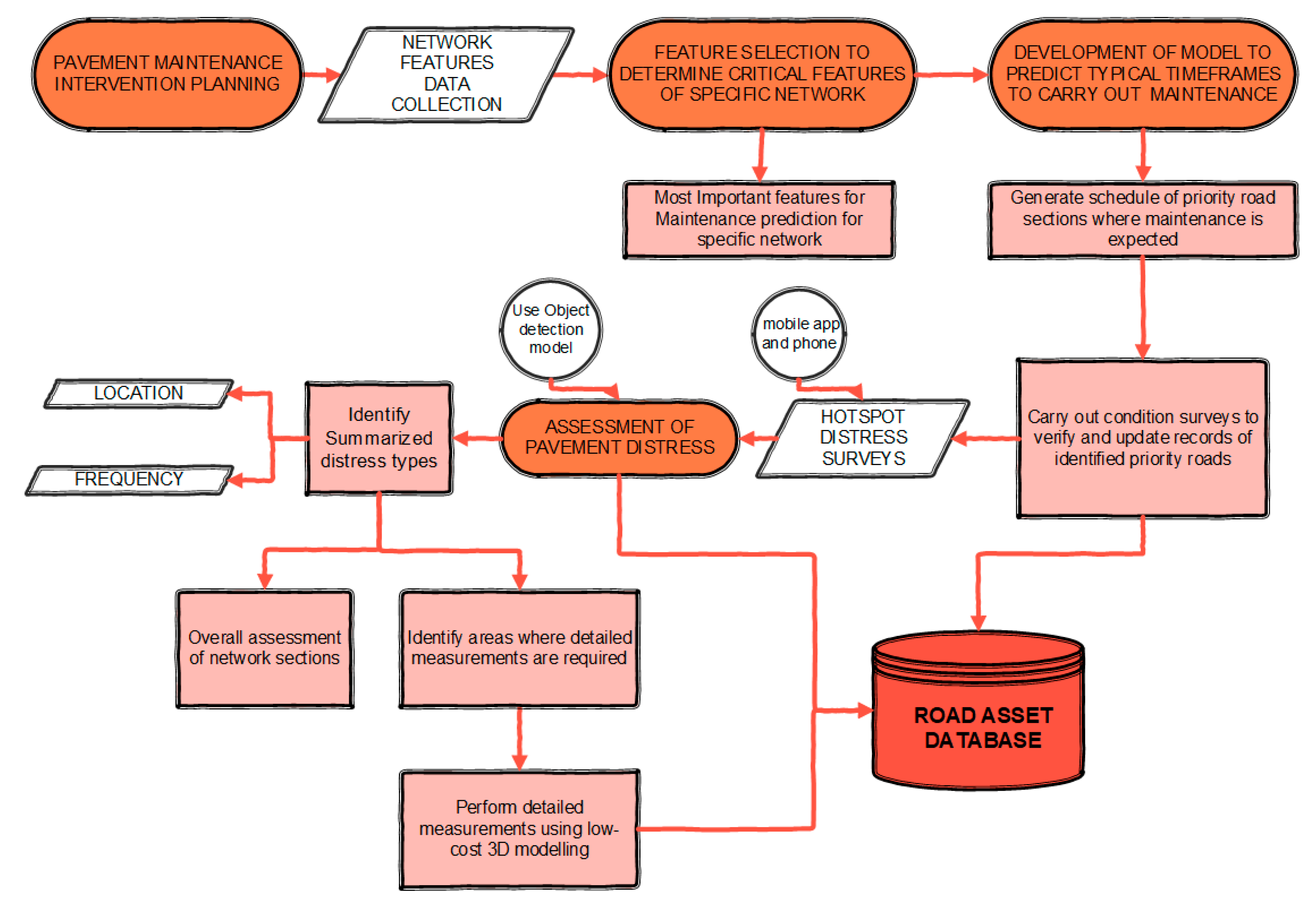
6. Workflow for Practical Implementation with Other Low-Cost Techniques
7. Conclusions
Author Contributions
Funding
Data Availability Statement
Acknowledgments
Conflicts of Interest
Appendix A. Fastai Setup
References
- Vandam, T.J.; Harvey, J.T.; Muench, S.T.; Smith, K.D.; Snyder, M.B.; Al-Qadi, I.L.; Ozer, H.; Meijer, J.; Ram, P.V.; Roesier, J.R.; et al. Towards Sustainable Pavement Systems: A Reference Document FHWA-HIF-15-002; Federal Highway Administration: Washington, DC, USA, 2015. [Google Scholar]
- Eurostat Energy, Transport and Environment Statistics, 2019 ed.; European Union: Brussels, Belgium, 2019; ISBN 9789276109716.
- Karleuša, B.; Dragičević, N.; Deluka-Tibljaš, A. Review of multicriteria-analysis methods application in decision making about transport infrastructure. J. Croat. Assoc. Civ. Eng. 2013, 65, 619–631. [Google Scholar] [CrossRef]
- International Road Federation (IRF). IRF World Road Statistics 2018 (Data 2011–2016); IRF: Brussels, Belgium, 2018. [Google Scholar]
- Mbara, T.C.; Nyarirangwe, M.; Mukwashi, T. Challenges of raising road maintenance funds in developing countries: An analysis of road tolling in Zimbabwe. J. Transp. Supply Chain Manag. 2010, 4, 151–175. [Google Scholar] [CrossRef][Green Version]
- Fernandes, N. Economic effects of coronavirus outbreak (COVID-19) on the world economy. SSRN Electron. J. 2020. [Google Scholar] [CrossRef]
- Inzerillo, L.; Di Mino, G.; Roberts, R. Image-based 3D reconstruction using traditional and UAV datasets for analysis of road pavement distress. Autom. Constr. 2018, 96, 457–469. [Google Scholar] [CrossRef]
- Peterson, D. National Cooperative Highway Research Program Synthesis of Highway Practice Pavement Management Practices. No. 135; Transportation Research Board: Washington, DC, USA, 1987; ISBN 0309044197. [Google Scholar]
- American Association of State Highway and Transportation Officials (AASHTO). Pavement Management Guide; AASHTO: Washington, DC, USA, 2012. [Google Scholar]
- Haas, R.; Hudson, W.R.; Falls, L.C. Pavement Asset Management; Wiley: Hoboken, NJ, USA, 2015. [Google Scholar] [CrossRef]
- Roberts, R.; Inzerillo, L.; Di Mino, G. Using UAV based 3D modelling to provide smart monitoring of road pavement conditions. Information 2020, 11, 568. [Google Scholar] [CrossRef]
- Schnebele, E.; Tanyu, B.F.; Cervone, G.; Waters, N.M. Review of remote sensing methodologies for pavement management and assessment. Eur. Transp. Res. Rev. 2015, 7, 1–19. [Google Scholar] [CrossRef]
- Amador, L.E.; Magnuson, S. Adjacency modeling for coordination of investments in infrastructure asset management. Transp. Res. Rec. J. Transp. Res. Board 2011, 2246, 8–15. [Google Scholar] [CrossRef]
- Radopoulou, S.C.; Brilakis, I. Improving road asset condition monitoring. Transp. Res. Proc. 2016, 14, 3004–3012. [Google Scholar] [CrossRef]
- Mallela, S.S.J.; Lockwood, S. National Cooperative Highway Research Program. In Transportation Research Board Strategic Issues Facing Transportation, Volume 7: Preservation, Maintenance, and Renewal of Highway Infrastructure; The National Academis Press: Washington, DC, USA, 2020. [Google Scholar] [CrossRef]
- Paterson, W.D.O.; Scullion, T. Information Systems for Road Management: Draft Guidelines on System Design and Data Issues; The World Bank: Washington, DC, USA, 1990. [Google Scholar]
- Bennett, C.R.; Chamorro, A.; Chen, C.; De Solminihac, H.; Flintsch, G.W. Data Collection Technologies for Road Management; The World Bank: Washington, DC, USA, 2007. [Google Scholar]
- Singh, A.P.; Sharma, A.; Mishra, R.; Wagle, M.; Sarkar, A. Pavement condition assessment using soft computing techniques. Int. J. Pavement Res. Technol. 2018, 11, 564–581. [Google Scholar] [CrossRef]
- Zimmerman, K.A. Pavement Management Methodologies to Select Projects and Recommend Preservation Treatments; Transportation Research Board: Washington, DC, USA, 1995; p. 102. [Google Scholar]
- Swei, O.; Gregory, J.; Kirchain, R. Pavement management systems: Opportunities to improve the current frameworks. In Proceedings of the Transportation Research Board 95th Annual Meeting; Transportation Research Board: Washington, DC, USA, 2016. [Google Scholar]
- Haas, R.; Felio, G.; Lounis, Z.; Falls, L.C. Measurable performance indicators for roads: Canadian and international practice. In Proceedings of the Annual Conference of Transportation Association of Canada Best Practices in Urban Transportation Planning, Measuring Change, Vancouver, BC, Canada, 18–21 October 2009. [Google Scholar]
- Humplick, F.; Paterson, W. Framework of performance indicators for managing road infrastructure and pavements. In Proceedings of the 3rd International Conference on Managing Pavements; National Academy Press: Washington, DC, USA, 1994; pp. 123–133. [Google Scholar]
- Gupta, A.; Kumar, P.; Rastogi, R. Critical review of flexible pavement performance models. KSCE J. Civ. Eng. 2013, 18, 142–148. [Google Scholar] [CrossRef]
- Sundin, S.; Braban-Ledoux, C. Artificial intelligence–Based decision support technologies in pavement management. Comput. Civ. Infrastruct. Eng. 2001, 16, 143–157. [Google Scholar] [CrossRef]
- American Society for Testing and Materials (ASTM). ASTM D 6433-18 Standard Practice for Roads and Parking Lots Pavement Condition Index Surveys; ASTM International: West Conshohocken, PA, USA, 2018. [Google Scholar] [CrossRef]
- Piryonesi, S.M.; El-Diraby, T. Using Data Analytics for Cost-Effective Prediction of Road Conditions: Case of the Pavement Condition Index; Federal Highway Administration: McLean, VA, USA, 2018. [Google Scholar]
- Paterson, W. International roughness index: Relationship to other measures of roughness and riding quality. Transp. Res. Rec. J. Transp. Res. Board 1986, 1084, 49–59. [Google Scholar]
- Gong, H.; Sun, Y.; Shu, X.; Huang, B. Use of random forests regression for predicting IRI of asphalt pavements. Constr. Build. Mater. 2018, 189, 890–897. [Google Scholar] [CrossRef]
- Domitrović, J.; Dragovan, H.; Rukavina, T.; Dimter, S. Application of an artificial neural network in pavement management system. Teh. Vjesn. Tech. Gaz. 2018, 25, 466–473. [Google Scholar] [CrossRef]
- Attoh-Okine, N.O. Analysis of learning rate and momentum term in backpropagation neural network algorithm trained to predict pavement performance. Adv. Eng. Softw. 1999, 30, 291–302. [Google Scholar] [CrossRef]
- Elbagalati, O.; Elseifi, M.A.; Gaspard, K.; Zhang, Z. Development of an enhanced decision-making tool for pavement management using a neural network pattern-recognition algorithm. J. Transp. Eng. Part B Pavements 2018, 144, 04018018. [Google Scholar] [CrossRef]
- Di Mino, G.; De Blasiis, M.; Di Noto, F.; Noto, S. An advanced pavement management system based on a genetic algorithm for a motorway network. In Proceedings of the 3rd Conference on Soft Computing Technology in Civil, Structural and Environmental Engineering, Cagliari, Italy, 3–6 September 2013. [Google Scholar] [CrossRef]
- Bosurgi, G.; Trifiro, F. A model based on artificial neural networks and genetic algorithms for pavement maintenance management. Int. J. Pavement Eng. 2005, 6, 201–209. [Google Scholar] [CrossRef]
- Santos, J.; Ferreira, A.; Flintsch, G. An adaptive hybrid genetic algorithm for pavement management. Int. J. Pavement Eng. 2017, 20, 266–286. [Google Scholar] [CrossRef]
- Samek, W.; Wiegand, T.; Müller, K.R. Explainable artificial intelligence: Understanding, visualizing and interpreting deep learning models. arXiv 2017, arXiv:1708.08296. [Google Scholar]
- Cai, J.; Luo, J.; Wang, S.; Yang, S. Feature selection in machine learning: A new perspective. Neurocomputing 2018, 300, 70–79. [Google Scholar] [CrossRef]
- Pantelias, A.; Flintsch, G.W.; Bryant, J.W.; Chen, C. Asset management data practices for supporting project selection decisions. Public Work. Manag. Policy 2008, 13, 239–252. [Google Scholar] [CrossRef]
- Al Qurishee, M.; Wu, W.; Atolagbe, B.; Owino, J.; Fomunung, I.; Onyango, M. Creating a dataset to boost civil engineering deep learning research and application. Engineering 2020, 12, 151–165. [Google Scholar] [CrossRef]
- Roberts, R.; Giancontieri, G.; Inzerillo, L.; Di Mino, G. Towards low-cost pavement condition health monitoring and analysis using deep learning. Appl. Sci. 2020, 10, 319. [Google Scholar] [CrossRef]
- Federal Highway Administration LTPP InfoPave. Available online: https://infopave.fhwa.dot.gov/ (accessed on 14 April 2020).
- Bashar, M.Z.; Torres-Machi, C. Performance of machine learning algorithms in predicting the pavement international roughness index. Transp. Res. Rec. J. Transp. Res. Board 2021. [Google Scholar] [CrossRef]
- Marcelino, P.; Antunes, M.D.L.; Fortunato, E. Comprehensive performance indicators for road pavement condition assessment. Struct. Infrastruct. Eng. 2018, 14, 1433–1445. [Google Scholar] [CrossRef]
- The Handbook of Highway Engineering; Fwa, T.F., Ed.; CRC Press: Boca Raton, FL, USA, 2006; ISBN 9780849319860. [Google Scholar]
- McKinney, W. Data Structures for Statistical Computing in Python. In Proceedings of the 9th Python in Science Conference, Austin, TX, USA, 9–15 July 2010; pp. 56–61. [Google Scholar] [CrossRef]
- Hunter, J. Matplotlib: a 2D Graphics Environment. Comput. Sci. Eng. 2007, 9, 90–95. [Google Scholar] [CrossRef]
- Waskom, M.; Gelbart, M.; Botvinnik, O.; Ostblom, J.; Hobson, P.; Lukauskas, S.; Gemperline, D.C.; Augspurger, T.; Halchenko, Y.; Warmenhoven, J.; et al. mwaskom/Seaborn: v0.11.1. Available online: mwaskom/seaborn (accessed on 30 April 2020). [CrossRef]
- Sandru, E.-D.; David, E. Unified feature selection and hyperparameter bayesian optimization for machine learning based regression. In Proceedings of the 2019 International Symposium on Signals, Circuits and Systems (ISSCS), Iasi, Romania, 11–12 July 2019; pp. 1–5. [Google Scholar] [CrossRef]
- Koehrsen, W. Feature-Selector 1.0.0; Github online program, 2019. Available online: github.com/Jie-Yuan/FeatureSelector (accessed on 30 April 2020).
- Prokhorenkova, L.; Gusev, G.; Vorobev, A.; Dorogush, A.V.; Gulin, A. Catboost: Unbiased boosting with categorical features. In Proceedings of the 32nd Conference on Neural Information Processing Systems, Montreal, Canada, 3–8 December 2018 (NeurIPS 2018); Curran Associates Inc.: Montreal, QC, Canada, 2018; pp. 6638–6648. [Google Scholar]
- Zhang, Y.; Haghani, A. A gradient boosting method to improve travel time prediction. Transp. Res. Part C Emerg. Technol. 2015, 58, 308–324. [Google Scholar] [CrossRef]
- Friedman, J.H. Greedy function approximation: A gradient boosting machine. Ann. Stat. 2001, 29, 1189–1232. [Google Scholar] [CrossRef]
- Natekin, A.; Knoll, A. Gradient boosting machines, a tutorial. Front. Neurorobot. 2013, 7, 21. [Google Scholar] [CrossRef]
- Chen, T.; Guestrin, C. XGBoost:A Scalable tree boosting system. In Proceedings of the ACM SIGKDD International Conference on Knowledge Discovery and Data Mining; Association for Computing Machinery: San Francisco, CA, USA, 2016; pp. 785–794. [Google Scholar] [CrossRef]
- Freund, Y.; Schapire, R.E. A decision-theoretic generalization of on-line learning and an application to boosting BT—Computational learning theory. In Proceedings of the Second European Conference on Computational learning Theory; Springer: Barcelona, Spain, 1995; Volume 904, pp. 23–37. [Google Scholar] [CrossRef]
- Ke, G.; Meng, Q.; Finley, T.; Wang, T.; Chen, W.; Ma, W.; Ye, Q.; Liu, T.Y. LightGBM: A highly efficient gradient boosting decision tree. In Proceedings of the Advances of the 31st Conference on Neural Information Processing Systems (NIPS 2017), Long Beach, CA, USA, 4–7 December 2017; Curran Associates Inc.: Long Beach, CA, USA, 2017; Volume 2017, pp. 3147–3155. [Google Scholar]
- Al Daoud, E. Comparison between XGBoost, LightGBM and CatBoost using a home credit dataset. Int. J. Comput. Inf. Eng. 2019, 13, 6–10. [Google Scholar]
- Jhaveri, S.; Khedkar, I.; Kantharia, Y.; Jaswal, S. Success Prediction Using Random Forest, CatBoost, XGBoost and AdaBoost for Kickstarter Campaigns. In Proceedings of the 3rd International Conference on Computing Methodologies and Communication, ICCMC, Erode, India, 27–29 March 2019; IEEE: Erode, India, 2019; pp. 1170–1173. [Google Scholar] [CrossRef]
- Huang, G.; Wu, L.; Ma, X.; Zhang, W.; Fan, J.; Yu, X.; Zeng, W.; Zhou, H. Evaluation of CatBoost method for prediction of reference evapotranspiration in humid regions. J. Hydrol. 2019, 574, 1029–1041. [Google Scholar] [CrossRef]
- Dorogush, A.V.; Ershov, V.; Gulin, A. CatBoost: Gradient boosting with categorical features support. arXiv 2018, arXiv:1810.11363. [Google Scholar]
- Howard, J.; Gugger, S. Fastai: A layered API for deep learning. Information 2020, 11, 108. [Google Scholar] [CrossRef]
- Guo, C.; Berkhahn, F. Entity embeddings of categorical variables. arXiv 2016, arXiv:1604.06737. [Google Scholar]
- Chen, D.; Mastin, N. Sigmoidal models for predicting pavement performance conditions. J. Perform. Constr. Facil. 2016, 30, 04015078. [Google Scholar] [CrossRef]
- Fan, J.; Wu, L.; Zhang, F.; Cai, H.; Zeng, W.; Wang, X.; Zou, H. Empirical and machine learning models for predicting daily global solar radiation from sunshine duration: A review and case study in China. Renew. Sustain. Energy Rev. 2019, 100, 186–212. [Google Scholar] [CrossRef]
- ISTAT. Istat Italy Resident Population 2020. Available online: http://dati.istat.it/Index.aspx?QueryId=18460&lang=en (accessed on 28 April 2020).
- OECD. OECD Economic Surveys: Italy 2009; OECD Publishing: Paris, France, 2019. [Google Scholar]
- OECD. Tax Administration 2017: Comparative Information on OECD and Other Advanced and Emerging Economies; OCED Publishing: Paris, France, 2018. [Google Scholar]
- Istituto Nazionale di Statistica—ISTAT. Permanent Census—Italy. 2011. Available online: http://dati-censimentopopolazione.istat.it/Index.aspx?lang=en (accessed on 29 April 2020).
- Citta di Palermo—Ufficio Traffico ed Authority Piano Generale del Traffico Urbano; Ufficio Traffico ed Authority: Palermo, Italy, 2010.
- Google Earth Pro v7.3.2.5776 38°07’18.69” N, 13°19’42.81” E, Eye alt 19.55 mi. SIO, NOAA, U.S. Navy, NGA, GEBCO. Available online: http://www.earth.google.com (accessed on 28 March 2020).
- Risorse Ambiente Palermo (RAP). Carta dei Servizi—Edizione 2019; Risorse Ambiente Palermo: Palermo, Italy, 2019. [Google Scholar]
- Città di Palermo PANORMUS—Annuario di Statistica del Comune di Palermo 2014; Comune di Palermo: Palermo, Italy, 2014.
- Città di Palermo Servizio Trasporto Pubblico di Massa e Piano Urbano del Traffico Piano Urbano della Mobilita Sostenibile Quadro Conoscitivo; Comune di Palermo: Palermo, Italy, 2019.
- Comune di Palermo Portale Open Data. Available online: https://opendata.comune.palermo.it/opendata-ultimi-dataset.php (accessed on 28 March 2020).
- Risorse Ambiente Palermo (RAP). Piano Industriale 2019–2021; Risorse Ambiente Palermo: Palermo, Italy, 2019; p. 249. [Google Scholar]
- Smith, L.N. Cyclical learning rates for training neural networks. In Proceedings of the 2017 IEEE Winter Conference on Applications of Computer Vision (WACV), Santa Rosa, CA, USA, 24–31 March 2017; pp. 464–472. [Google Scholar] [CrossRef]
- Khanafer, M.; Shirmohammadi, S. Applied AI in instrumentation and measurement: The deep learning revolution. IEEE Instrum. Meas. Mag. 2020, 23, 10–17. [Google Scholar] [CrossRef]
- Bukhsh, Z.A.; Stipanovic, I.; Saeed, A.; Doree, A.G. Maintenance intervention predictions using entity-embedding neural networks. Autom. Constr. 2020, 116, 103202. [Google Scholar] [CrossRef]
- Morales, F.J.; Reyes, A.; Caceres, N.; Romero, L.M.; Benitez, F.G.; Morgado, J.; Duarte, E. A machine learning methodology to predict alerts and maintenance interventions in roads. Road Mater. Pavement Des. 2020, 1–22. [Google Scholar] [CrossRef]
- Piryonesi, S.M.; El-Diraby, T.E. Data analytics in asset management: Cost-effective prediction of the pavement condition index. J. Infrastruct. Syst. 2020, 26, 04019036. [Google Scholar] [CrossRef]
- Elhadidy, A.A.; El-Badawy, S.M.; Elbeltagi, E.E. A simplified pavement condition index regression model for pavement evaluation. Int. J. Pavement Eng. 2019, 1–10. [Google Scholar] [CrossRef]
- Roberts, R.; Inzerillo, L.; Di Mino, G. Exploiting low-cost 3D imagery for the purposes of detecting and analyzing pavement distresses. Infrastructures 2020, 5, 6. [Google Scholar] [CrossRef]


| Approach | Description |
|---|---|
| Deterministic models | Models that produce a single dependent value such as pavement condition from a combination of different variables concerning the characteristics of the pavement and network |
| Probabilistic models | Models that predict a range of values for the dependent variable with probabilities of changes based on different conditions and timelines |
| Bayesian models | Models that combine objective and subjective data and having their variables described in a probabilistic distribution manner |
| Subjective/Expert-based models | Similar to deterministic ones but with structures based on opinion and not historical data |
| Layer | Output Shape | Number of Parameters |
|---|---|---|
| Embedding | 3 | 12 |
| Embedding | 3 | 9 |
| Embedding | 5 | 40 |
| Embedding | 10 | 260 |
| Embedding | 5 | 40 |
| Dropout | 26 | 0 |
| BatchNorm 1d | 9 | 18 |
| Linear | 50 | 1800 |
| ReLU | 50 | 0 |
| BatchNorm 1d | 50 | 100 |
| Dropout | 50 | 0 |
| Linear | 10 | 510 |
| ReLU | 10 | 0 |
| BatchNorm 1d | 10 | 20 |
| Dropout | 10 | 0 |
| Linear | 1 | 11 |
| ReLU | 1 | 0 |
| BatchNorm 1d | 1 | 2 |
| Dropout | 1 | 0 |
| Linear | 1 | 2 |
| Total Parameters: 2824, Total trainable parameters: 2824 | ||
| Optimized with ‘torch.optim.adam.Adam’, betas = (0.9, 0.99) | ||
| Using true weight decay, Loss function: Flattened Loss | ||
| Data Group | Source | Data Obtained |
|---|---|---|
| Census data | ISTAT [67] | Population of Circumscription, |
| Traffic and commuting data | ISTAT, Municipality of Palermo [67,71,72] | Employment, commuting statistics, industrial activities, commercial activities |
| Economic activity data | Palermo Urban Transport Plan [68] | PUT zone activity rate, traffic rate, workers, arrivals and departures, Industrial activities in the zone |
| Historical maintenance and road network data | RAP and Municipality of Palermo [73] | Year of maintenance, road lengths and area |
| Data Group. | Description of Data |
|---|---|
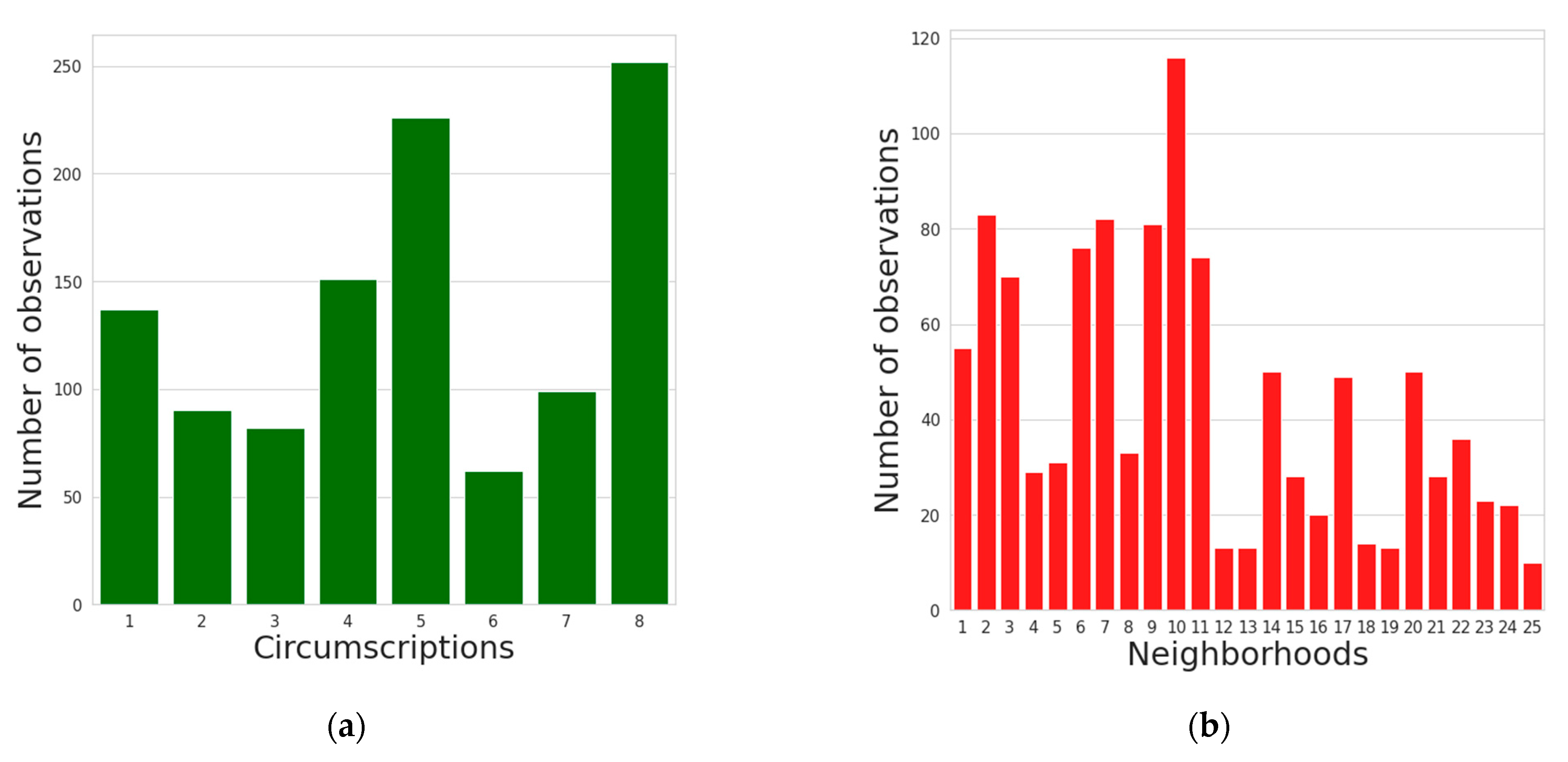
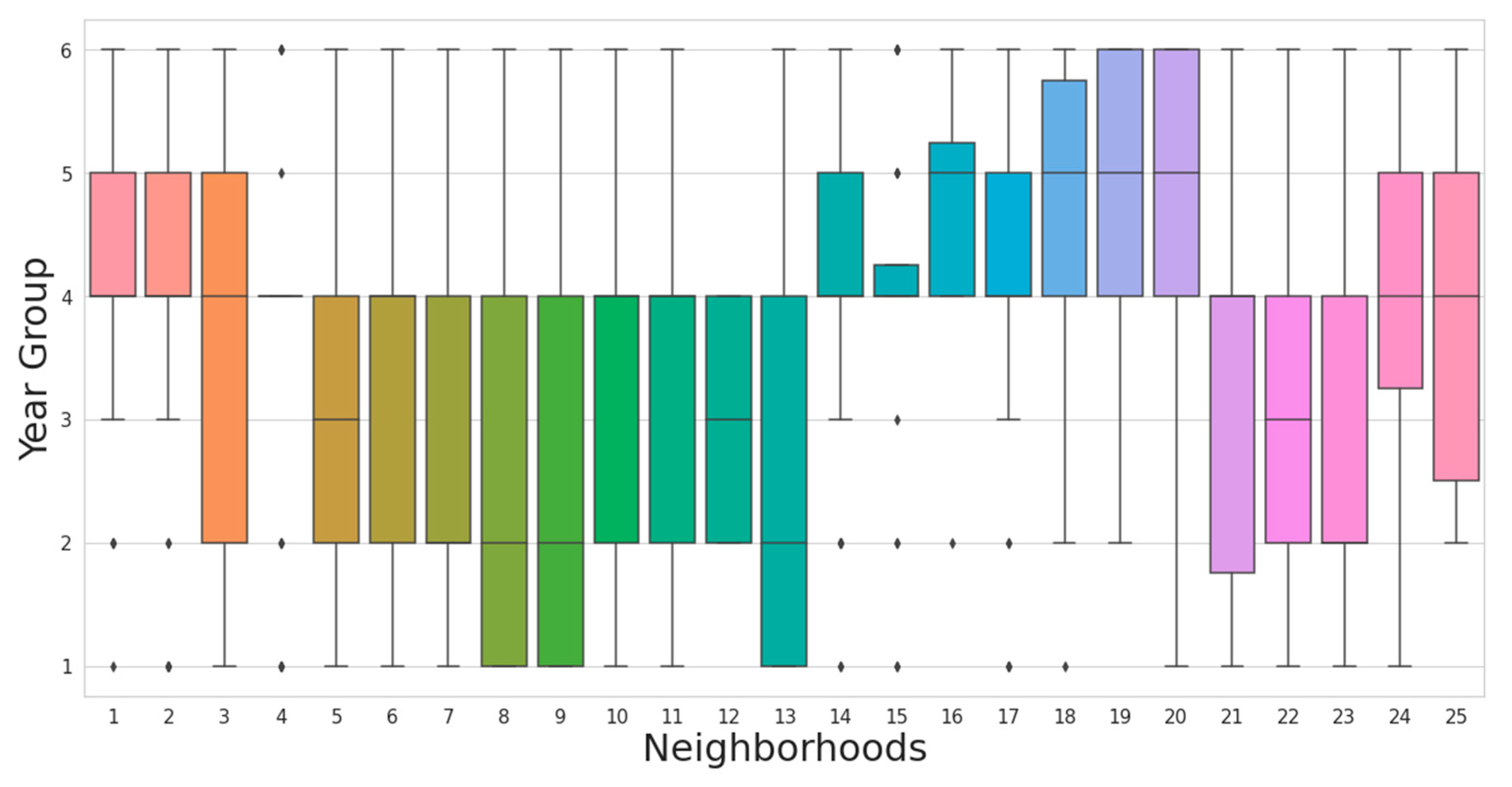
| neighborhood | neighborhood where the road is located |
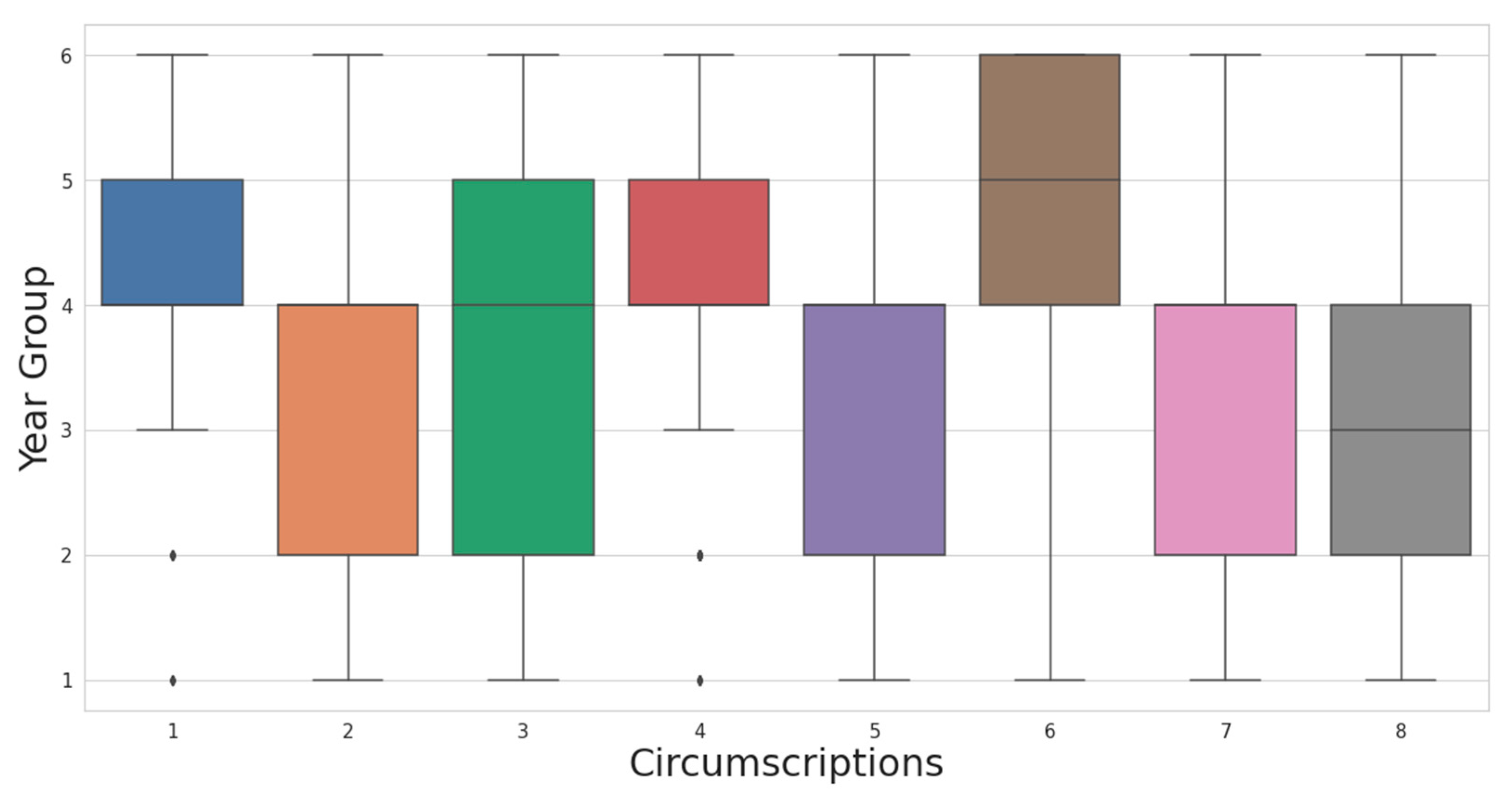
| circ | Circumscription (circ.) where the road is located |
| circ_pop | population of circ. where the road is located |
| street_category | road category classification (labelled 1 or 2; where 1 represents the higher trafficked option) |
| length | road length (measured in meters) |
| area | road area covered (measured in sq. meters) |
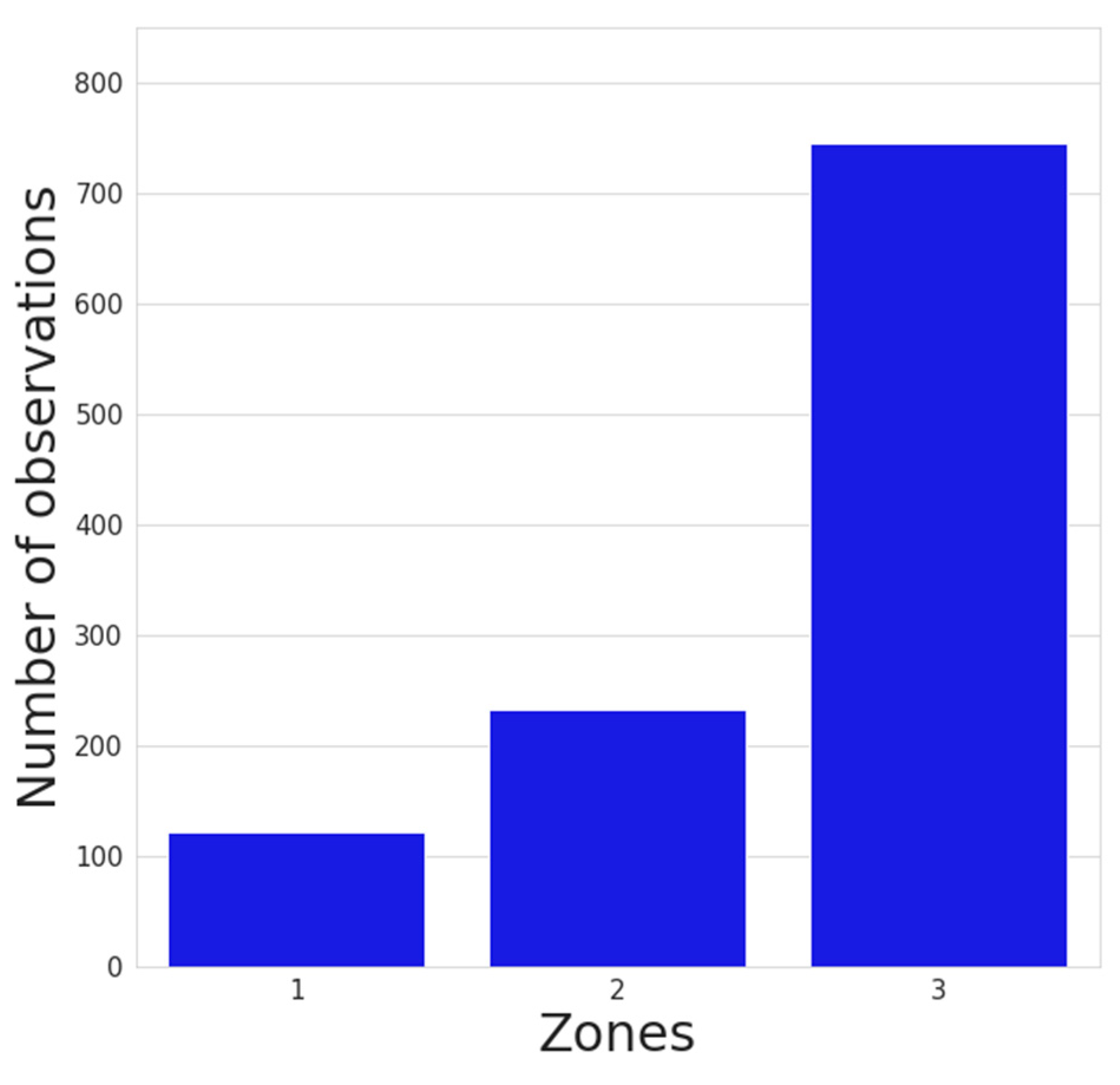
| zone | zone where road is located (1-historic center, 2-main city, 3-peripheries) |
| year | year group of maintenance |
| pop_den | density of population in circ. |
| public_buildings | The presence or lack of public buildings near the road (labelled 1 for yes and 0 for no) |
| commercial_activties | The presence or lack of commercial activities along the road (labelled 1 for yes and 0 for no) |
| traffic_rate | rate of activities in traffic zone where the road is located |
| tz_pop | population of traffic zone where the road is located |
| tz_pop_den | population density of traffic zone where the road is located |
| tz_workers | number of workers in the traffic zone where the road is located |
| unemployment | percentage of unemployment in circ. where road is located |
| industrial_jobs | percentage of industrial jobs in circ. |
| circ_road_den | road density within circ. where road is located |
| t_arrivals | number of trip arrivals in the traffic zone where the road is located |
| tz_departures | number of departures in the traffic zone where the road is located |
| tz_perdays_rt | number of total trips made within the traffic zone where the road is located |
Publisher’s Note: MDPI stays neutral with regard to jurisdictional claims in published maps and institutional affiliations. |
© 2021 by the authors. Licensee MDPI, Basel, Switzerland. This article is an open access article distributed under the terms and conditions of the Creative Commons Attribution (CC BY) license (http://creativecommons.org/licenses/by/4.0/).
Share and Cite
Roberts, R.; Inzerillo, L.; Di Mino, G. Exploiting Data Analytics and Deep Learning Systems to Support Pavement Maintenance Decisions. Appl. Sci. 2021, 11, 2458. https://doi.org/10.3390/app11062458
Roberts R, Inzerillo L, Di Mino G. Exploiting Data Analytics and Deep Learning Systems to Support Pavement Maintenance Decisions. Applied Sciences. 2021; 11(6):2458. https://doi.org/10.3390/app11062458
Chicago/Turabian StyleRoberts, Ronald, Laura Inzerillo, and Gaetano Di Mino. 2021. "Exploiting Data Analytics and Deep Learning Systems to Support Pavement Maintenance Decisions" Applied Sciences 11, no. 6: 2458. https://doi.org/10.3390/app11062458
APA StyleRoberts, R., Inzerillo, L., & Di Mino, G. (2021). Exploiting Data Analytics and Deep Learning Systems to Support Pavement Maintenance Decisions. Applied Sciences, 11(6), 2458. https://doi.org/10.3390/app11062458