Article

Implementation of Machine Learning Algorithms in Spectral Analysis of Surface Waves (SASW) Inversion

by
Sadia Mannan Mitu
1,
Norinah Abd. Rahman
1,*,
Khairul Anuar Mohd Nayan
2,
Mohd Asyraf Zulkifley
1 and
Sri Atmaja P. Rosyidi
3
1
Faculty of Engineering and Built Environment, Universiti Kebangsaan Malaysia, Bangi UKM 43600, Malaysia
2
Virtual Instrument & System Innovation Sdn Bhd, Petaling Jaya 47301, Malaysia
3
Department of Civil Engineering, Universitas Muhammadiyah Yogyakarta, Jalan Brawijaya (Lingkar Selatan), Bantul, Yogyakarta 55183, Indonesia
*
Author to whom correspondence should be addressed.
Appl. Sci. 2021, 11(6), 2557; https://doi.org/10.3390/app11062557
Submission received: 22 February 2021 / Revised: 6 March 2021 / Accepted: 7 March 2021 / Published: 12 March 2021
(This article belongs to the Special Issue Artificial Neural Networks Applied in Civil Engineering)

Abstract

:
One of the complex processes in spectral analysis of surface waves (SASW) data analysis is the inversion procedure. An initial soil profile needs to be assumed at the beginning of the inversion analysis, which involves calculating the theoretical dispersion curve. If the assumption of the starting soil profile model is not reasonably close, the iteration process might lead to nonconvergence or take too long to be converged. Automating the inversion procedure will allow us to evaluate the soil stiffness properties conveniently and rapidly by means of the SASW method. Multilayer perceptron (MLP), random forest (RF), support vector regression (SVR), and linear regression (LR) algorithms were implemented in order to automate the inversion. For this purpose, the dispersion curves obtained from 50 field tests were used as input data for all of the algorithms. The results illustrated that SVR algorithms could potentially be used to estimate the shear wave velocity of soil.

1. Introduction

The spectral analysis of surface waves (SASW) method is a nondestructive technique used to determine the shear wave velocity of layered material by using the theory of stress wave propagation. This method employs the dispersive characteristics of Rayleigh waves to determine the variation of stiffness with depth. Rayleigh waves propagate along a cylindrical wavefront near the surface of a half-space, and the amplitude of particle motion decays exponentially with depth [1]. Rayleigh waves disseminate two thirds of energy for a vertical load in a homogeneous isotropic half-space [2]. Rayleigh wave phase velocity primarily depends on the material properties, specifically shear wave velocity, compression wave velocity, Poisson’s ratio, and mass density to a depth of one wavelength, as shown in Figure 1. In geotechnical engineering, the SASW method has been used extensively to determine the various parameters of soil, such as bearing capacity [3,4,5], small stiffness [6], and pavement subgrade stiffness [7].
One of the complex processes in SASW data analysis is the inversion procedure. Studies related to the inversion procedure can go in many directions due to the procedure’s complexness, which includes generation of the theoretical dispersion curve method, simplification of the procedure, problems with multi modes of the dispersion curve, and nonuniqueness of the solution. Nazarian [9] used a modification of the Haskell–Thomson technique [10,11] to generate the theoretical dispersion curve. He employed the INVERT program, which is computer software designed for assuming the initial stiffness profile reported by Ballard [12], to compare the shear wave velocities directly. The differences between the shear wave velocity profiles from Ballard’s results and those from the Nazarian study were quite drastic. Therefore, the simplified inversion process based upon scaling the dispersion curve employed by many researchers is not suitable. Hossain and Drnevich [13] found some limitations in Nazarian’s technique. The method used to find the roots of the characteristics determinant for a layered system is quite complicated. Another limitation is the trial-and-error process of matching the theoretical and experimental dispersion curves. Hossain and Drnevich applied two methods, using the FORTRAN 77 program to determine the pavement moduli and thicknesses to overcome these difficulties, while they later developed a finite difference technique to analyze the generalized Rayleigh waves in multilayered elastic media. This method is very significant when it comes to determining the theoretical dispersion curve for a pavement system, which leads to a quadratic eigenvalue problem for the pavement system and a linear eigenvalue problem for the geologic model. The second technique comprised using a modification of Knopoff’s [14] algorithm to determine the theoretical dispersion curve. Later on, Yuan and Nazarian [15] generated an algorithm based on the energy integral equation to overcome this problem. Moreover, Addo and Robertson [16] developed a unique SASW system requiring no spectrum analyzer. Microcomputerization was used to conduct the entire procedure, and is able to determine the in situ dispersion curve. A program called “SASWFM” was written to automate the inversion process. The shear wave velocity can be obtained directly from the experimental dispersion curve. The results were compared to Seismic Cone Penetration Testing (SCPT) tests and reflected a relatively poor match between the experimental curve and the theoretical dispersion curve in some of the sites. Overall, the microcomputer-based system reduces the time for testing and the cost of equipment. To overcome the difficulties associated with the presence of multiple modes in SASW signals, Zomorodian and Hunaidi [17] introduced a new inversion method based on the maximum vertical flexibility. Meier and Rix [18] proposed the back-calculation neural network to replace the intensive computation of trial and error and the least-squares inversion method. Studies related to SASW inversion are summarized in Table 1.
The complexity of the SASW method in terms of data reduction has encouraged researchers to find a much more straightforward alternative without relinquishing reliability. Another motivation for much simpler analysis is to make SASW available for all users, be they experienced or beginners. Recently, a guideline for nonexpert users in surface wave acquisition and analysis has been published by Foti et al. [19]. The guideline presented a wide range of concerns related to the surface wave technique, including the nonuniqueness problem of SASW solutions.
In conventional SASW inversion analysis, a soil profile needs to be assumed for the inversion process, which involves calculating the theoretical dispersion curve by means of forward modeling [24]. A misfit between the experimental curve and the theoretical dispersion curve is then iteratively and automatically minimized to a predefined small value. If the assumption of the starting soil profile model is not reasonably close, the iteration process might lead to nonconvergence or take too long to be converged. Therefore, each step in the inversion process requires careful execution. Expert user opinions are often necessary in order to dispose of uncertain interpretation of the shear wave velocity profile and define the criteria for a final profile. To improve the complexity of the inversion process, some machine learning (ML) algorithms were proposed in this study. The main objective of the present study is to accelerate and simplify the inversion process by training the selected ML algorithms to ‘understand’ how conventional SASW inversion comes out with a shear wave velocity profile from the corresponding experimental dispersion curve, as illustrated in Figure 2.
An artificial neural network (ANN) is a popular ML model which has been adopted in recent years to automate the SASW inversion method [23,25,26,27]. Williams and Gucunski [23] determined the moduli and thicknesses of a four-layered pavement system through the use of an ANN. Later, Gucunski et al. [27] improved the models to develop five ANN models, with each model determining one single property of the pavement system. Shirazi et al. [25] developed a number of different ANN models to automate the SASW method in pavements. They used several points of the dispersion curve as input and the thicknesses and the elastic moduli of the layers as output. Three ANN software packages (STATISTICA, ANN toolbox by MATLAB, and NeuralSIM) were employed and the models could generate reasonably close elastic modulus for the upper layers. Alimoradi et al. [26] used the results of the SASW tests to train ANN for the classification of shear wave velocity. They conducted nine SASW methods and Downhole Tests (DHT) and determined the unknown nonlinear relationships between SASW results and those obtained by means of the method of DHT, the latter of which have been treated as real values. The results show that the backpropagation neural network could predict the shear wave velocity between wells accurately. Therefore, due to the performance of ANN in SASW inversion by previous researchers, an ANN model will be adopted in this study and compared to other ML algorithms.

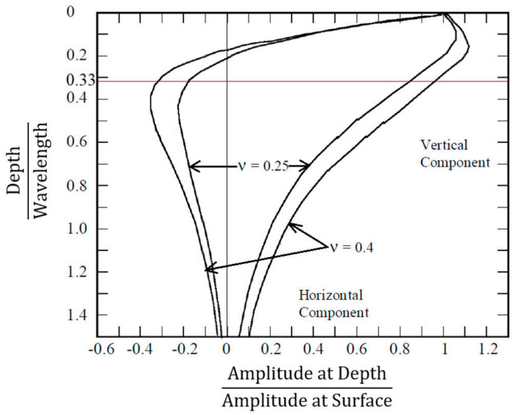
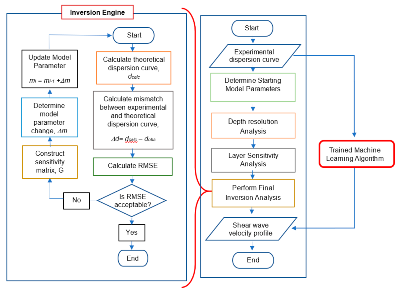
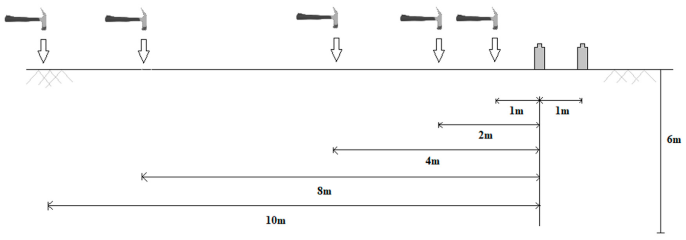
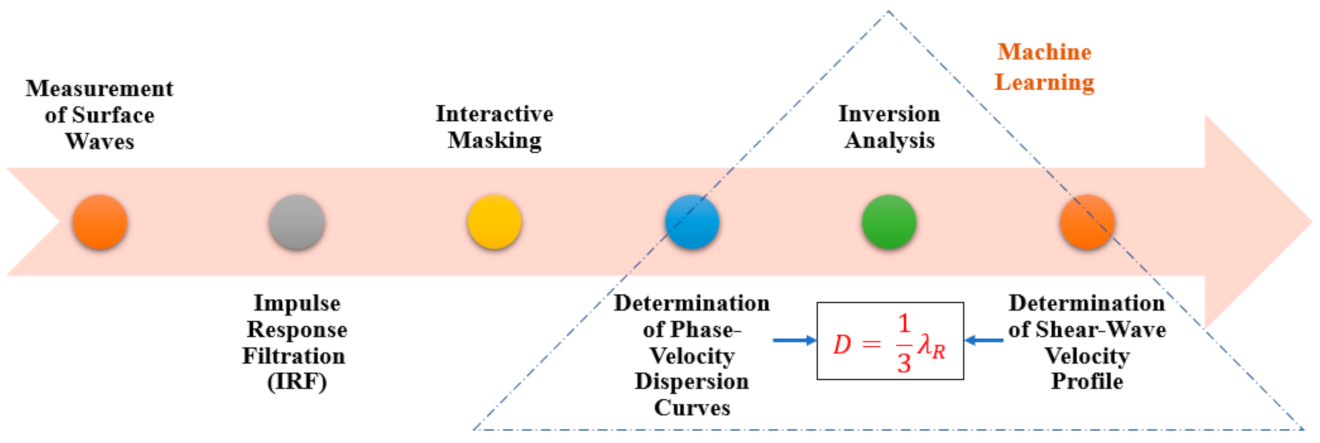
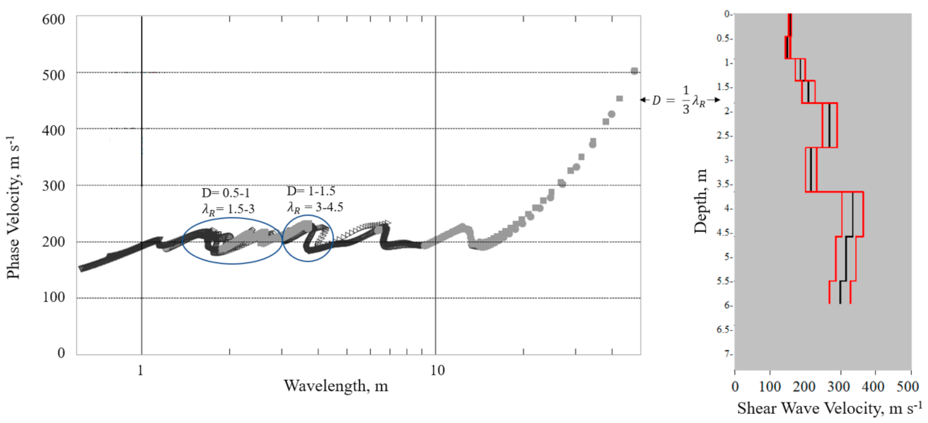
2. Inversion Analysis

The conventional inversion method used in the present study is described in this section. Determination of the Starting Model Parameter (SMP), depth resolution analysis, layer sensitivity analysis, and final inversion analysis are the major steps in the inversion procedure, as shown in Figure 2 (on the right-hand side of the flow diagram). Firstly, the SMP was determined based on the theoretical dispersion curve and the assumption of the parameters. An assumption of the number of layers, as well as of each layer’s thickness, was made for the iterative procedure [15]. Subsequently, depth resolution analysis and layer sensitivity analysis refined the starting model in the first step. Several iterations are required for the steps of refining the starting model. These three steps constitute the preliminary inversion analysis. After completing the preliminary inversion analysis, the final inversion analysis, which has been denoted as Inversion Engine in the flow diagram, can be performed.
The starting model is called a preliminary shear wave velocity profile, since shear wave velocity is used as a model parameter for the inversion procedure. There are two steps involved in constructing the preliminary shear wave velocity profile. A preliminary shear wave velocity profile is determined as the first step. Based on the experimental dispersion data distribution, layer thicknesses and the number of layers are calculated for the preliminary profile. In the second step, another profile is determined from the preliminary profile based on the layering determined in the first step. The second profile is used for the inversion analysis.
The measurement of depth resolution evaluates the optimum resolvable depth for a given experimental dispersion curve [24]. The deepest resolvable layer is dependent on the penetration depth or the zone stressed by the surface wave. The penetration depth is influenced by the frequencies generated by the source on the surface and the stiffness structure of the subsurface. Inversion analysis is very reliant on the layering of the starting model. Layering of the subsurface structure is assumed initially for the inversion technique. Consequently, a measure must be provided so as to indicate how good the assumed layering is. Layer sensitivity analysis decides whether or not the assumed layering is suitable. The assumed layering could be improved to provide a proper resolution, depending on the layer sensitivity analysis [24].
The inversion engine, as illustrated in Figure 2, represents the principal flow of the inversion analysis. This engine has two components: one calculates root mean square error (RMSE), and the other updates the model parameters. The parameters include shear wave velocity, Poisson’s ratio, compression wave velocity, mass density, and the material damping ratio [28]. Wave velocities are updated for every iteration; however, the parameters, such as Poisson’s ratio, mass density, and the material damping ratio, are reasonably assumed, since their effect on phase velocity is considerably small. Compression wave velocity is explicitly related to shear wave velocity and Poisson’s ratio. Thus, it can be calculated using the assumed Poisson’s ratio and the updated shear wave velocity. Therefore, only shear wave velocity was used as the modal parameter for the inversion analysis. The sensitivity matrix, G, and the change in a model parameter, ∆ m , are determined to update the model parameters.
After completing the preliminary inversion analysis, the final inversion analysis can be performed. Iteration of the inversion analysis is continued until the theoretical dispersion curve is similar enough to the experimental dispersion curve [29]. RMSES measures the misfit between the theoretical curve and the experimental dispersion curve and evaluates the goodness of the shear wave velocity profile. Subscript ‘S’ is added to the abbreviation of RMSE to distinguish the misfit in dispersion curves from RMSE in ML training. Lower RMSES are considered the best match between the theoretical and experimental dispersion curves [30]. Since iteration is incorporated into the inversion analysis, there must be a measure with which to quantify the goodness of the estimated model parameters and the predicted shear wave velocity. The prediction error can be defined in several ways, but the maximum likelihood approach for the inversion analysis justifies the use of the L2 norm, which is a loss function that reflects least-squares errors, as defined in Equation (1). The maximum likelihood approach is one of the procedures used to find the optimum shear wave velocity for an experimental dispersion curve:
L 2 n o r m :   e 2 =   i e i 2
where e i is the difference between the observed data and the shear wave velocity. The RMSEs in Equation (2) is a representation of the L 2 norm. The RMSEs is independent of the number of datasets and provides the absolute sense of the average misfit:
R M S E s =   1 n i e i 2
where n is the number of datasets and i represents the variables.
Evaluation of a stiffness profile requires an experimentally determined phase velocity dispersion curve which is produced via iterative forward modeling analysis or inversion analysis [15,31]. This inherent problem of inversion analysis requires several tries of an initial guess or a reasonable initial guess. To simplify this inversion process, the experimental dispersion curve and the final shear wave velocity were used to train the ML algorithm, as indicated in Figure 2.

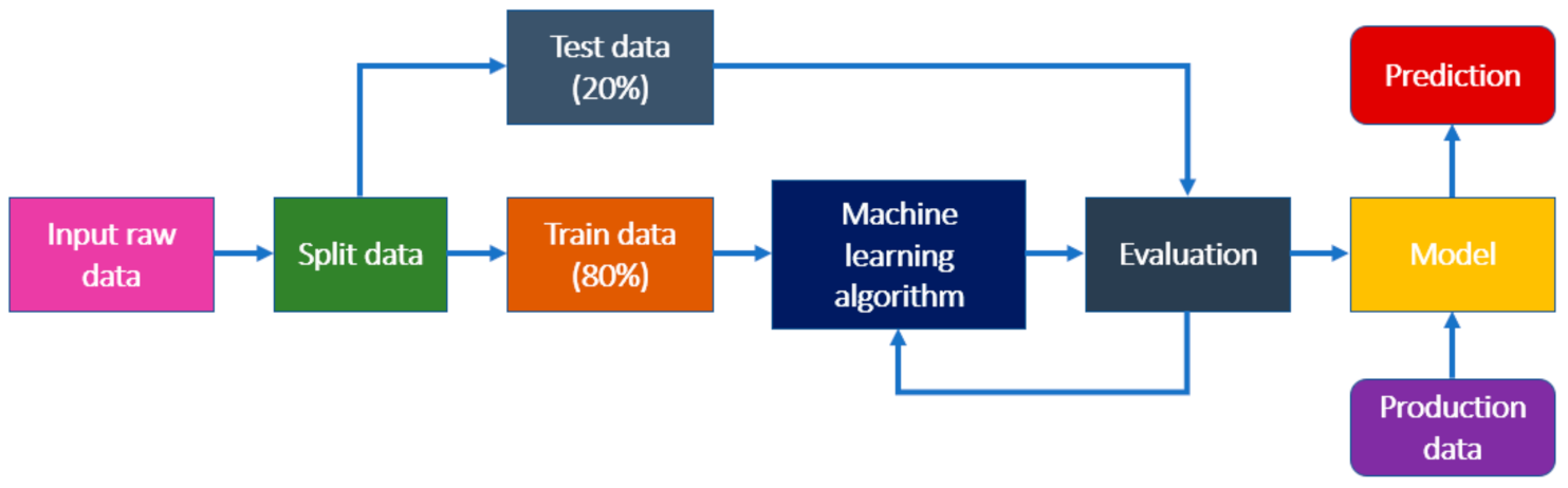
3. Machine Learning (ML) Algorithms

Machine learning (ML) is an application of artificial intelligence which is able to perform tasks by observing several previous examples and information without being programmed. To predict the shear wave velocity profile from the experimental dispersion curve, an ANN known as MLP was adopted in this study. The predictive performance of the ANN is then compared with other ML algorithms, namely RF, support vector machine (SVM), and LR. An overview of each algorithm, such as their unique features and advantages that motivate their use in this study, is put forth in the present section. Since the dataset from the SASW inversion consists of a set of inputs and outputs, all algorithms chosen are supposed to be supervised ML algorithms. The workflow of a supervised ML model is shown in Figure 3.

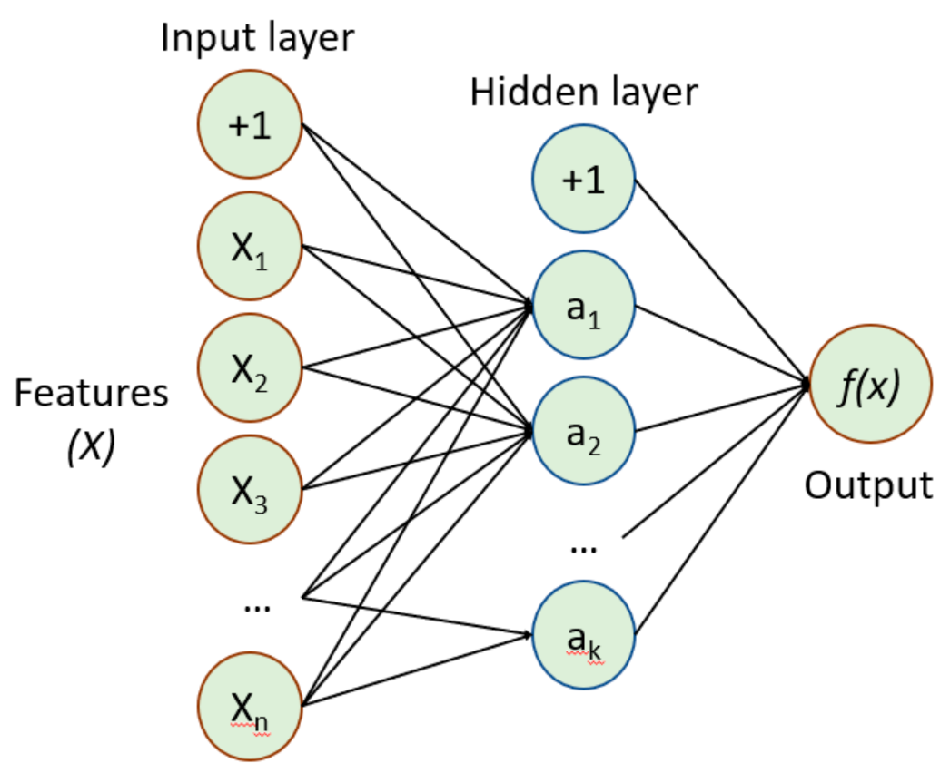
3.1. Multilayer Perceptron (MLP)

Multilayer perceptron (MLP) is a class of feed-forward ANN. The structure of MLP includes an input layer, an output layer and a hidden layer. This algorithm learns a function, f : R n R o , by training on a dataset, wherein n is the number of inputs and o is the number of outputs. There can be several hidden layers in the MLP algorithm. Figure 4 shows the MLP network with one hidden layer.
The set of neurons { x i | x 1 ,   x 2 , , x n } is the representation of the input layer, which is raw data collected from the field. The hidden layer transforms each neuron from the input layer with a weighted linear summation w 1 x 1 + w 2 x 2 + + w m x m, followed by a nonlinear activation function g : R R , such as the hyperbolic tan function. Thereafter, the output receives the values from the last hidden layer.

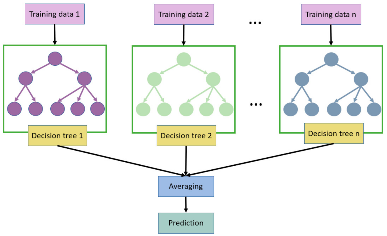
3.2. Random Forest (RF)

Random forest (RF) is an effective model for predictive analysis, as it uses ensemble learning methods for classification and regression [32]. However, fine-tuning of its hyperparameters is required by optimization algorithms for excellent RF modeling. This algorithm has been employed for solving geotechnical engineering problems by, for example, assessing pile drivability [33], the undrained shear strength of soft clays [34], and liquefaction potential [35]. RF regression is based on decision trees for creating predictive models. Each tree is trained on a randomly sampled subset of the input data. If a training dataset is used as input with targets and features in the decision tree, the algorithm will formulate some set of rules. Each tree works individually, with no interaction happening between them. The RF model splits the nodes in each tree, considering a limited number of features, and combines hundreds or thousands of decision trees. Thereafter, the results are predicted based on the average predictive value of each tree. Figure 5 is a representation of the RF decision trees.

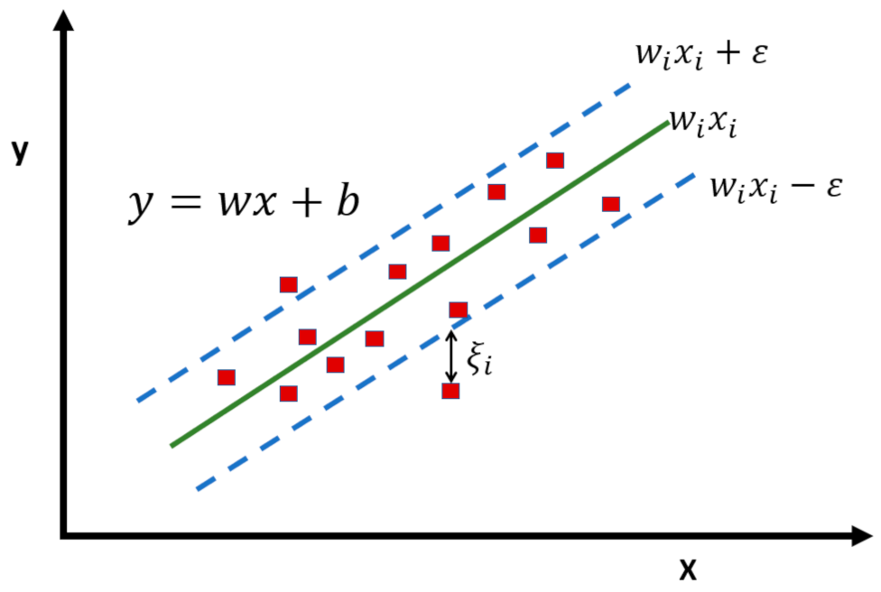
3.3. Support Vector Machine (SVM)

The support vector machine (SVM) is a supervised ML algorithm that predicts a model significantly with less computational power [36]. It can be used for both regression and classification tasks [37]. SVR is derived from the SVM and is a prediction method that utilizes the principle of ML to optimize prediction precision while preventing overfitting the data automatically. Rather than the conventional empirical risk minimization (ERM) principle, the SVM is trained using the systemic risk minimization (SRM) principle [38]. Only the errors associated with the training dataset are minimized by means of ERM, but SRM simultaneously minimizes the empirical risk and model complexity. In other words, a tradeoff between the consistency of the approximation of the model and the sophistication of the approximation function is implied by the SRM principle. SVR thus prefers smooth models that do not overfit the training data—a requirement for successful unseen (testing) data generalization capabilities.
The principles of SVR are similar to the SVM for classification, but there are a few differences between them. It requires a set of inputs and corresponding outputs to predict the model. The SVM finds a hyperplane in some features which separates the data points into two classes [39]. Many hyperplanes could be chosen to separate the data points. This choice can be made by observing the maximum margin distance between the data points of both classes. Samples on the margin are called support vectors. SVR finds a function f x that has the most deviated margin of tolerance ε from the actual target value   y for all of the training data. The linear function is defined as Equation (3):
f x   =   w ,   x +   b
where x is used to estimate the scaler vector of y by means of the n-dimensional weighting coefficient w , and the constant coefficient is b . The margin of tolerance can be minimized and calculated as:
m i n i m i z e   1 2   w 2   +   C i = 1 n ε i
It is assumed that the function f estimates all of the pairs x i , y i with precision through the use of Equation (4). If the data cannot be placed into the margin, the slack variables ξ i can be used to solve the problem via Equation (5):
y i     w i x i     ε   + ξ i
Figure 6 graphically depicts the linear SVR. Generally, four types of kernels are used in the SVR models, namely linear, polynomial, radial basis function (RBF), and sigmoid. The mathematical representation of each kernel is given in Equation (6) [40]:
K X i ,   X j =   X i X j                                                                                         L i n e a r γ X i X j + C d                                   P o l y n o m i a l exp γ X i X j 2                                         R B F t a n h γ X i X j + C                                   S i g m o i d
where K X i ,   X j represents the kernel functions and γ and d denote the kernel width and the power exponent, respectively. Here, C is the kernel parameter. In this study, the RBF was used. The RBF is the most popular kernel type used in SVR because of its localized and finite responses across the entire range of the real x-axis [41].

3.4. Linear Regression (LR)

Linear Regression (LR) is the simplest ML algorithm that performs only regression tasks. LR predicts a dependent variable value based on a given independent variable. The algorithm creates a linear relationship between input and output. The model finds the best line of fit based on the minimum error between the predicted and observed values. The hypothesis function for LR is given in Equation (7):
Y   =   θ 0 +   θ 1 x 1 +   θ 2 x 2   + + θ n x n
where Y is the predicted value, θ0 is the bias term, θ1, …, θn are the model parameters, and x1, x2, …, xn are the feature values. The aforementioned hypothesis can also be represented by Equations (8) and (9):
Y   =   θ T x
f i θ =   θ T x + i
where f i θ is the hypothesis function and i is noise. An intercept term is added by appending a column of 1 s to the features. Regularization is often required in order to prevent overfitting by penalizing models with extreme parameter values. The LR model supports L1 and L2 regularization, which are added to the loss function [42]. The L1 norm can be determined from the sum of the absolute values of the vector, and the L2 norm can be obtained as the square root of the sum of the squared vector values that are used to minimize the error. One of the main mysteries revealed by deep learning methodology is the concept of benign overfitting: deep neural networks tend to predict well, even with a perfect match for noisy training results. This algorithm was used to predict shear wave velocity at 30 m by means of a 95% confidence interval [43]. Therefore, LR is considered in this study, albeit a simple ML algorithm.

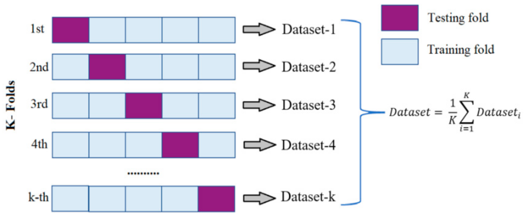
3.5. K-Fold Cross-Validation

The primary goal of cross-validation is to avoid the bias of an algorithm in training and testing data selection. The process estimates the performance of ML algorithms based on unseen data or the data not in use during the training. It is called k-fold cross-validation. The parameter k refers to the number of datasets into which a given data sample is to be split, as shown in Figure 7. Each dataset is split into 80% for training and 20% for testing purposes.

4. Methods and Materials

In the SASW method, Rayleigh waves are generated by any impact source and detected by two receivers before then being recorded by a spectrum analyzer, as shown in Figure 8. Rayleigh wave data were collected and transformed into the frequency domain through the use of a dynamic signal analyzer [44].
The seismic experiments (SASW) were carried out at 50 different locations in Peninsular Malaysia. SASW data are from a broad collection of geological and geotechnical site conditions ranging from recent alluvium, granitic to metasedimentary formations with geotechnical consistency of soft/loose to hard/dense soil conditions. The dispersion curves of all 50 corresponding sites can be found in the appendices. During the tests, both geophones were placed 0.5 m away from the specific points so as to maintain a 1 m distance between said geophones.
A rubber hammer, a geological hammer, a sledgehammer and a 10 kg weight were used to hit the soil surface in order to produce a transient vertical impact. Sources were placed at 1, 2, 4, 8, and 10 m from the first geophone, as shown in Figure 9. Thereafter, the data obtained from the field were analyzed using WinSASW 3.2.12. The depth was taken up to 6 m in dataset preparation for ML algorithm training and testing. The range of wavelengths of the dispersion curve needs to include the wavelengths for sampling shallow material and be long enough to penetrate deep layers. One source and receiver’s setup are not sufficient to determine phase velocities over a wide range of wavelengths, which is required to evaluate a soil site with a depth of, for example, 30 ft (9 m) to 60 ft (18.3 m). Therefore, several measurement setups comprising different receiver spacings are used for this purpose.
Figure 10 illustrates the summary of the SASW data analysis and the implementation of the ML through the use of the SASW method. The first task in analyzing the field measurements is the construction of an experimental dispersion curve. It is important to unwrap the phase spectrum in order to accomplish this task. An interpretation of the phase spectrum is required so as to unwrap the phase spectrum. The technique is called masking for interpreting the phase spectrum. The unwrapped phase spectrum and the receiver spacing determine the experimental dispersion curve by means of Equation (10):
V P H = f .   λ
V P H = f .   d φ / 360 °
where φ is the phase difference between the two receivers for the wave traveling with the frequency of f , and d is the distance between the two receivers.
The material properties and thickness of the soil profiles were assumed to obtain the theoretical dispersion curve. The soil layers were assumed to comprise 12 layers of 0.5 m thickness, a bulk density of 1800 kg m−3, a Poisson’s ratio of 0.3333, and a damping ratio of 0.02. The theoretical dispersion curve was generated based on this assumed parameter. Thereafter, the theoretical dispersion curve and the experimental dispersion curve obtained from the field were compared.
The triangular part of Figure 10 is explained in detail in Figure 11. The parameters considered in the development of the ML were the shear wave velocity ( V S ) , thickness, wavelength, and phase velocity of each layer. The theoretical dispersion curves from 50 tests were taken as input. A total number of 4782 data points was found from the 50 dispersion curves. Subsequently, all of the measurements obtained from the dispersion curve were divided into 12 layers of 6 m depth at a 0.5 m interval, as shown in Figure 11. The wavelengths were converted to an equivalent depth of 1 3 λ R . For every 0.5 m of depth, D, the wavelength, λ R , was calculated using Equation (11):
D =   1 3 λ R
As shown in Figure 11, the wavelength starting from 1.5–3 m belongs to 0.5–1 m layers of depth. Similarly, the wavelength starting from 3–4.5 m belongs to 1–1.5 m layers of depth, and 16.5–18 m of the wavelength belongs to 5.5–6 m of depth. Afterwards, all of the dispersion curves from the 50 SASW tests were combined and divided into these 12 layers at a 0.5 m interval. For training the datasets, the wavelength and the phase velocity were considered to be input corresponding to each layer. For instance, the wavelengths from 0–1.5 m were taken as input, as well as the shear wave velocities at 0–0.5 m depth. The theoretical dispersion curves, along with the soil profile from the database, were used to train the ML algorithms. The proportion of the training and testing datasets was 80% and 20%, respectively, in the ML algorithms. The contention was to generate the most extensive, theoretically possible input range.
The number of observations obtained from the dispersion curve at different layers is shown in Table 2. The deepest resolvable layer is related to the penetration depth of the surface wave. The penetration depth is controlled by the frequencies generated by the source on the surface and by the stiffness structure of the subsurface. The surface wave needs to propagate deeper with the right range of low frequencies in order to be able to capture the deep layer. Generally, hammer impact sources have a limitation in low-frequency generation in comparison to higher-frequency generation. Therefore, the data points obtained from the field decrease with deeper layers. To evaluate the V S profile from the SASW measurements, dispersion curves must be determined.
To measure the performance of the model, the coefficient of determination (R2) and RMSE were used. Equation (12) is employed to determine the RMSE in the ML algorithms:
R M S E =   i = 1 N ( P i     A i ) N
where P i is the predicted shear wave velocity, A i is the shear wave velocity from conventional SASW inversion, and N is the sample size.
The following parameters in Table 3 were used in ML for the algorithms.

5. Results and Discussions

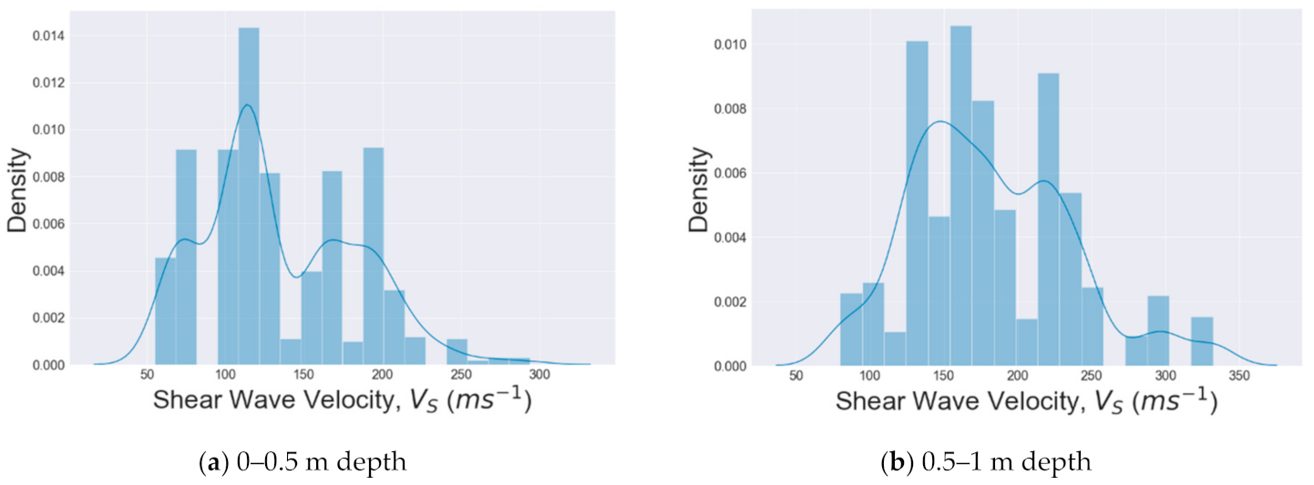
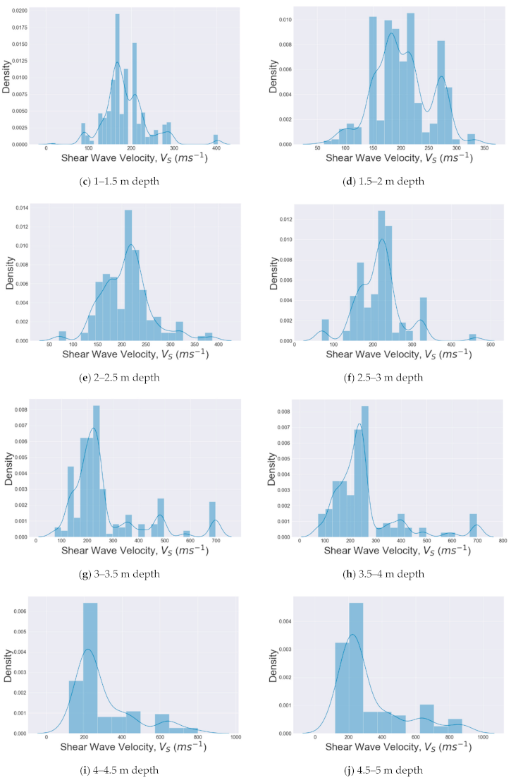
5.1. Distribution of Datasets

The most important step is to determine the underlying distribution of data before applying any ML approach. In an ML context, the input data for processing comprise only numerical values. A histogram is a visual representation of the dataset distribution that shows any outliers or gaps in the data. ML performance depends on the distribution of the datasets. If the data distribution is not normal, then it can be skewed to the left or right or be completely random. Whether or not the shear wave velocity obtained from the field is normally distributed is discussed below.
After analyzing Figure 12a–l, it can be concluded that all of the datasets after 3 m are positively skewed. Moreover, the layers are contaminated with the outliers found after 3 m of depth. Another observation from Table 2 is that the number of observations decreases with the increase of depth. However, a wide range of data points with the increase of depth can be observed in the histogram. Figure 12a illustrates the histogram of VS of 0–0.5 m depth. The histogram has a maximum value of 116.79 ms−1 and a minimum value of 0 ms−1. The frequency is zero within 81.36–90.21 ms−1 and 214.22–240.79 ms−1. Figure 12b illustrates the histogram of VS. at 0.5–1 m depth, and the majority of the values of shear wave velocity lie in the range of 120.47–250.67 ms−1. The frequency is zero between 258.81 and 275.09 ms−1. The maximum value of the third histogram (Figure 12c) is 173.71 ms−1, with the lowest being 0 ms−1. Two outliers at 12.06 and 402.7 ms−1 can be observed in the datasets. Besides, five nonfrequency ranges, from 12.06–92.89, 106.35–133.29, 200.65–214.12, 254.53–267.99, and 294.93–389.23 ms−1, can be found in the datasets. Figure 12d is the histogram of VS. at 1.5–2 m depth. This data can be defined as being normally distributed. The majority of the values of shear wave velocity lie in the range of 155.66–285.45 ms−1. No outliers can be observed in the dataset. The histogram of the VS. at 2–2.5 m depth is depicted in Figure 12e. It has one peak at 219.93 ms−1 and two gaps (zero frequency) within 86.47–136.52 and 336.7–353.38 ms−1. The histogram at 2–2.5 m depth follows a similar pattern to the fourth histogram. Figure 12f shows the histogram of the VS. at 2.5–3 m depth. There is one outlier at 459.79 ms−1 of VS.
The histogram of the VS at 3–3.5 m depth is emphasized in Figure 12g. These datasets are right or positively skewed. They also contain a significant number of outliers. The majority of the data can be found in the 206.65–251.24 ms−1 range, and the outliers are found from 429.6 to 697.14 ms−1. The histogram of VS at 3.5–4 m depth shows a similar pattern to the histogram at 3–3.5 m. The distribution of the datasets is also right skewed, as shown in Figure 12h. These datasets are contaminated with outliers detected from 322.59–697.14 ms−1. Figure 12i,j also depicts that the histogram of VS at 4–4.5 m and that of 4.5–5 m layers of depth are right skewed. Moreover, the outliers were detected from 421.46–799.44 ms−1 at 4–4.5 m and 455.36–875.71 at 4.5–5 m depth. Figure 12k,l illustrates that the VS histograms at 5–5.5 and 5.5–6 m layers of depth are right or positively skewed. Both layers are highly contaminated with the outliers detected from 857.49–1541.83 ms−1 at 5–5.5 m depth and 512.79–1361.85 ms−1 at 5.5–6 m depth. Therefore, it can be observed that the range of the VS started to increase from 3 m, going from 72.88–697.14 ms−1 at the seventh layer (3–3.5 m) and eighth layer (3.5–4 m). The range varies from 119.07–799.44 ms−1 at the ninth (4–4.5 m) layer and 100–900 ms−1 at the tenth (4.5–5 m) layer, while it goes from 173.17 to 1541.83 ms−1 for the last two layers (5–6 m), even though the number of observations is too low, at 77 and 60, respectively, in these layers (refer to Table 2). Real-time data are never usually normally distributed. In skewed data, the tail region may act as an outlier for a statistical model. Moreover, the outliers have an adverse effect on the model performance, especially on the regression-based models.

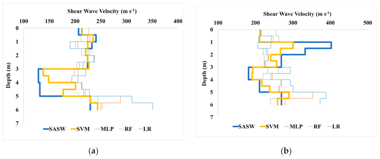
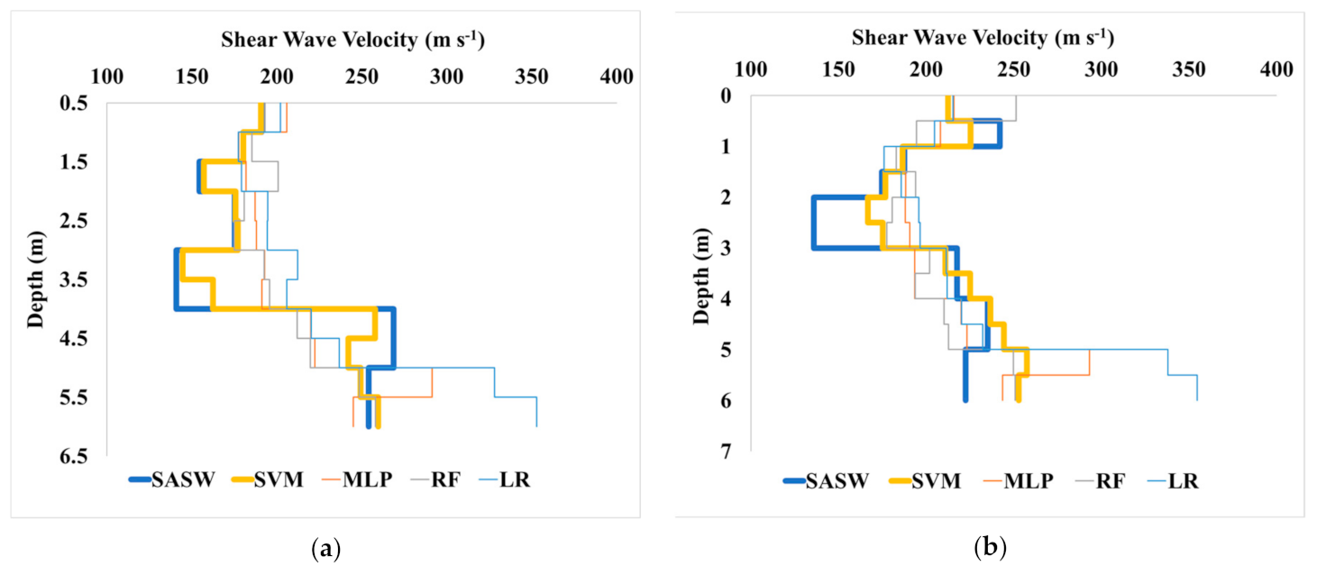
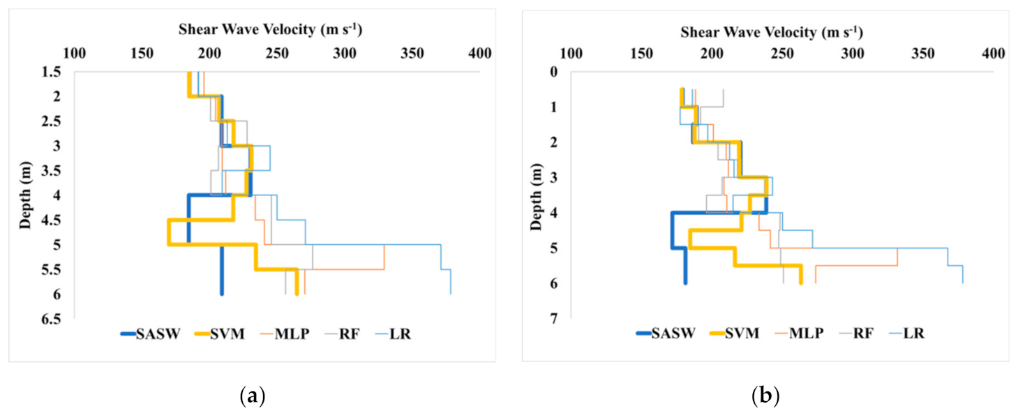
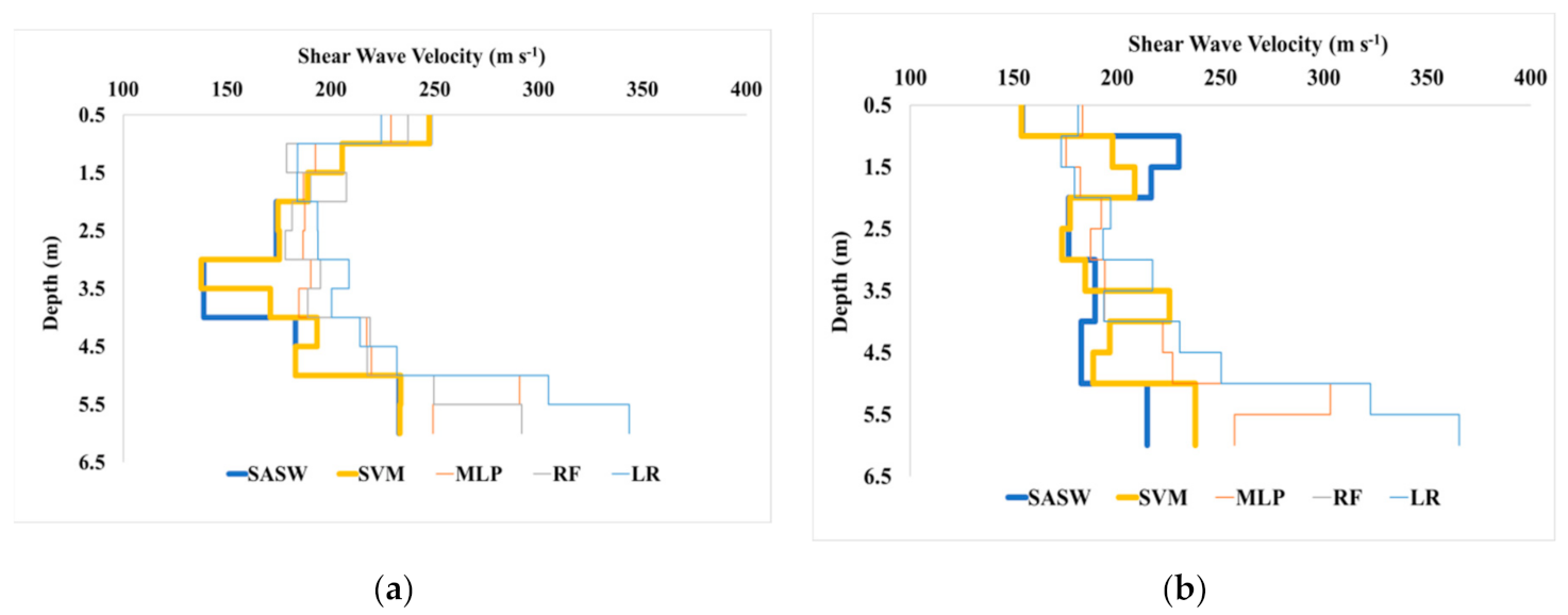
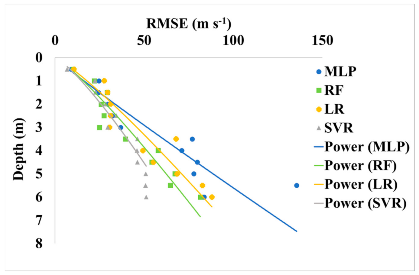
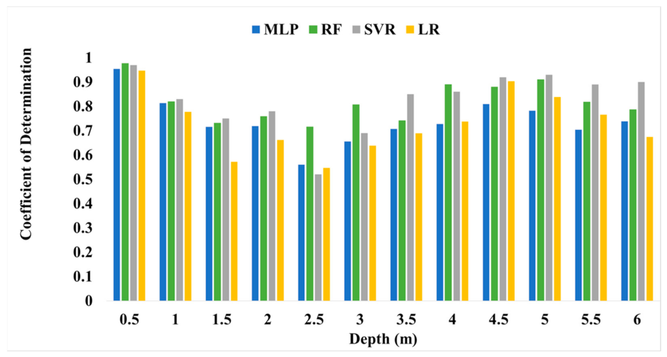
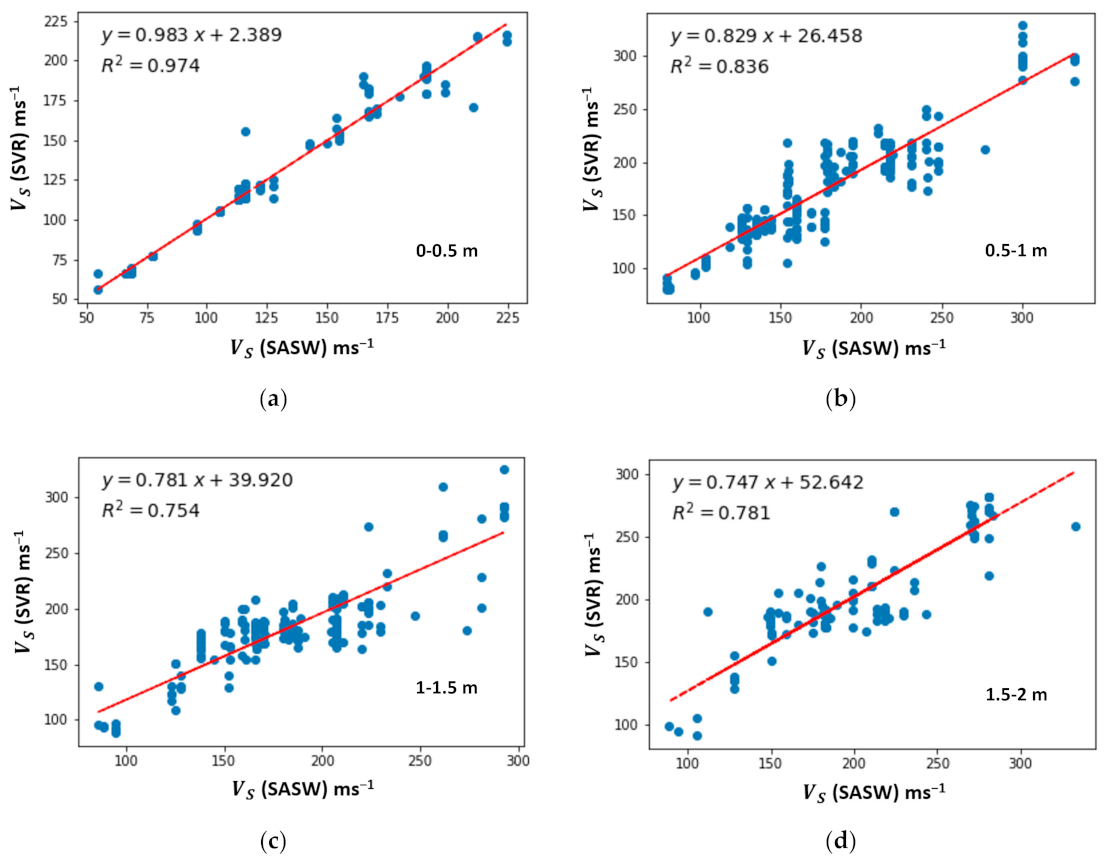
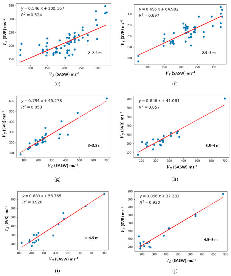
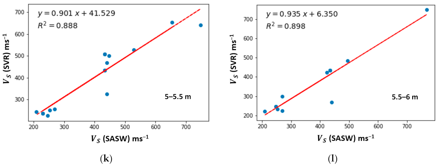
5.2. Comparative Analysis of Shear Wave Velocity for ML Algorithms

A comparison of the predicted shear wave velocity profiles from all ML algorithms with the shear wave velocity profiles from conventional SASW inversion is illustrated in Figure 13, Figure 14, Figure 15, Figure 16 and Figure 17. Each figure shows test 1 to test 10, respectively. Within the depth of 0.5 m, the V S obtained from conventional SASW is 206.7 m s−1, whereas the V S values obtained from MLP, RF, SVR, and LR are 213.01, 226.65, 213.25, and 213.74 m s−1, respectively, for test 1. Similarly, for the second layer, the V S values obtained are 240.73, 227.89, 211., 234.84, and 224.18 m s−1 from SASW, MLP, RF, SVR, and LR, respectively. The V S deviated at 4–5 m from the SASW value in test 1, as shown in Figure 13a. Figure 13b shows high similarity between SASW and SVR. However, a significant difference can be noticed over the depth interval of 1–2 m (up to 100 ms−1).
Figure 14a illustrates that the V S from SVR was close to the SASW values and continued up to 6 m. The V S from SVR was consistent throughout the depth. Figure 14b also shows significant similarities up to 6 m, but from 2–3 m, SVR drifted from the V S from SASW.
SVR showed notable results up to 6 m for Figure 15a,b and Figure 16a,b as well. The values obtained from the SVR deflected at the first layer for tests 5 and 6.
SVR makes quite a good prediction for test 9, as analyzed in Figure 17a. Furthermore, SVR predicts the V S profile quite well, except for the second layer (1–1.5 m) and seventh layer (3.5–4 m) for test 10, as illustrated in Figure 17b.
It is apparent from these figures that SVR has outstanding performance in comparison to the other algorithms in predicting shear wave velocities. A few drifts have occurred because there were insufficient data points to train in those layers. A comparison of the experimental data and the theoretical dispersion curve corresponding to the SASW profile is provided in the appendices in order to show what impacts this difference has on the effective theoretical dispersion curves that correspond to the shear wave velocity profiles from SASW and ML, and, subsequently, on how well they compare to the experimental data.
The confidence limit, percentage error, RMSE and R2 were measured for every layer (0–6 m depth) so as to produce a better evaluation of the ML algorithms.
Table 4 shows the confidence limit and the percentage error associated with the RMSE of composite values for the 10 test cases. It is visible that after 3 m depth, the confidence limit is lower than 80% in MLP, which is not reliable for design purposes [45]. The limit is found to be greater than 85% for SVR from 0–6 m depth. A detailed guideline on target confidence levels was provided by Lorig and Stacey [46]. Among all of the algorithms, SVR shows a better prediction, as the confidence limit is greater than 80%. Similarly, RF performs better, except for the last layer of depth. The highest percentage error is less than 15% for SVR, whereas it is greater than 20% for all algorithms.
The RMSE of composite values for the 10 test cases for different ML algorithms with conventional SASW inversion is shown in Figure 18. In the SVR algorithm the range of RMSE varies from 6.79 to 34.44 ms−1 up to 3 m, whereas in MLP it differs from 9.05 to 36.84 ms−1, in RF from 10.13 to 29.29 ms−1, and in LR from 10.66 to 31.20 ms−1. After 3 m, the RMSE nonlinearly increases with depth. For SVR, MLP, RF, and LR, the range of RMSE varies from 46.03 to 51.15 ms−1, 76.96 to 135.56 ms−1, 39.98 to 81.51 ms−1, and 49.28 to 87.95 ms−1, respectively. The resolution of shear wave velocity is not considerably good after the depth of 3 m. The distribution of datasets (refer to Figure 12) after 3 m of depth may cause a sudden increase of RMSE in the ML model.
R2 assesses how strong the linear relationship is between the conventional SASW and ML algorithms. Figure 19 represents the R2 of composite values for the 10 test cases. The R2 of RF, MLP, SVR, and LR is 0.98, 0.95, 0.97, and 0.95, respectively, for the 0–0.5 m layer, which is the highest value of R2. The lowest value is found to be 0.72 at 2–2.5 m depth for RF, 0.55 at 2–2.5 m depth for SVR, 0.52 at 2–2.5 m depth for MLP, and 0.55 at 2–2.5 m for LR. The R2 value of LR also decreases with depth but the value increases marginally at 4–4.5 m, and then begins to decline again.
The values of mean square error (MSE), RMSE, and R2 are given in Table 5.
In Figure 20a–l a schematic representation of the R2 of composite values for the 10 test cases between SVR and SASW can be analyzed. In the first layer (0–0.5 m), the R2 between SVR and SASW is high. The second layer (0.5–1 m) also reveals a strong association. The association between SVR and SASW is fairly high for the third layer (1–1.5 m) and the fourth layer (1.5–2 m). The R2 value is 0.85, which is a significant value at a depth of 3–3.5 m, including a few outliers, as seen in Figure 20g. The coefficient of determination increases significantly to 0.92 and 0.93 after 4 m, which is known to represent a good association between the shear wave velocity obtained from SVR and SASW, as seen in Figure 20i,j. At these layers, there are very few data points, and the distribution of the datasets can create a greater RMSE than the other layers.
Although an R2 close to 1 is a reasonable match, this value alone does not decide if the data points or predictions are biased. The performance also depends on the outliers and regression line, which is close to the points.
It can be concluded that the performance of SVR is better than that of the other algorithms when it comes to predicting the shear wave velocity. The other algorithms have high RMSE after 3 m of depth. Indeed, some outliers can be observed after 3 m of depth. The range of the datasets is broad, but the point that we obtain from SASW is low at this depth, which may affect the ML models.

6. Conclusions

Automation of SASW inversion was proposed in this study by adopting four ML algorithms, namely MLP, RF, SVR, and LR. This research can potentially contribute by automating the inversion procedure, which will allow us to evaluate the soil stiffness properties conveniently and rapidly. The SVR algorithm shows the lowest range of the RMSE, which indicates a better model performance, while LR shows the highest RMSE among all of the algorithms. After a depth of 3 m, the distribution of data yields RMSE to increase abruptly. The R2 for SVR is found to be higher than for all algorithms. The confidence limit for MLP and LR after 3 m is lower than 80% and, thus, is considered not reliable for design purposes. The SVR and RF algorithms demonstrate being a better predictor than all algorithms, as the confidence limit is greater than 80% up to 6 m of depth. RF provides instantaneous output analysis, as no hyperparameter tuning is required. MLP provides better performance after 3 m for a few tests only. Among all algorithms, SVR shows the potential to be used as an alternative in estimating the shear wave velocity profile of soil for a given experimental dispersion curve.
For future study, it is recommended to train ML algorithms with more training data. Moreover, a log transformation of the datasets can be performed beforehand so as to remove the skewness of the data. In this study, the empirical relationship considered in dataset preparation was one-third of the wavelength to an equivalent depth. Another relationship, such as half of the wavelength, can be considered in the future. Furthermore, the ability of ML algorithms to simplify the inversion of SASW could provide an efficient comparison with inversion in the global search algorithm.

Author Contributions

Conceptualization, S.M.M., N.A.R., K.A.M.N. and M.A.Z.; methodology, S.M.M., N.A.R., K.A.M.N.; software, S.M.M. and M.A.Z.; validation, N.A.R.; formal analysis, S.M.M.; investigation, S.M.M., N.A.R. and K.A.M.N.; resources, S.M.M., N.A.R. and K.A.M.N.; writing—original draft preparation, S.M.M.; writing—review and editing, S.M.M., N.A.R., K.A.M.N., M.A.Z. and S.A.P.R.; visualization, S.M.M., N.A.R.; supervision, N.A.R., K.A.M.N. and M.A.Z.; project administration, S.M.M., N.A.R. and K.A.M.N.; funding acquisition, S.A.P.R. All authors have read and agreed to the published version of the manuscript.

Funding

This research was funded by Universiti Kebangsaan Malaysia under the grant DIP-2020-003.

Acknowledgments

The author would like to appreciate the people involved in the research project and acknowledge Virtual Instrument and System Innovation Sdn Bhd and Universiti Kebangsaan Malaysia for the technical and financial support under the grant DIP-2020-003.

Conflicts of Interest

The authors declare no conflict of interest.

Abbreviations

SASWSpectral analysis of surface wave
DHTDownhole tests
SCPTSeismic cone penetration testing
MLMachine learning
ANNArtificial neural network
MLPMultilayer perceptron
RFRandom forest
SVMSupport vector machine
SVRSupport vector regression
LRLinear regression
RMSERoot mean square error
SMPStarting Model Parameter

References

  1. Sutherland, B.R.; Balmforth, N.J. Damping of surface waves by floating particles. Phys. Rev. Fluids 2019, 4, 14804. [Google Scholar] [CrossRef]
  2. Al-Hunaidi, M.O. Insights on the SASW nondestructive testing method. Can. J. Civ. Eng. 1993, 20, 940–950. [Google Scholar] [CrossRef]
  3. Rosyidi, S.A.; Taha, M.R.; Nayan, K.A.M. Empirical model evaluation of sedimentary residual soil bearing capacity from surface wave method. J. Eng. 2010, 22, 75–88. [Google Scholar] [CrossRef]
  4. Mitu, S.M.; Rahman, N.A.; Taib, A.M.; Nayan, K.A.M. Determination of soil bearing capacity from spectral analysis of surface wave test, standard penetration test and mackintosh probe test. Int. J. Innov. Technol. Explor. Eng. 2020, 9, 340–346. [Google Scholar] [CrossRef]
  5. Nayan, K.A.M.; Taha, M.R.; Omar, N.A.; Bawadi, N.F.; Joh, S.-H.; Omar, M.N. Determination of ultimate pile bearing capacity from a seismic method of shear wave velocity in comparison with conventional methods. J. Teknol. 2015, 74. [Google Scholar] [CrossRef] [Green Version]
  6. Bawadi, N.F.; Nayan, K.A.M.; Taha, M.R.; Omar, N.A. Estimate of small stiffness and damping ratio in residual soil using spectral analysis of surface wave method. In Proceedings of the MATEC Web of Conferences, Amsterdam, The Netherlands, 23–25 March 2016; Volume 47, p. 3017. [Google Scholar] [CrossRef] [Green Version]
  7. Widodo, W.; Rosyidi, S.A.P. Experimental investigation of seismic parameters and bearing capacity of pavement subgrade using surface wave method. Semesta Tek. 2016, 12, 68–77. [Google Scholar]
  8. Foti, S. Multistation Methods for Geotechnical Characterization Using Surface Waves; Politecnico di Torino: Torino, Italy, 2000. [Google Scholar] [CrossRef]
  9. Nazarian, S. In Situ Determination of Elastic Moduli of Soil Deposits and Pavement Systems by Spectral-Analysis-of-Surface-Waves Method; The National Academies of Sciences, Engineering, and Medicine: Washington, DC, USA, 1984. [Google Scholar]
  10. Haskell, N.A. The dispersion of surface waves on multilayered media. Bull. Seismol. Soc. Am. 1953, 43, 17–34. [Google Scholar]
  11. Thomson, W.T. Transmission of elastic waves through a stratified solid medium. J. Appl. Phys. 1950, 21, 89–93. [Google Scholar] [CrossRef]
  12. Ballard, R.F. Determination of Soil Shear Moduli at Depths by In-Situ Vibratory Techniques; U.S. Army Engineer Waterways Experiment Station, Engineer Research and Development Center: Vicksburg, MS, USA, 1964. [Google Scholar]
  13. Hossain, M.M.; Drnevich, V.P. Numerical and optimization techniques applied to surface waves for backcalculation of layer moduli. In Nondestructive Testing of Pavements and Backcalculation of Moduli; ASTM International: West Conshohocken, PA, USA, 1989; ISBN 978-0-8031-5087-4. [Google Scholar]
  14. Schwab, F.; Knopoff, L. Surface-wave dispersion computations. Bull. Seismol. Soc. Am. 1970, 60, 321–344. [Google Scholar]
  15. Yuan, D.; Nazarian, S. Automated surface wave method: Inversion technique. J. Geotech. Eng. 1993, 119, 1112–1126. [Google Scholar] [CrossRef]
  16. Addo, K.O.; Robertson, P.K. Shear-wave velocity measurement of soils using Rayleigh waves. Can. Geotech. J. 1992, 29, 558–568. [Google Scholar] [CrossRef]
  17. Zomorodian, S.M.A.; Hunaidi, O. Inversion of SASW dispersion curves based on maximum flexibility coefficients in the wave number domain. Soil Dyn. Earthq. Eng. 2006, 26, 735–752. [Google Scholar] [CrossRef]
  18. Meier, R.W.; Rix, G.J. An initial study of surface wave inversion using artificial neural networks. Geotech. Test. J. 1993, 16, 425–431. [Google Scholar] [CrossRef]
  19. Foti, S.; Hollender, F.; Garofalo, F.; Albarello, D.; Asten, M.; Bard, P.-Y.; Comina, C.; Cornou, C.; Cox, B.; Di Giulio, G. Guidelines for the good practice of surface wave analysis: A product of the InterPACIFIC project. Bull. Earthq. Eng. 2018, 16, 2367–2420. [Google Scholar] [CrossRef]
  20. Lysmer, J. Lumped mass method for Rayleigh waves. Bull. Seismol. Soc. Am. 1970, 60, 89–104. [Google Scholar]
  21. Lysmer, J.; Waas, G. Shear waves in plane infinite structures. J. Eng. Mech. 1972. [Google Scholar] [CrossRef]
  22. Nelder, J.A.; Mead, R. A simplex method for function minimization. Comput. J. 1965, 7, 308–313. [Google Scholar] [CrossRef]
  23. Williams, T.P.; Gucunski, N. Neural networks for backcalculation of moduli from SASW test. J. Comput. Civ. Eng. 1995, 9, 1–8. [Google Scholar] [CrossRef]
  24. Joh, S.-H.; Stokoe, K.H. Advances in Interpretation and Analysis Techniques for Spectral-Analysis-of-Surface-Waves (SASW) Measurements; Offshore Technology Research Center: College Station, TX, USA, 1997. [Google Scholar]
  25. Shirazi, H.; Abdallah, I.; Nazarian, S. Developing artificial neural network models to automate spectral analysis of surface wave method in pavements. J. Mater. Civ. Eng. 2009, 21, 722–729. [Google Scholar] [CrossRef]
  26. Alimoradi, A.; Shahsavani, H.; Rouhani, A.K. Prediction of shear wave velocity in underground layers using SASW and artificial neural networks. Engineering 2011, 3, 266. [Google Scholar] [CrossRef] [Green Version]
  27. Gucunski, N.; Abdallah, I.N.; Nazarian, S. ANN backcalculation of pavement profiles from the SASW test. In Pavement Subgrade, Unbound Materials, and Nondestructive Testing; American Society of Civil Engineers: Reston, VA, USA, 2000; pp. 31–50. [Google Scholar] [CrossRef]
  28. Omar, M.N.; Abbiss, C.P.; Taha, M.R.; Nayan, K.A.M. Prediction of long-term settlement on soft clay using shear wave velocity and damping characteristics. Eng. Geol. 2011, 123, 259–270. [Google Scholar] [CrossRef]
  29. Zhang, S.X.; Chan, L.S. Possible effects of misidentified mode number on Rayleigh wave inversion. J. Appl. Geophys. 2003, 53, 17–29. [Google Scholar] [CrossRef]
  30. Teague, D.P.; Cox, B.R. Site response implications associated with using non-unique VS profiles from surface wave inversion in comparison with other commonly used methods of accounting for VS uncertainty. Soil Dyn. Earthq. Eng. 2016, 91, 87–103. [Google Scholar] [CrossRef] [Green Version]
  31. Marosi, K.T.; Hiltunen, D.R. Characterization of spectral analysis of surface waves shear wave velocity measurement uncertainty. J. Geotech. Geoenvironmental Eng. 2004, 130, 1034–1041. [Google Scholar] [CrossRef]
  32. Chen, W.; Xie, X.; Wang, J.; Pradhan, B.; Hong, H.; Bui, D.T.; Duan, Z.; Ma, J. A comparative study of logistic model tree, random forest, and classification and regression tree models for spatial prediction of landslide susceptibility. Catena 2017, 151, 147–160. [Google Scholar] [CrossRef] [Green Version]
  33. Zhang, W.; Wu, C.; Li, Y.; Wang, L.; Samui, P. Assessment of pile drivability using random forest regression and multivariate adaptive regression splines. Georisk Assess. Manag. Risk Eng. Syst. Geohazards 2019, 1–14. [Google Scholar] [CrossRef]
  34. Zhang, W.; Wu, C.; Zhong, H.; Li, Y.; Wang, L. Prediction of undrained shear strength using extreme gradient boosting and random forest based on Bayesian optimization. Geosci. Front. 2021. [Google Scholar] [CrossRef]
  35. Kohestani, V.R.; Hassanlourad, M.; Ardakani, A. Evaluation of liquefaction potential based on CPT data using random forest. Nat. Hazards 2015, 79, 1079–1089. [Google Scholar] [CrossRef]
  36. Singh, A.; Thakur, N.; Sharma, A. A review of supervised machine learning algorithms. In Proceedings of the 2016 3rd International Conference on Computing for Sustainable Global Development (INDIACom), New Delhi, India, 16–18 March 2016; pp. 1310–1315. [Google Scholar]
  37. Shao, Y.-H.; Chen, W.-J.; Deng, N.-Y. Nonparallel hyperplane support vector machine for binary classification problems. Inf. Sci. (N.Y.) 2014, 263, 22–35. [Google Scholar] [CrossRef]
  38. Smola, A.J.; Schölkopf, B. A tutorial on support vector regression. Stat. Comput. 2004, 14, 199–222. [Google Scholar] [CrossRef] [Green Version]
  39. Chau, A.L.; Li, X.; Yu, W. Support vector machine classification for large datasets using decision tree and Fisher linear discriminant. Futur. Gener. Comput. Syst. 2014, 36, 57–65. [Google Scholar] [CrossRef]
  40. Pourghasemi, H.R.; Jirandeh, A.G.; Pradhan, B.; Xu, C.; Gokceoglu, C. Landslide susceptibility mapping using support vector machine and GIS at the Golestan Province, Iran. J. Earth Syst. Sci. 2013, 122, 349–369. [Google Scholar] [CrossRef] [Green Version]
  41. Wu, D.; Yang, H.; Chen, X.; He, Y.; Li, X. Application of image texture for the sorting of tea categories using multi-spectral imaging technique and support vector machine. J. Food Eng. 2008, 88, 474–483. [Google Scholar] [CrossRef]
  42. Wang, B.; Gong, N.Z. Stealing hyperparameters in machine learning. In Proceedings of the 2018 IEEE Symposium on Security and Privacy (SP), San Francisco, CA, USA, 20–24 May 2018; pp. 36–52. [Google Scholar] [CrossRef] [Green Version]
  43. Brown, L.T.; Diehl, J.G.; Nigbor, R.L. A simplified procedure to measure average shear-wave velocity to a depth of 30 meters (VS30). In Proceedings of the 12th World Conference on Earthquake Engineering, Auckland, New Zeland, 30 January–4 February 2000. [Google Scholar]
  44. Lin, Y.-C.; Joh, S.-H.; Stokoe, K.H. Analyst J: Analysis of the UTexas 1 surface wave dataset using the SASW methodology. In Proceedings of the Geo-Congress 2014: Geo-Characterization and Modeling for Sustainability, Atlanta, GA, USA, 23–26 February 2014; pp. 830–839. [Google Scholar] [CrossRef]
  45. Dunn, M.J. How reliable are your design inputs? In Proceedings of the International Seminar on Design Methods in Underground Mining, Perth, Australia, 17–19 November 2015; Australian Centre for Geomechanics; pp. 367–381. [Google Scholar] [CrossRef] [Green Version]
  46. Lorig, L.; Stacey, P.; Read, J. Slope design methods. Guidel. Open Pit Slope Des. 2009, 1, 237–264. [Google Scholar]
Figure 1. Variation of Rayleigh wave particle motion with depth for a half-space with different values of Poisson’s ratio, ʋ [8].
Applsci 11 02557 g001
Figure 2. Flow diagram describing the conventional inversion procedure and how the ML algorithm would simplify the procedure.
Applsci 11 02557 g002
Figure 3. A supervised ML model.
Applsci 11 02557 g003
Figure 4. Multilayer perceptron network with one hidden layer.
Applsci 11 02557 g004
Figure 5. RF algorithm with n decision trees.
Applsci 11 02557 g005
Figure 6. Linear SVR.
Applsci 11 02557 g006
Figure 7. K-fold cross-validation with k dataset.
Applsci 11 02557 g007
Figure 8. SASW method.
Applsci 11 02557 g008
Figure 9. Configuration of equipment for SASW test.
Applsci 11 02557 g009
Figure 10. Implementation of ML in the SASW inversion method.
Applsci 11 02557 g010
Figure 11. Dataset preparation for ML algorithm.
Applsci 11 02557 g011
Figure 12. Histograms of the shear wave velocity for each layer.
Applsci 11 02557 g012aApplsci 11 02557 g012bApplsci 11 02557 g012c
Figure 13. V S profiles from SASW inversion and ML algorithms for (a) test 1 and (b) test 2.
Applsci 11 02557 g013
Figure 14. V S profiles from SASW inversion and ML algorithms for (a) test 3 and (b) test 4.
Applsci 11 02557 g014
Figure 15. V S profiles from SASW inversion and ML algorithms for (a) test 5 and (b) test 6.
Applsci 11 02557 g015
Figure 16. V S profiles from SASW inversion and ML algorithms for (a) test 7 and (b) test 8.
Applsci 11 02557 g016
Figure 17. V S profiles from SASW and ML algorithms for (a) test 9 and (b) test 10.
Applsci 11 02557 g017
Figure 18. RMSE vs. depth for all algorithms.
Applsci 11 02557 g018
Figure 19. Coefficient of determination for all of the algorithms.
Applsci 11 02557 g019
Figure 20. R2 between the SASW and SVR for (a) 0–0.5 m, (b) 0.5–1 m, (c) 1–1.5 m, (d) 1.5–2 m, (e) 2–2.5 m, (f) 2.5–3 m, (g) 3–3.5 m, (h) 3.5–4 m, (i) 4–4.5 m, (j) 4.5–5 m, (k) 5–5.5 m, and (l) 5.5–6 m of depth.
Applsci 11 02557 g020aApplsci 11 02557 g020bApplsci 11 02557 g020c
Table 1. Studies related to SASW inversion analysis.
AuthorDeveloped Inversion ProcessGeneration of Dispersion CurvesDrawbacks
Nazarian [9]Based on forward modelingA modified version of the Haskell–Thomson matrix solution [10,11]Quite tedious and time-consuming
Hossain and Drnevich [13]Powell’s conjugate directions method for optimizationThe discrete layer stiffness matrix method initially developed by Lysmer [20] and Lysmer and Waas [21]The nontranscendental quadratic eigenvalue problem
Addo and Robertson [16]Nelder and Mead’s simplex method [22]Automated using optimization techniques with a least-squares criterionThe number of iterations needs to be increased
Yuan and Nazarian [15]Linearized least-squares approximation--
Meier and Rix [18] and Williams and Gucunski [23]Back-calculation neural networks-The network required a greater number of more complex mappings for training
Zomorodian and Hunaidi [17]The SASW-INVERT programThe maximum vertical flexibility coefficient of the layered soil system-
Table 2. No. of observations with the depth.
Layer NumberDepthNo. of Observations
10–0.5756
20.5–11242
31–1.5874
41.5–2532
52–2.5395
62.5–3340
73–3.5199
83.5–4118
94–4.597
104.5–592
115–5.577
125.5–660
Table 3. ML algorithm parameter setting.
AlgorithmParameterSetting
MLPHidden layer sizes3
Maximum iteration2000
ActivationReLU
Validation threshold54
RFN estimators50,000
CriterionMSE
Minimum sample splits67
Maximum featuresAuto
Verbose0
SVRC1
KernelRBF
Epsilon0.2
Maximum iteration−1
LRFit interceptTrue
n jobsNone
Table 4. Confidence limit and percentage error of the four algorithms.
Confidence Limit (%)Percentage Error (%)
Depth (m)MLPRFSVRLRMLPRFSVRLR
0–0.597.4197.1098.0696.952.592.901.943.05
0.5–192.9993.1893.5992.117.016.826.417.89
1–1.593.0491.6393.5091.576.968.376.508.43
1.5–291.5392.6191.9091.088.477.398.108.92
2–2.590.8392.1790.1691.099.177.839.848.91
2.5–389.4792.8891.5491.2810.537.128.468.72
3–3.578.0188.7186.8180.6021.9911.2913.1919.40
3.5–479.6983.4686.8585.9220.3116.5413.1514.08
4–4.577.1884.4986.7884.2122.8215.5113.2215.79
4.5–577.7680.7885.4680.4222.2419.2214.5419.58
5–5.561.2781.5485.5076.3738.7318.4614.5023.63
5.5–676.1076.7185.3874.8723.9023.2914.6225.13
Table 5. MSE, RMSE, and R2 for ML.
MLPRFSVRLR
DepthR2MSERMSER2MSERMSER2MSERMSER2MSERMSE
0–0.50.956.009.050.984.0710.130.973.136.790.956.4010.66
0.5–10.8119.7224.540.8218.1123.860.8316.6722.420.7821.5827.60
1–1.50.7218.2224.350.7318.8129.300.7516.0222.740.5722.2029.51
1.5–20.7223.2329.640.7618.0725.870.7820.7328.350.6624.6631.20
2–2.50.5626.4832.080.7220.2927.400.5223.6734.440.5526.1731.19
2.5–30.6629.0836.840.8118.0824.910.6922.3029.600.6424.6430.51
3–3.50.7147.3676.950.7426.6739.500.8528.0646.170.6952.3767.92
3.5–40.7358.2271.090.8945.7057.880.8633.8246.030.7440.8649.29
4–4.50.8168.2779.870.8842.7754.290.9231.2746.280.9041.6955.25
4.5–50.7867.7177.820.9152.0967.270.9333.2950.910.8458.4668.55
5–5.50.70125.51135.560.8249.3564.600.8933.4050.730.7762.1382.69
5.5–60.7471.2283.650.7968.3181.520.934.3551.160.6771.9187.95
Publisher’s Note: MDPI stays neutral with regard to jurisdictional claims in published maps and institutional affiliations.

