1. Introduction
A 3-D tooth model reconstruction is a very crucial part of orthodontics. It is a helpful tool in diagnostic or examination and also problem identification in the treatment planning process in other dental caries in adults and children [
1]. This is especially true in children in which dental caries are one of the most children chronic diseases [
2]. Nowadays, the most powerful tools are image reconstructions from sophisticated devices, for example, CT or laser. There are several research works on CT image reconstruction [
3] and the reconstruction from multimodal images [
4,
5,
6]. Unfortunately, oral healthcare is not sufficient and dental care access is limited, particularly in rural areas [
7]. In Thailand, the dental innovation foundation under royal patronage has provided dental care access in rural communities for a long time. However, one of the difficulties in providing dental care to children in those areas is how to take a 3-D tooth image inside their mouths. It is not easy to use any sophisticated imaging devices when the units are applied in the countryside due to the distance or the location limitation.
Therefore, a 3-D reconstruction system from optical images is needed. Still, one of the essential processes in 3-D image reconstruction is image registration. In the literature, there exist some 2-D medical image registration research works [
8,
9,
10,
11,
12]. However, in our case, the 3-D registration is more suitable. There exist some 3-D medical image registration methods [
13,
14] that utilize several features in the registration process including point-cloud coordinates representing the 3-D shapes of objects. These coordinates have also been used in the registration process shown in [
15,
16,
17,
18,
19,
20]. All the mentioned research works utilize a variation of the particle swarm optimization (PSO) to find the matching location between the source and target images. Most of the existing registration methods find the matching locations/points based on rotation and/or translation only. However, in the 3-D affine transform, there are other types of transform, e.g., scaling, shearing, and reflection.
In this paper, we develop a system that can create a 3-D image from optical images. However, it is not easy to use real images taken from children due to a research ethical approval requirement. Therefore, we postulate scanned images from two commercial tooth models and then create point-cloud images. We propose the statistical randomization-based particle swarm optimization (SR-PSO) algorithm to find an appropriate affine transform (shearing, rotation, scaling and translation) between images for the registration purpose. The proposed SR-PSO algorithm is based on a modification of the particle swarm optimization [
21] to cope with the premature convergence [
22] and to improve exploration and exploitation of the algorithm [
23]. After that, the iterative closet point (ICP) method [
24,
25] is used to refine the resulting registration because the ICP method has been proved in several research works [
8,
17] that it can help to refine registered results. Finally, the 3-D tooth models are reconstructed.
2. Registration Method
In a 3-D registration problem, the geometry transform can be calculated from the relation between two point-cloud images. The more they are related, the higher quality of the transformation. The highest quality transformation corresponds to the minimization of the following statement:
where
P is the target point-cloud matrix ([
pi]
M×4,
M is the number of target point-cloud points),
Q is the source point-cloud matrix ([
qj]
N×4,
N is the number of source point-cloud points), and
H is the geometry transform. Finally,
O(⋅) is an objective function. Since the transformation
H is estimated by finding the nearest neighbor [
26] between a set of point-pairs (
pj,
qj), the minimum error of the distance between two corresponding points can be considered [
27]. Using the mean squared error (MSE), hence, the minimization problem, in this case, is calculated as
The transformation
H is the 3-D transformation with 15 unknown parameters, i.e., 3 parameters from scaling (
S), 3 parameters from translation (
T), 3 parameters from rotation (
R), and 6 parameters from shearing (
SH) [
28]. The matrix
H is computed as
where
,
, and
, and
It is worthwhile noting that a through j are non-rigid transformations resulting from the combination of scaling, shearing, and rotation properties. Meanwhile, l, m, and n are simply tx, ty, and tz, respectively. Moreover, p, q, and r are set to 0 since they are perspective property values. Finally, s is always set to 1 because of the scaling factor.
The proposed statistical randomization-based particle swarm optimization (SR-PSO) algorithm described in the following section is used to find the optimal
H. Each individual in the swarm has 15 dimensions. The search space is defined as shown in
Table 1.
Statistical Randomization-Based PSO (SR-PSO) Algorithm
In this research, we modify the particle swarm optimization [
21,
29,
30,
31] following [
22,
23] to cope with the premature convergence, low accuracy, and to improve exploration and exploitation of the algorithm. In particular, we modify and combine the methods in [
22] and [
23] to exploit both of their advantages.
Let
X =
be a set of
N particles in the swarm in
d-dimensional feature space.
and
xg are the individual best of the
ith particle and the global best of the swarm, respectively. The update equations for velocity and position of each particle are
where
r1 and
r2 are randomly generated numbers from the uniform distribution within [0, 1].
c1 and
c2 are the acceleration coefficients, and
w is the inertia weight calculated by [
29,
30,
31]
where
wmax =
χ,
T is the number of iterations, α = 1 (normally 0 < α ≤ 2), and
In our case, we also set the velocity limit to [
vmin,
vmax] where
In the experiment, we set k = 0.1.
We modify the method in [
22] by introducing an extra intermediate particle by randomizing the particle’s position using Gaussian distribution in each dimension in order to increase the chance of premature convergence avoidance. The details of intermediate particles are as follows:
For the jth dimension of intermediate particle with K being the number of particles in the swarm,
- −
Calculated from an average of all individual best
:
- −
Calculated from a median of all individual best
:
- −
Calculated by random generate number from Gaussian distribution with mean and standard deviation computed from individual best positions:
- −
Calculated from the larger absolute value of the maximum and the minimum in that dimension:
- −
Calculated from the smaller absolute value of the maximum and the minimum in that dimension:
If the lth intermediate particle (xtml) is the best particle among the intermediate particles and it is better than the global particle, then the global best particle will be replaced by xtml.
To increase the chance of exploration and exploitation of
xg, we randomly select the individual best (
) from all particles (instead of randomly selecting a particle except the best one as in [
23]) using
For each dimension (
), if a randomly generated number (∈ [0, 1]) is bigger than or equal to a certain thresholding value, we reinitialize
by randomizing the number within [
lbi,
ubi], where
lbi and
ubi are the lower and upper bounds in the search space in the
ith dimension. That is
In this case, we set the thresholding value to 1 − (1/
d), where
d is the number of dimensions of a particle. If
is better than
xg, it is then updated using
The SR-PSO algorithm is summarized as followings:

In our experiment, the optimal solution is the global best in the last population. To fine tune the registration results from the SR-PSO algorithm, after we find the optimized parameters, we utilize the iterative closest point algorithm (ICP) method as in [
24,
25] with the Nelder–Mead simplex method [
32].
3. Experimental Results
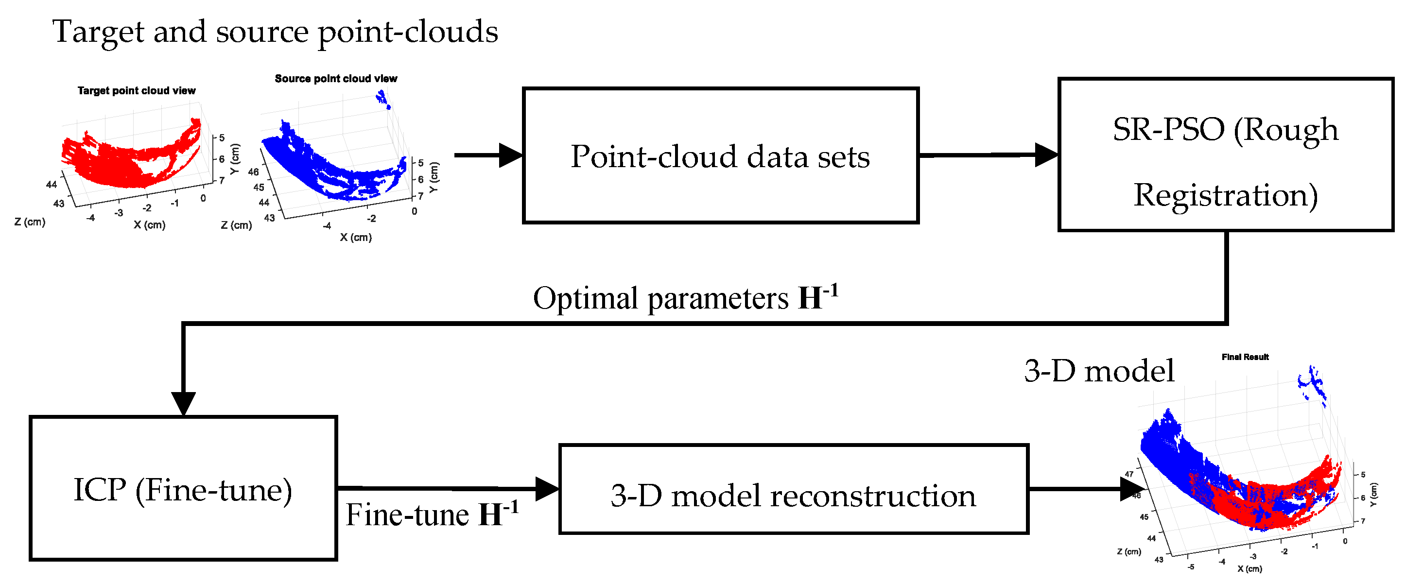
The 3-D tooth model reconstruction system is shown in
Figure 1. The SR-PSO algorithm is used to find the optimal transformation matrix
H−1 (transform from source point-cloud to target point-cloud). The ICP method is used to fine-tune the resultant
H−1. Finally, the 3-D tooth models are reconstructed based on the registered source and target point-clouds.
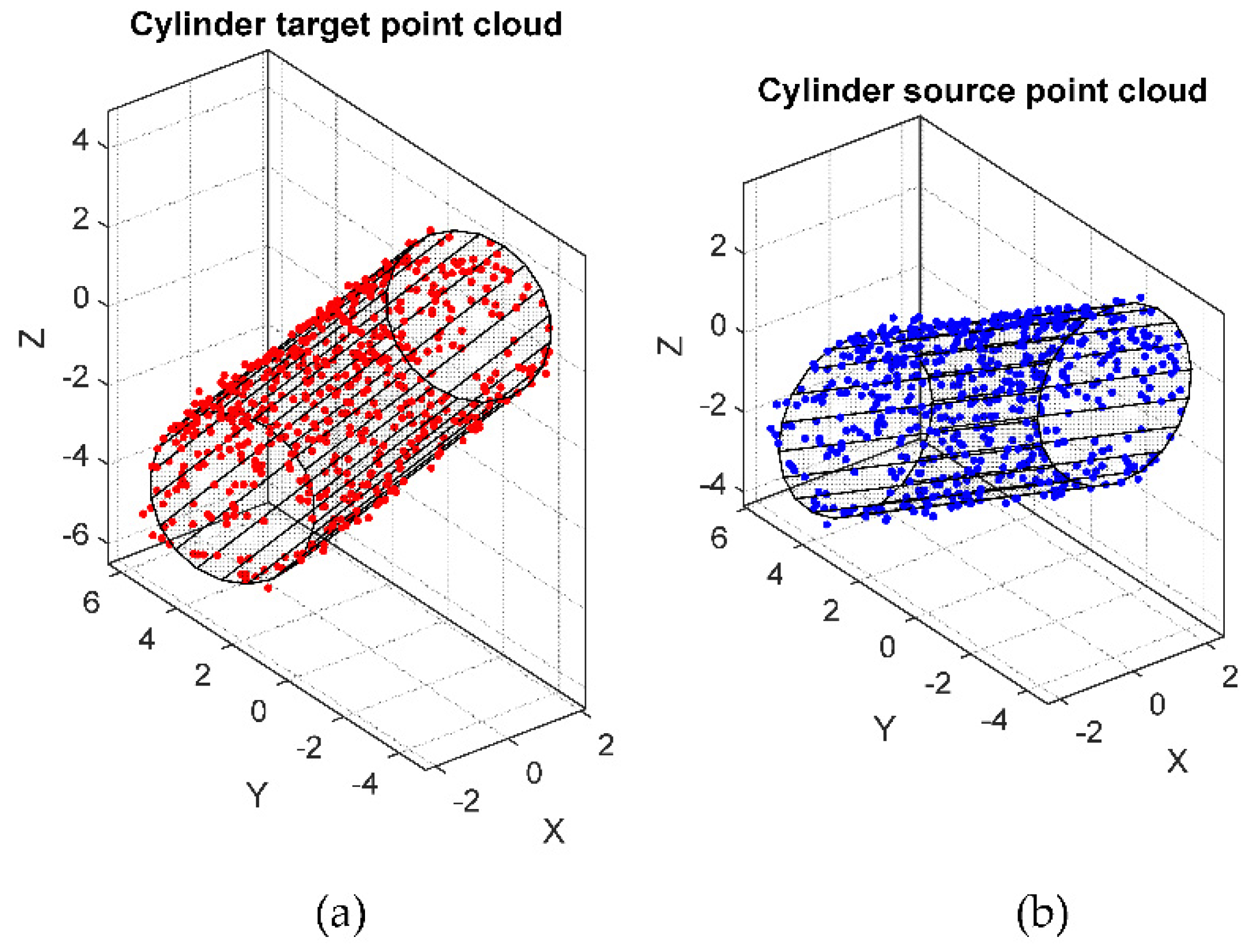
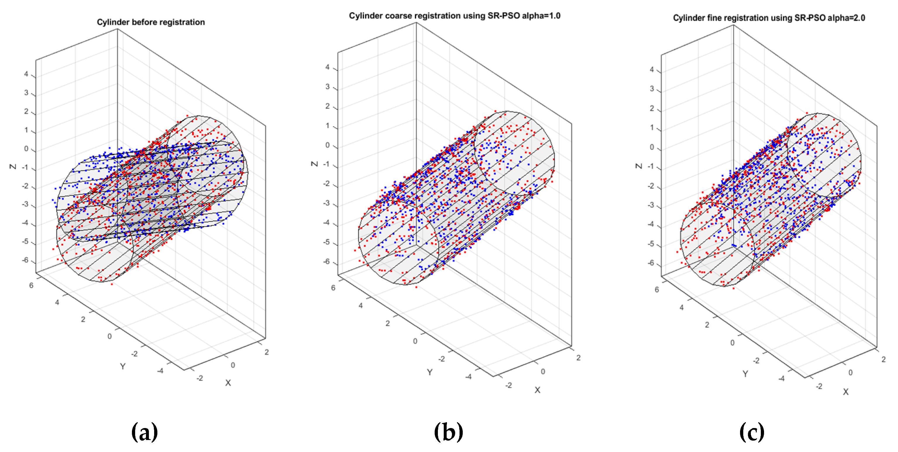
To test the algorithm, we ran the experiment of the generated original shape and its 3-D transformation as shown in
Figure 2.
The transformation matrix used to transform the original shape described by the target point-cloud (
Figure 2a) to the transformed shape described by the source point-cloud (
Figure 2b) is
Hence, the transform matrix from the source point-cloud (
Figure 2b) to the target point-cloud (
Figure 2a) is
In the experiment, the parameters for the SR-PSO algorithm were set as shown in
Table 2. To demonstrate how the SR-PSO algorithm works in each step, we provide an example as follows:
Suppose an initialized particle is , then after the velocity and position are updated, the transformation is . The individual best of this particle is and the global best in this iteration is . Then, all five intermediate particles are ,
,
,
, and
. The best of intermediate particles is
and it is better than
, hence
. Then
from Equation (20) is
. After comparing
with
,
is better, hence
.
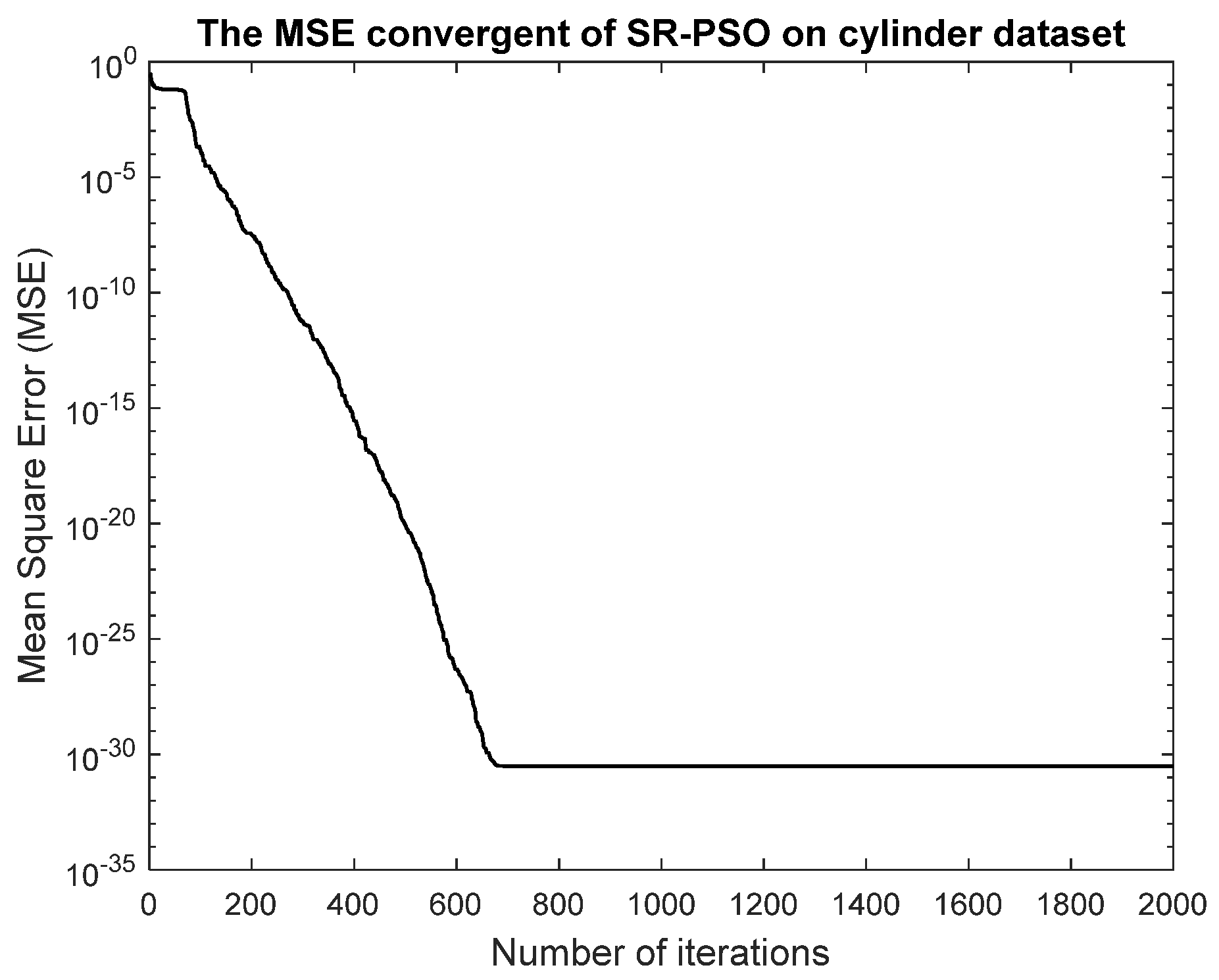
Figure 3 depicts the registration mean-squared error (MSE) of the global best of the SR-PSO algorithm. We can see that, as the iteration proceeds, the MSE decreases and moves towards 3.22 × 10
−31 at the 2000th iteration.
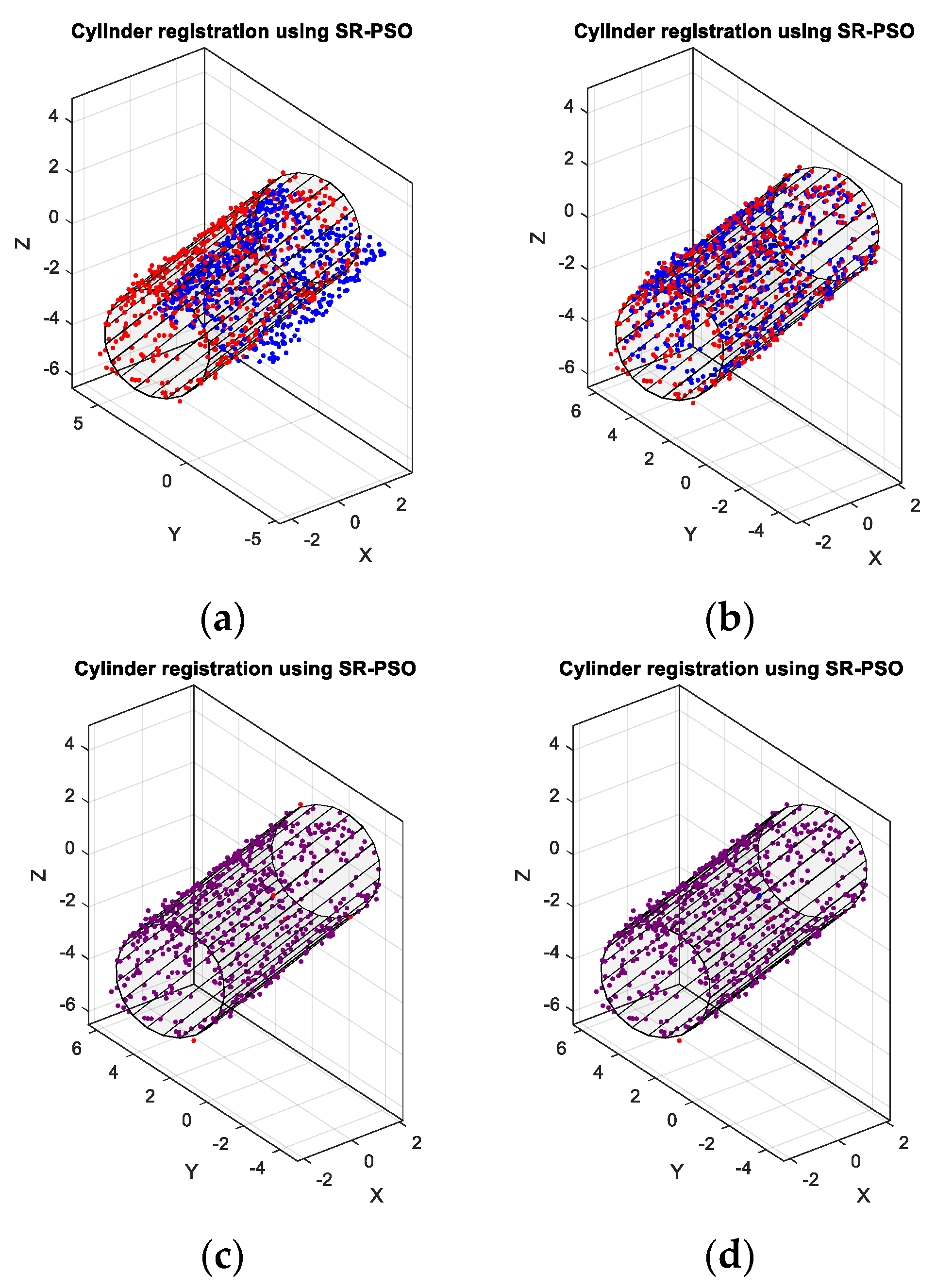
Figure 4 shows the registration progress image of the global best particle in the 1st, 50th, 500th, and 2000th iterations. It can be seen that the registration result in the last iteration is an almost perfect match.
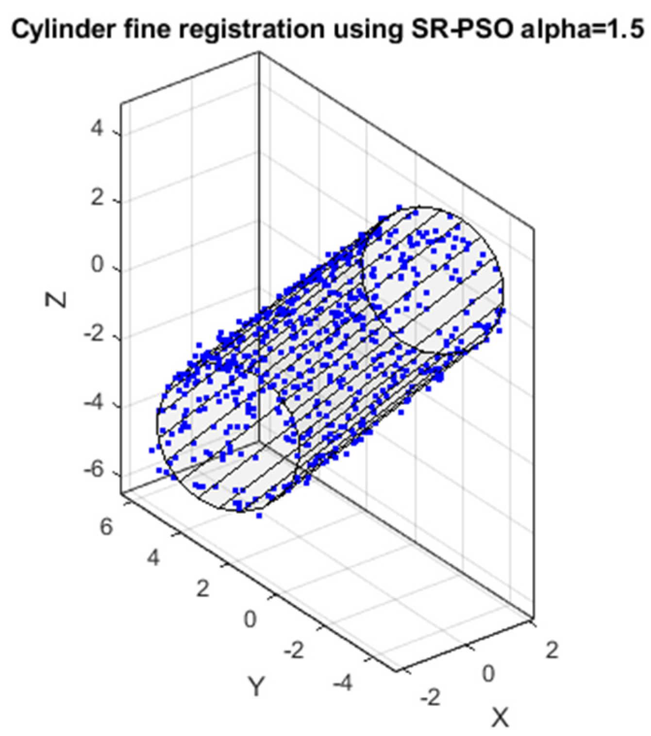
The registration mean-squared errors (MSEs) using the SR-PSO algorithm with and without refining with the ICP method are shown in
Table 3. The best result is when
α = 1.5 with an extremely tiny error of 3.22 × 10
−31. The best final registration result is also shown in
Figure 5.
The best final transformation matrix is
Although the MSEs of the final registration with the other values of
α are not as good, the final registration images are almost aligned as shown in
Figure 6. The reason for this mistake might be because the SR-PSO algorithm does not find the correct global minimum.
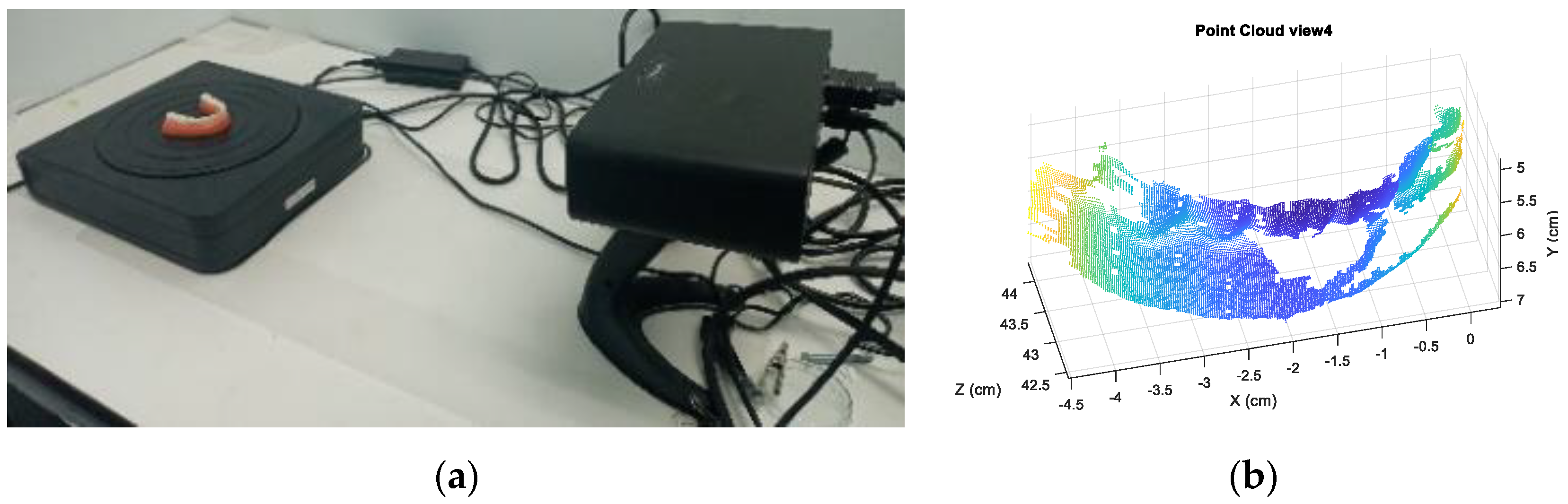
Now, we are ready to implement this algorithm on tooth reconstruction. We used the EinScan series, a commercial 3-D scanner, to collect a point-cloud data set in several consecutive views from two commercial tooth models. Examples of data acquisition setup and the point-cloud data are shown in
Figure 7.
We implemented this system on two different tooth models, i.e., a regular tooth model and an orthodontic tooth model. We used only six consecutive point-cloud coordinate (
x,
y,
z) views with an interval of 30 degrees in each model. The information of the tooth point-cloud data is shown in
Table 4.
In this dataset, we randomly sampled each view into 60% of the original view. We also assumed that there was overlapping between each consecutive view. We also selected representative points inside the overlapping area using the voxel hull method [
33,
34,
35] before we implemented the registration process with the parameter setting shown in
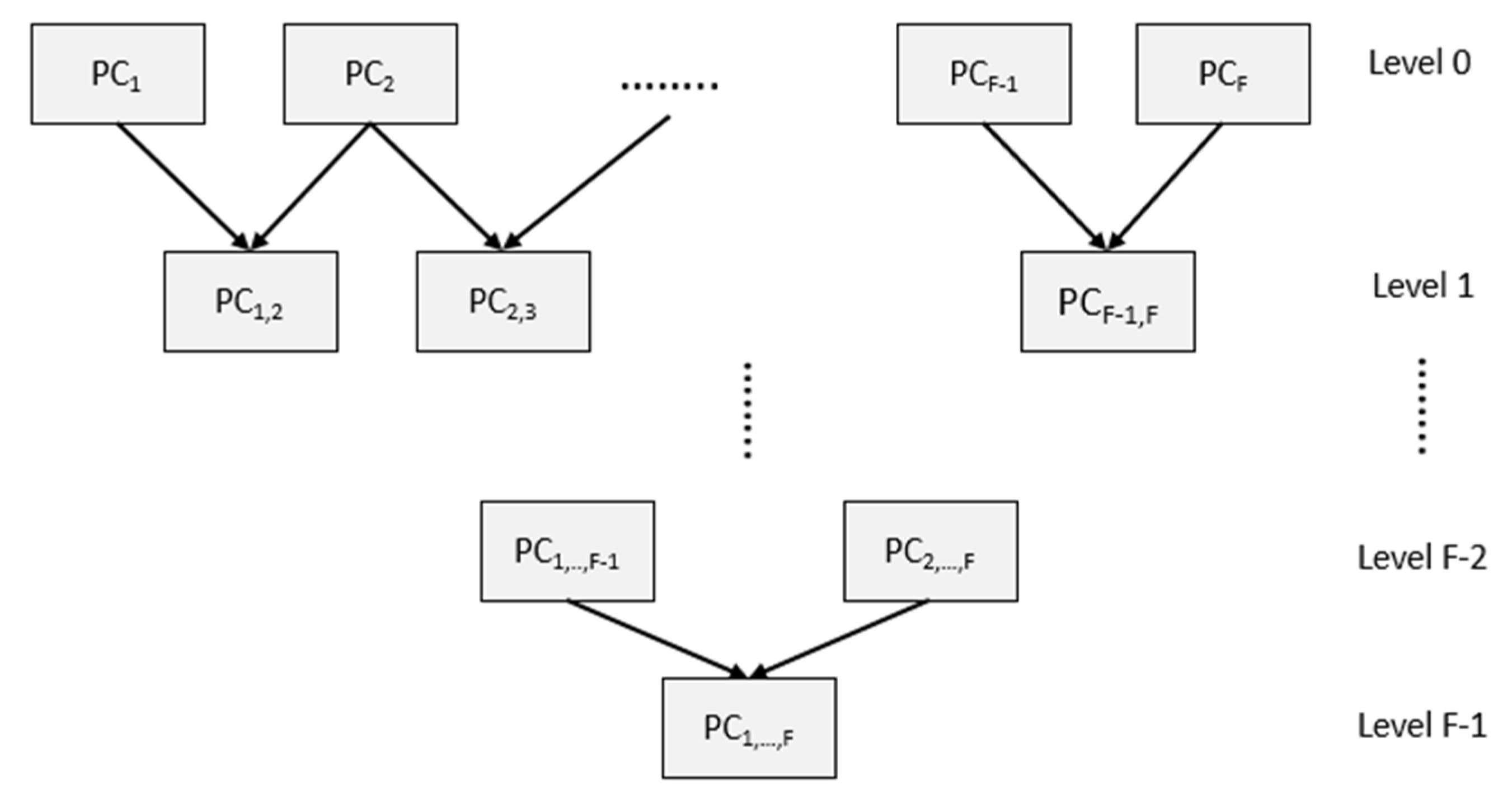
Table 2. Since there were six consecutive views, we utilized the hierarchical registration to increase the registration performance as shown in
Figure 8 with
F = 6. At each level, we selected the best final registration result (SR-PSO algorithm with the ICP method) to survive to the next level of the hierarchical registration.
We also compared the results with those from the regular particle swarm optimization (PSO) algorithm with the ICP method. The registration process from the PSO algorithm with the ICP method is the same as the SR-PSO algorithm with the ICP method. However, the inertia weight update equation in PSO [
29] is
The parameter setting was similar to those used in the SR-PSO algorithm except that wmin, wmax, c1, and c2 were set to 0.4, 0.9, 2, and 2, respectively.
For the regular-tooth model, the registration MSEs for the SR-PSO algorithm and the PSO algorithm for each registration pair are shown in
Table 5. Meanwhile, the registration MSEs for each of the two algorithms with the ICP method for each registration pair are shown in
Table 6.
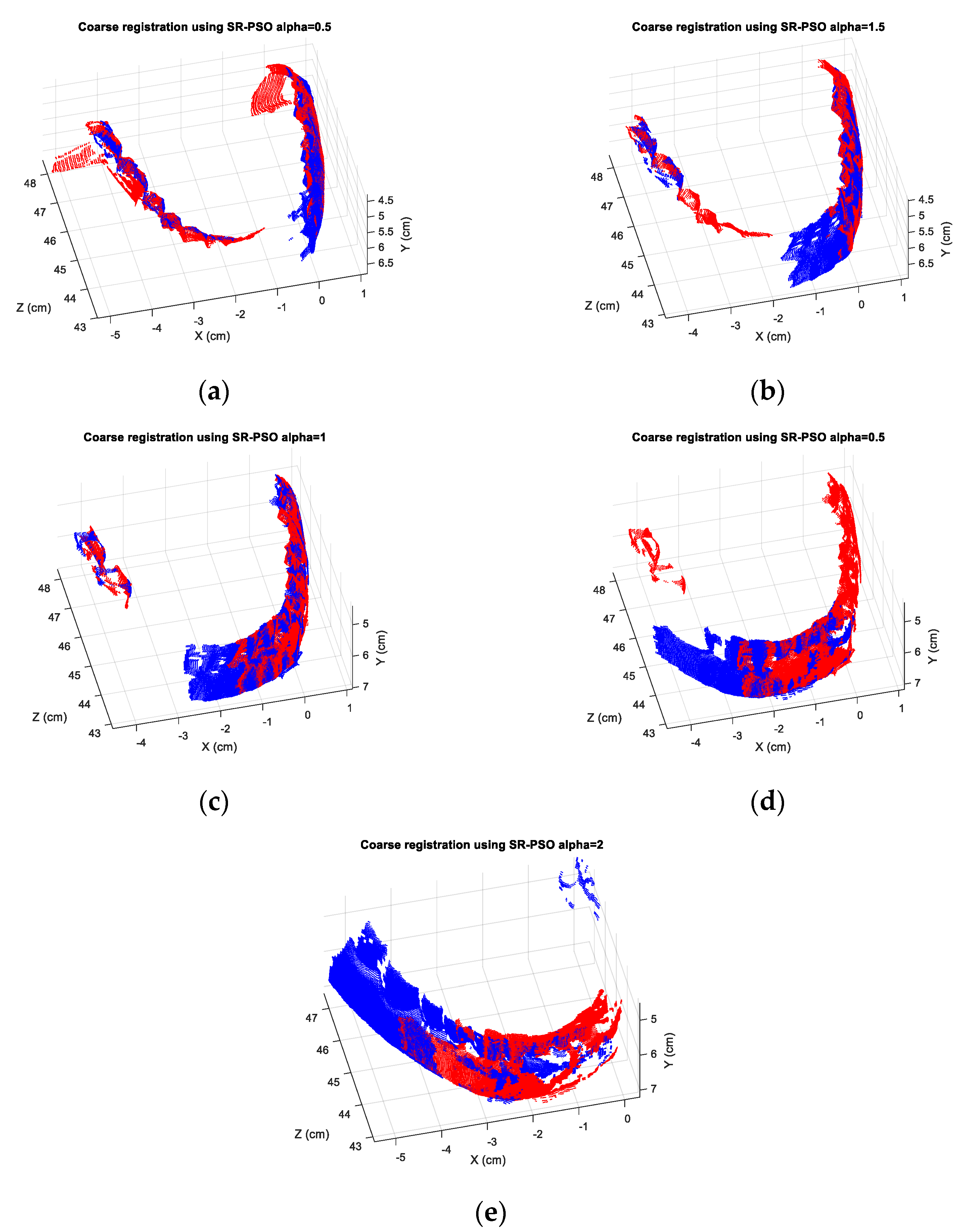
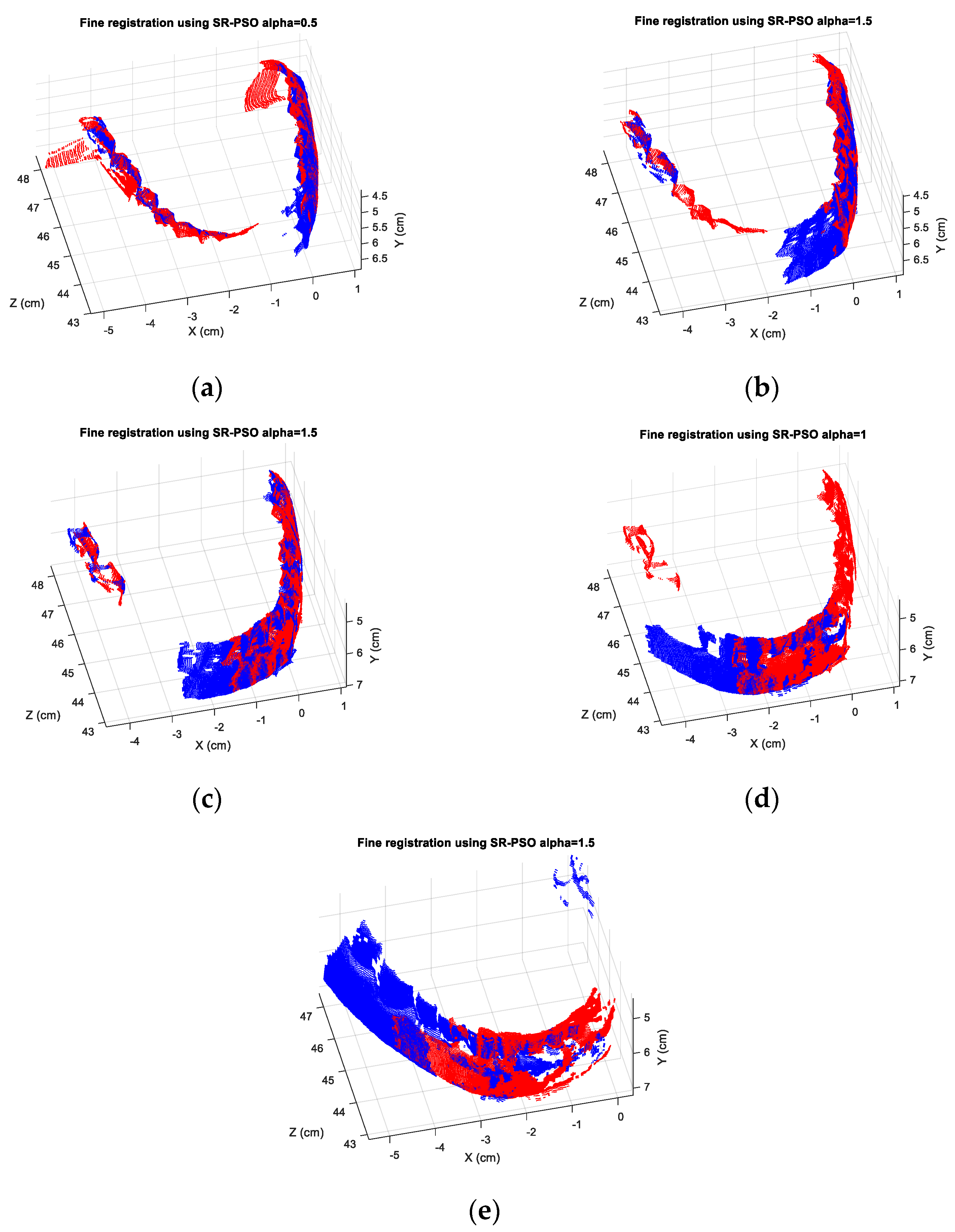
Figure 9 and
Figure 10 show the best registration image of each consecutive pair from the SR-PSO algorithm without and with the ICP method, respectively. Again, the local optima are the cause of high MSE in pair-wise registration. Although
Table 6 shows that the PSO algorithm with the ICP method is a little bit better than the SR-PSO algorithm with the ICP method in some pair-wise registrations, i.e., 1 vs. 2, 2 vs. 3, and 3 vs. 4, the difference is only in the order of 0.002 to 0.05 micrometer
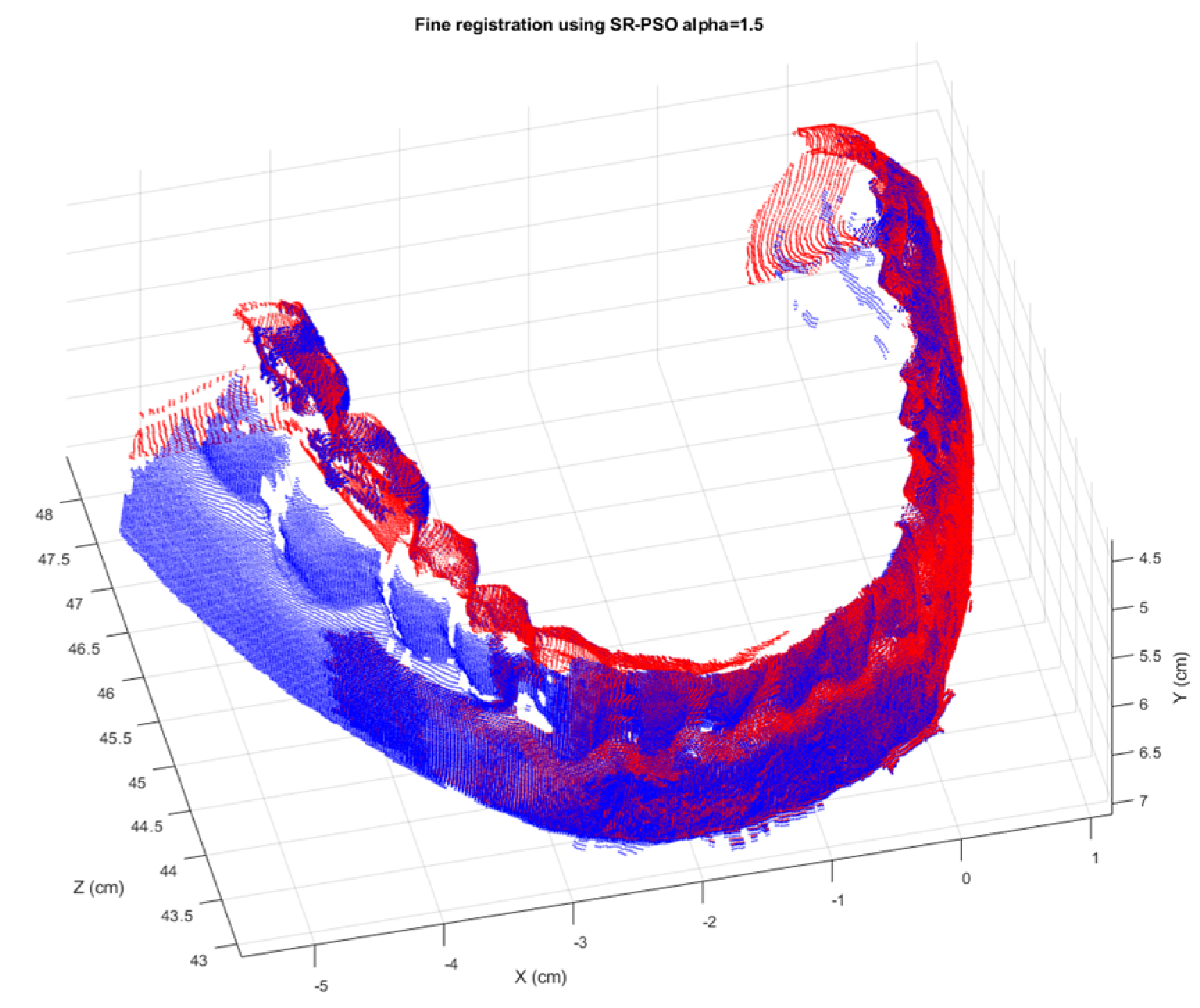
2. When considering the final registration results of six consecutive views shown in
Table 7, we find that the best result from the SR-PSO algorithm with the ICP method and
α = 1.5 is 7.3666 micrometer
2 whereas that from the PSO algorithm with the ICP method is 17.1150 micrometer
2. The result from the SR-PSO algorithm with the ICP method is better than that from the PSO algorithm with the ICP method. The final registration result of the regular-tooth model is shown in
Figure 11. We can see that the final registration image provides a good visualization to human eyes.
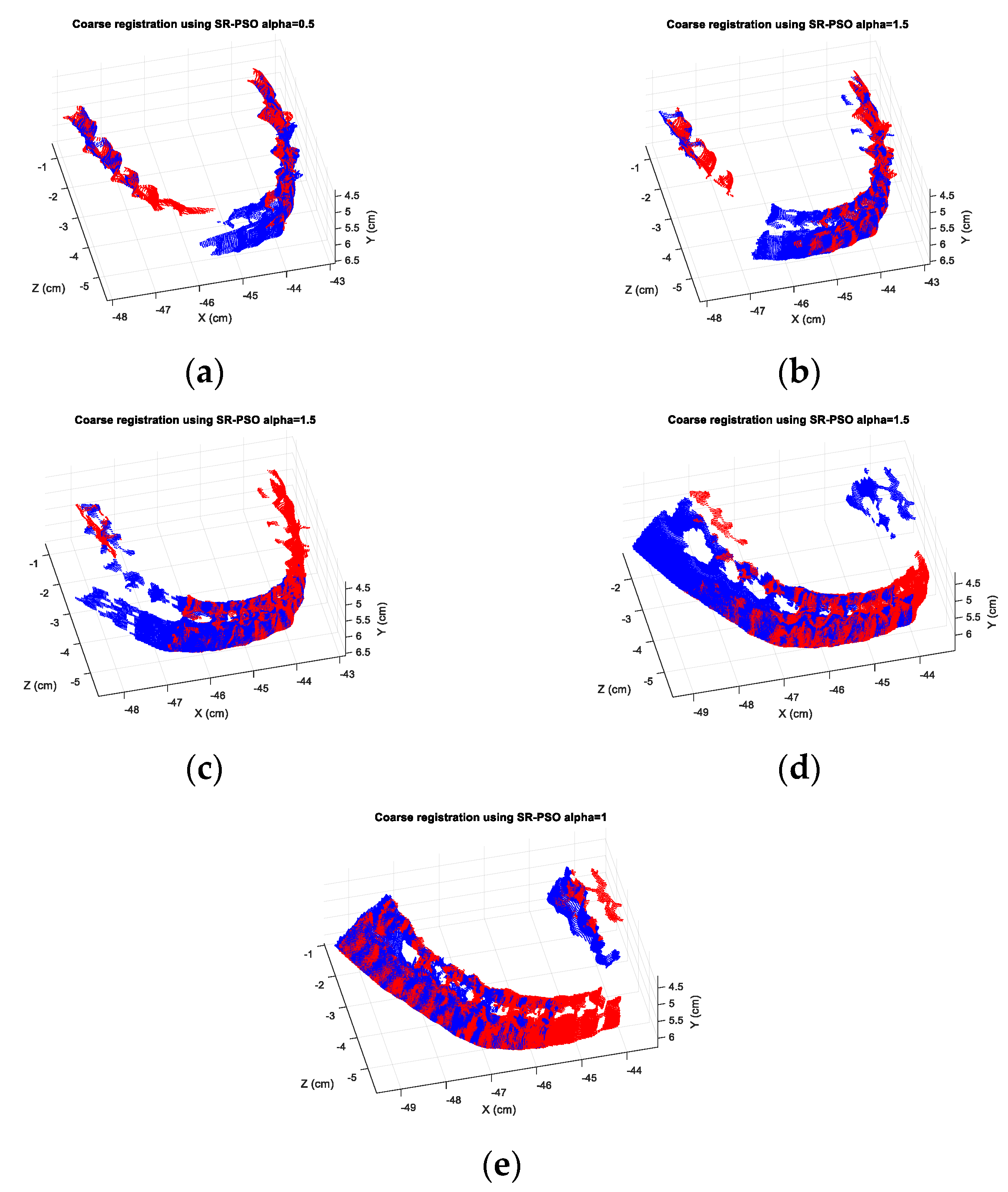
For the orthodontic-tooth model, the registration MSEs for the SR-PSO algorithm and the PSO algorithm for each registration pair are shown in
Table 8.
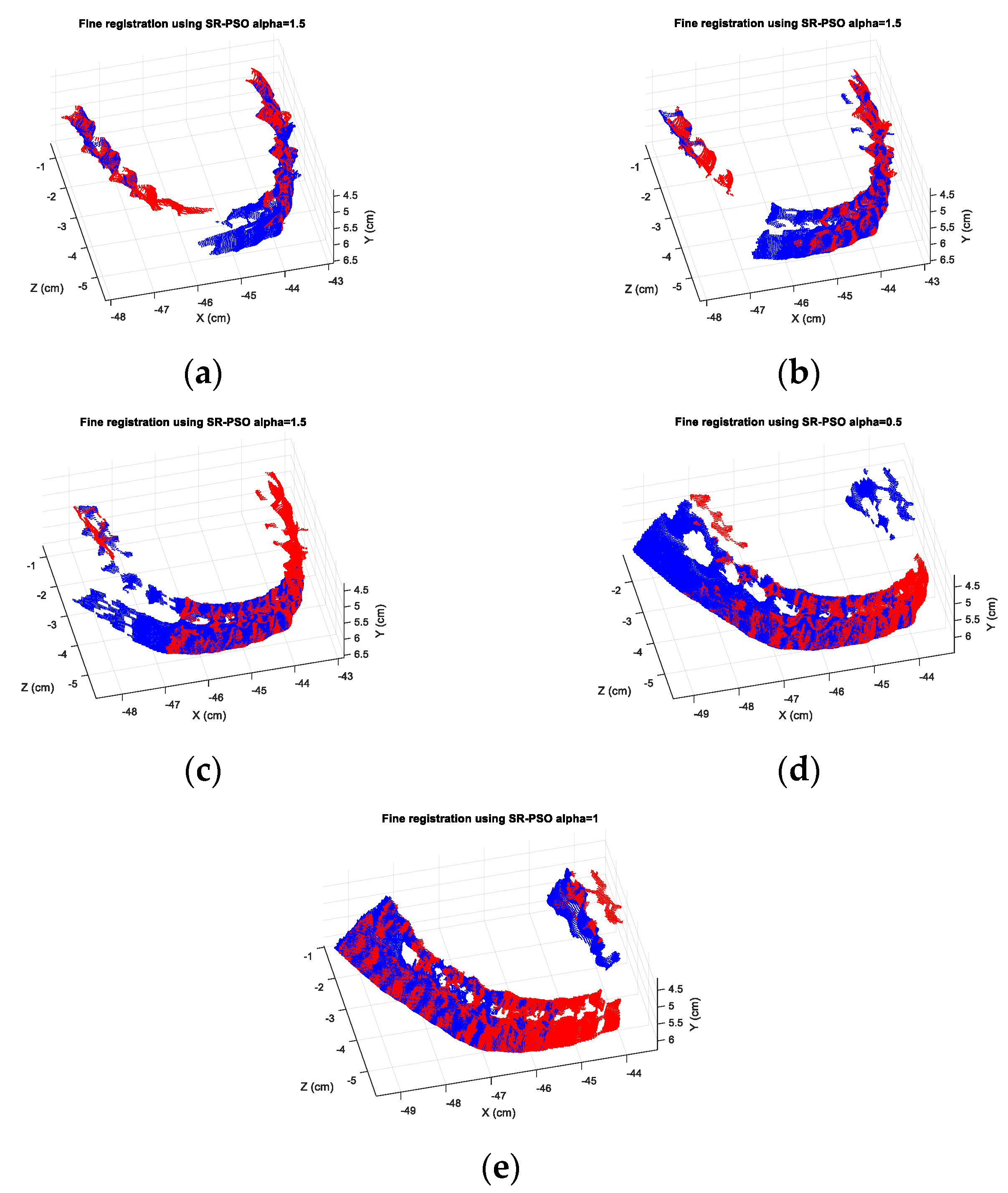
Figure 12 shows the best registration images of different pairs from the SR-PSO algorithm. Meanwhile, the registration MSEs for the SR-PSO algorithm with the ICP method and the PSO algorithm with the ICP method for each registration pair are shown in
Table 9. The best registration images of different pairs from the SR-PSO algorithm with the ICP method are shown in
Figure 13. We can see that using only the SR-PSO algorithm provides better results than using only the PSO algorithm. However, the PSO algorithm with the ICP method is better than the SR-PSO algorithm with the ICP method in one of the pair-wise registrations (4 vs. 5) with a little difference. The final registration MSEs of the six consecutive views are shown in
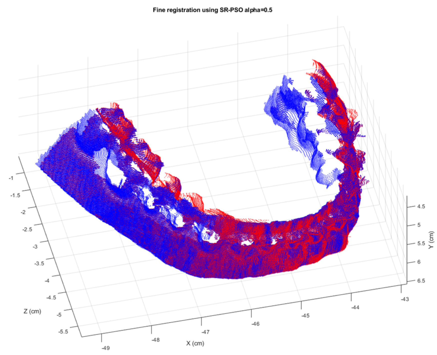
Table 10. The best final 3-D registration image is from the SR-PSO algorithm with the ICP method and
α = 0.5. It has an MSE of 7.4130 micrometer
2 whereas the comparable error of 7.4672 micrometer
2 is achieved by the PSO algorithm with the ICP method. We can also see in
Figure 14 that the final 3-D registration image of the orthodontic-tooth model also provides a good visualization to human eyes.


 ,
, 


