Analytical Solutions of Model Problems for Large-Deformation Micromorphic Approach to Gradient Plasticity

Abstract

The objective of this work is to present analytical solutions for several 2D model problems to demonstrate the unique plastic fields generated by the implementation of micromorphic approach for gradient plasticity. The approach is presented for finite deformations and several macroscopic and nonstandard microscopic boundary conditions are applied to a gliding plate to illustrate the capability to predict the size effects and inhomogeneous plastic fields promoted by the gradient terms. The constitutive behavior of the material undergoing plastic deformation is analyzed for softening, hardening and perfect plastic response and corresponding solutions are provided. The analytical solutions are also shown to match with the numerical results obtained by implementing a user element subroutine (UEL) to the commercial finite element software Abaqus/Standard.

1. Introduction

The size-dependent mechanical behavior of crystalline materials has been clearly shown by various experimental findings in the literature [1,2,3,4,5]. Experiments performed on nano/micro sized metallic specimens (500 nm–50 m) clearly demonstrate the size-dependent nature of their strength which results in inhomogeneous plastic deformation. Lacking an intrinsic length scale, conventional plasticity theories are unable to demonstrate such a size-dependent behavior; therefore, models introducing strain gradient terms in the constitutive relations are widely proposed [6,7,8,9]. Earliest numerical analysis has been performed on theories based on Aifantis yield condition [10,11,12,13]. The Aifantis approach is further developed and established as explicit gradient theories by Peerlings and Geers and the numerical issues have been addressed by the proper regularization of localized deformation with an alternative approach so-called implicit gradient theory [14,15,16].

A significant contribution to introduce a thermodynamically consistent theory for strain gradient plasticity has been done by Gurtin and Anand [17,18,19]. It has been shown that such a thermodynamically consistent theory can also be established by using Eringen’s micromorphic theories of continua [20]. By Eringen’s theory the gradient terms are naturally introduced through higher order degrees of freedom and thermodynamical consistency can be achieved in a systematic fashion by using the principle of virtual power. That track of micromorphic approach is further adopted to several strain gradient problems by Forest and Aslan [21,22,23,24,25] and unified to Gurtin’s thermodynamics [26] by Anand et al. [8].

The micromorphic variable defined as an additional degree of freedom permits the application of unique boundary conditions which brings certain ease to mimic a hard elastic phase, especially for crystalline materials where hardening behavior might strictly depend on geometrically necessary dislocations. Moreover, numerical implementation of such gradient approaches and application of higher order boundary conditions in numerical simulations are very demanding; therefore, reference analytical or semi-analytical solutions are necessary to verify the robustness of the implementation. Even tough, the capability of the micromorphic approach predicting the size effects and inhomogeneous plastic fields promoted by the gradient terms are shown numerically, analytical solutions are provided for only a few model problems in the literature [8,21,22].

The main aim of this paper is to provide analytical solutions for several 2D model problems to demonstrate the unique plastic fields generated by the implementation of micromorphic approach for gradient plasticity. For that purpose, first the approach is presented providing the basic kinematics within the finite strain framework and as an additional degree of freedom to be coupled with the equivalent plastic strain, a microdamage variable $e^p$ is introduced in Section 2. The balance equations are obtained from the principle of virtual power and balance laws are derived. Section 3 presents the micromorphic constitutive equations and provides the general form of analytical solutions for softening and inhomogeneous size-dependent strain hardening. In Section 4, several model problems for a 2d plate under simple shear is scrutinized and the analytical solutions are provided. The analytical results are also shown to match with the numerical results obtained from the implemented user element subroutine (UEL) to the commercial finite element software Abaqus/Standard. The implemented element subroutine is based on a standard four-node isoparametric element on the interpolated fields with $C_0$ continuity. Finally, we close in Section 5 with the final remarks.

2. A Conventional Micromorphic Approach for Gradient Plasticity

2.1. Kinematics

Considering the position of a body denoted by $\mathbf{X}$ in the reference configuration is mapped to the spatial point $\mathbf{x}$ at time t, the motion of that body can be represented by the smooth function $\mathbf{x}=\chi (\mathbf{X},t)$, where velocity, velocity gradient and deformation gradient take the following form:

$$\mathbf{F}=\nabla \chi ,\mathbf{v}=\dot{\chi },\mathbf{L}=\mathrm{grad}\left(\mathbf{v}\right)=\dot{\mathbf{F}}{\mathbf{F}}^{-1},$$

(1)

We consider the multiplicative decomposition of Kröner [27] and the deformation gradient is decomposed into elastic and plastic part

$$\mathbf{F}={\mathbf{F}}^e{\mathbf{F}}^p$$

(2)

where ${\mathbf{F}}^e$ is the elastic distortion which represents the stretch and rotation and ${\mathbf{F}}^p$ represents the local plastic deformation. Please note that ${\mathbf{F}}^p$ is invariant with respect to rigid body motions that are carried by ${\mathbf{F}}^e$. The velocity gradient can be also decomposed into elastic and plastic components in the following form:

$$\mathbf{L}={\mathbf{L}}^e+{\mathbf{F}}^e{\mathbf{L}}^p{{\mathbf{F}}^e}^{-1}$$

(3)

with,

$${\mathbf{L}}^e={\dot{\mathbf{F}}}^e{{\mathbf{F}}^e}^{-1},{\mathbf{L}}^p={\dot{\mathbf{F}}}^p{{\mathbf{F}}^p}^{-1}$$

(4)

The volume ration is expressed as:

$$J=\det \mathbf{F}>0.$$

(5)

Since the plasticity is assumed as incompressible (5), the Jacobian can also be decomposed as

$$J=J^e{J}^p,J^e=\det {\mathbf{F}}^e>0,J^p=\det {\mathbf{F}}^p=1.$$

(6)

The right polar decomposition of ${\mathbf{F}}^e$ yields

$${\mathbf{F}}^e={\mathbf{R}}^e{\mathbf{U}}^e$$

(7)

where ${\mathbf{U}}^e$ is the right stretch tensor and ${\mathbf{R}}^e$ is the rotation tensor. Then, the right elastic Cauchy-Green tensor and the stretch tensor read the following

$${\mathbf{C}}^e={\left({\mathbf{U}}^e\right)}^2={\mathbf{F}}^e{}^T{\mathbf{F}}^e$$

(8)

$${\mathbf{U}}^e=\sum _{i=3}^3{\lambda }_i^e{r}_i^e\otimes r_i^e$$

(9)

As a strain measure, Hencky’s logarithmic strain [28] is chosen due to its good agreement with experiments on a wide class of materials [29,30]

$${\mathbf{E}}^e=\ln \left({\mathbf{U}}^e\right)=\sum _{i=1}^3{E}_i^e{\mathbf{r}}_i^e\otimes {\mathbf{r}}_i^e$$

(10)

The elastic and inelastic stretching and spin tensors are

$${\mathbf{D}}^e=\mathrm{sym}{\mathbf{L}}^e,{\mathbf{D}}^p=\mathrm{sym}{\mathbf{L}}^p$$

(11)

$${\mathbf{W}}^e=\mathrm{skew}{\mathbf{L}}^e,{\mathbf{W}}^p=\mathrm{skew}{\mathbf{L}}^p$$

(12)

Assuming irrotational plastic evolution i.e.,

$${\mathbf{W}}^p=0$$

(13)

the rate of plastic deformation gradient would be

$${\dot{\mathbf{F}}}^p={\mathbf{D}}^p{\mathbf{F}}^p,{\mathbf{F}}^p(\mathbf{X},\mathbf{0})=\mathbf{1}$$

(14)

Introducing a positive-valued equivalent tensile stress and corresponding plastic strain rate

$$\overline{\sigma }=\sqrt{3/2}|{\mathbf{M}}_0^{\mathbf{e}}|\mathrm{and}{\dot{\overline{ϵ}}}^p\sqrt{2/3}\left|{\mathbf{D}}^{\mathbf{p}}\right|$$

(15)

where ${\mathbf{M}}_0^{\mathbf{e}}$ is the deviatoric component of the Mandel stress and the direction of the plastic flow becomes

$${\mathbf{N}}^{\mathbf{p}}=\frac{{\mathbf{M}}_0^{\mathbf{e}}}{|{\mathbf{M}}_0^{\mathbf{e}}|}$$

(16)

2.2. Micromorphic Variable $e^p$

The micromorphic counterpart for the equivalent plastic strain, ${\overline{ϵ}}^p$ is defined as ${\mathrm{e}}^{\mathrm{p}}$ for the sake of mathematical regularization as an additional kinematical degree of freedom [8]. Please note that ${\mathrm{e}}^{\mathrm{p}}$ is a frame-indifferent, positive scalar microvariable which constitutes a subset of micromorphic continuum. The calculation of its gradient $\nabla {\mathrm{e}}^{\mathrm{p}}$ numerically comes at ease, since ${\mathrm{e}}^{\mathrm{p}}$ is defined as an extra degree of freedom. Considering the principle of virtual power, the power over ${\dot{\overline{ϵ}}}^p$ is expended by the equivalent stress $\overline{\sigma }$, ${\dot{\mathrm{e}}}^{\mathrm{p}}$ is expended by the scalar microscopic stress $\mathbf{p}$, $\nabla {\dot{\mathrm{e}}}^{\mathrm{p}}$ is expended by the microscopic stress vector $\xi$, and ${\dot{\mathrm{e}}}^{\mathrm{p}}$ is expended by the microscopic traction $\zeta \left({\mathbf{n}}_{\mathrm{R}}\right)$ at the boundary.

2.3. Balance Equations

The proposed theory restricts the gradient effect to a scalar variable ${\overline{ϵ}}^p$ which results in only one additional degrees of freedom providing significant efficiency in computations. Therefore, degrees of freedoms are the displacement vector $u_i$ and the scalar microvariable ${\mathrm{e}}^{\mathrm{p}}$. The degrees of freedom and their gradient in the form of strain-like variables are as follows:

$$DOF=\{u_i,{\mathrm{e}}^{\mathrm{p}}\}STRAIN=\{{\mathbf{E}}^{\mathbf{e}},{\overline{ϵ}}^p,{\mathrm{e}}^{\mathrm{p}},\nabla {\mathrm{e}}^{\mathrm{p}}\}$$

(17)

Considering the definitions provided in Section 2.2, the variation of any independent variable in the system will cause an energy change and neglecting the kinetic energy, external and internal expenditures of virtual power for any given part P are defined as follows

$$\begin{array}{cc}\hfill W_{ext}& ={\int }_{\partial P}({\mathbf{t}}_{\mathrm{R}}\left({\mathbf{n}}_{\mathrm{R}}\right)·\dot{\chi }dS+{\int }_P{\mathbf{b}}_{\mathrm{R}}·\dot{\chi }dV+{\int }_{\partial P}\zeta \left({\mathbf{n}}_{\mathrm{R}}\right){\dot{\mathrm{e}}}^{\mathrm{p}}\mathrm{dS}\hfill \\ \hfill W_{int}& ={\int }_P({\mathbf{S}}_R:{\dot{\mathbf{F}}}^e+\overline{\sigma }{\dot{\overline{ϵ}}}^p+\mathbf{p}{\dot{\mathrm{e}}}^{\mathrm{p}}+\xi ·\nabla {\dot{\mathrm{e}}}^{\mathrm{p}})\mathrm{dV}\hfill \end{array}$$

(18)

accordingly, the 1st Piola–Kirchhoff stress tensor, ${\mathbf{T}}_{\mathrm{R}}$ is defined as

$${\mathbf{T}}_{\mathrm{R}}={\mathbf{S}}_{\mathrm{R}}{\mathbf{F}}^{p-T}$$

(19)

Principle of virtual power dictates that for any given part P and for all generalized virtual rates the external and internal powers are balanced:

$$W_{ext}=W_{int}$$

(20)

considering ${\dot{\overline{ϵ}}}^p\equiv 0$ and ${\dot{\mathrm{e}}}^{\mathrm{p}}\equiv 0$ and applying divergence theorem, the macroscopic force balance and the traction condition become

$$\mathrm{Div}{\mathbf{T}}_{\mathrm{R}}+{\mathbf{b}}_{\mathrm{R}}=\mathbf{0}$$

(21)

$${\mathbf{t}}_{\mathrm{R}}\left({\mathbf{n}}_{\mathrm{R}}\right)={\mathbf{T}}_{\mathrm{R}}{\mathbf{n}}_{\mathrm{R}}$$

(22)

Considering $\dot{\chi }\equiv 0$ and ${\dot{\overline{ϵ}}}^p\equiv 0$, choosing an arbitrary ${\dot{\mathrm{e}}}^{\mathrm{p}}$ field and applying divergence theorem, the microscopic force balance and the traction condition become

$$\mathrm{Div}\xi -\mathbf{p}=0$$

(23)

$$\zeta \left({\mathbf{n}}_{\mathrm{R}}\right)=\xi ·{\mathbf{n}}_{\mathrm{R}}$$

(24)

3. Constitutive Equations

Before the presentation of the constitutive equations, several stress measures need to be introduced to be used in the model.

The Mandel stress is defined by

$${\mathbf{M}}^e={\mathbf{C}}^e{\mathbf{T}}^e$$

(25)

The second Piola stress can be calculated from the Mandel stress such as

$${\mathbf{T}}^e={{\mathbf{F}}^e}^{-1}{{\mathbf{F}}^e}^{-T}{\mathbf{M}}^e$$

(26)

In connection with Equation (25), the Cauchy stress can be computed using the equation below.

$$\mathbf{T}=J^{-1}{\mathbf{F}}^e{\mathbf{M}}^e{{\mathbf{F}}^e}^T$$

(27)

Finally, the first Piola stress becomes

$${\mathbf{T}}_R=J\mathbf{T}{\mathbf{F}}^{-T}$$

(28)

For the given model, the free energy is considered to be a quadratic potential as a function of elastic strain, ${\mathbf{E}}^e$, equivalent plastic strain, ${\overline{ϵ}}^p$, microvariable, ${\dot{\mathrm{e}}}^{\mathrm{p}}$ and its gradient, $\nabla {\dot{\mathrm{e}}}^{\mathrm{p}}$. The coupling is introduced between the scalar microvariable, ${\dot{\mathrm{e}}}^{\mathrm{p}}$ and its macroscopic counterpart, equivalent plastic strain, ${\overline{ϵ}}^p$ in the form of an energetic penalty term.

$$\psi =\widehat{\psi }({\mathbf{E}}^e,{\overline{ϵ}}^p,{\dot{\mathrm{e}}}^{\mathrm{p}},\nabla {\dot{\mathrm{e}}}^{\mathrm{p}})=\mu |{\mathbf{E}}^e{|}^2+\frac{1}{2}\lambda {\left(tr{\mathbf{E}}^e\right)}^2+\frac{1}{2}B{({\overline{ϵ}}^p-{\dot{\mathrm{e}}}^{\mathrm{p}})}^2+\frac{1}{2}\beta {|\nabla {\dot{\mathrm{e}}}^{\mathrm{p}}|}^2$$

(29)

where $\mu ,\kappa ,B$ and $\beta$ are positive material constants and the energetic state relations are derived from the normality:

$${\mathbf{T}}^e=\frac{\partial \widehat{\psi }({\mathbf{E}}^e,{\overline{ϵ}}^p,{\dot{\mathrm{e}}}^{\mathrm{p}},\nabla {\dot{\mathrm{e}}}^{\mathrm{p}})}{\partial {\mathbf{E}}^e}$$

(30)

$$\overline{\sigma }=\frac{\partial \widehat{\psi }({\mathbf{E}}^e,{\overline{ϵ}}^p,{\dot{\mathrm{e}}}^{\mathrm{p}},\nabla {\dot{\mathrm{e}}}^{\mathrm{p}})}{\partial {\overline{ϵ}}^p}$$

(31)

$$p=\frac{\partial \widehat{\psi }({\mathbf{E}}^e,{\overline{ϵ}}^p,{\dot{\mathrm{e}}}^{\mathrm{p}},\nabla {\dot{\mathrm{e}}}^{\mathrm{p}})}{\partial {\mathrm{e}}^{\mathrm{p}}}$$

(32)

$$\xi =\frac{\partial \widehat{\psi }({\mathbf{E}}^e,{\overline{ϵ}}^p,{\dot{\mathrm{e}}}^{\mathrm{p}},\nabla {\dot{\mathrm{e}}}^{\mathrm{p}})}{\partial \nabla {\mathrm{e}}^{\mathrm{p}}}$$

(33)

$$\begin{array}{cc}\hfill \overline{\sigma }& =B{({\overline{ϵ}}^p-{\mathrm{e}}^{\mathrm{p}})}^2\hfill \\ \hfill \mathbf{p}& =-B{({\overline{ϵ}}^p-{\mathrm{e}}^{\mathrm{p}})}^2\hfill \\ \hfill \xi & =\beta \nabla {\mathrm{e}}^{\mathrm{p}}\hfill \end{array}$$

(34)

Furthermore, recalling Equation (23), the microscopic force balance takes the form of Helmholtz equation which is postulated in the so-called implicit gradient theory of plasticity and damage [14,15,16], where the microvariables are called non-local variables and where the generalized stresses $\mathbf{p}$ and $\xi$ are not explicitly introduced.

$$\mathrm{Div}\xi =\beta \Delta {\mathrm{e}}^{\mathrm{p}}$$

(35)

which is a form of Helmholtz equation:

$${\mathrm{e}}^{\mathrm{p}}-\frac{\beta }{B}\Delta {\mathrm{e}}^{\mathrm{p}}={\overline{ϵ}}^p$$

(36)

$$\beta \Delta e^p+B({\overline{ϵ}}^p-{\mathrm{e}}^{\mathrm{p}})=0$$

(37)

A yield criterion can be defined as

$$f=\overline{\sigma }-Y({\overline{ϵ}}^p,{\mathrm{e}}^{\mathrm{p}})=0$$

(38)

where the microscopic stress becomes

$$\overline{\sigma }=Y({\overline{ϵ}}^p,{\mathrm{e}}^{\mathrm{p}})$$

(39)

Considering a rate independent plastic evolution with linear isotropic hardening/softening, a microforce balance with the gradient enhancement can be considered such as

$$\overline{\sigma }=S_a+H{\overline{ϵ}}^p+B({\overline{ϵ}}^p-{\mathrm{e}}^{\mathrm{p}})$$

(40)

In the scope of this work, $\overline{\sigma }$ is equivalent tensile stress, $S_a$ is the initial yield strength and H is the hardening/softening modulus. Further using (37), one can write (40) as:

$$\overline{\sigma }=S_a+H{\mathrm{e}}^{\mathrm{p}}+\frac{(H+B)\beta }{B}\Delta {\mathrm{e}}^{\mathrm{p}}$$

(41)

solving (41) for ${\mathrm{e}}^{\mathrm{p}}$ gives:

$${\mathrm{e}}^{\mathrm{p}}=\frac{\overline{\sigma }-S_a}{H}+\frac{(H+B)\beta }{B}\Delta {\mathrm{e}}^{\mathrm{p}}$$

(42)

Please note that (42) is a second order homogeneous differential equation with the following general form:

$$y^{″}-\omega y=C$$

(43)

where

$$\omega =\sqrt{\frac{HB}{\beta (B+H)}}\mathrm{and}C=\frac{\overline{\sigma }-S_a}{H}$$

(44)

which has two different solutions depending on the sign of $\omega$

$$Asinh\left(x\sqrt{\omega }\right)+Bcosh\left(x\sqrt{\omega }\right)+Cif\omega >0$$

(45)

$$Asin\left(x\sqrt{\omega }\right)+Bcos\left(x\sqrt{\omega }\right)+Cif\omega <0$$

(46)

For a softening material, where $\omega <0$ and $H<0$, the wave period of the sine function provides the width of the localization band, which reads

$$\frac{2\pi }{\omega }=2\pi \sqrt{\frac{\beta (B+H)}{HB}}$$

(47)

4. Model Problems

4.1. Simple Glide of a Softening Plate with a Central Imperfection

As a model problem, simple glide of an infinite plate with an initial height of h is considered (Figure 1). The plate is assumed to behave plastically with linear softening and an infinitely long imperfection is placed at the center to trigger localization. For the finite element analysis, a finite plate is analyzed with proper periodic conditions.

Figure 1. Schematic of the simple glide problem for softening: periodic conditions are applied at both ends.

From the general solution given in (46), a specific solution can be attained at $x_2=h/2$, where it takes the form:

$$\frac{\overline{\sigma }-S_a}{H}\left[cos(w(x_2-h/2)+1\right]$$

(48)

The comparison between the analytical solution and the numerical result is shown in Figure 2 for a given h.

Figure 2. Comparison between numerical and analytical solution for the softening plate. Parameters: B = 10.0 GPa, $\beta$ = 500.0 MPa mm${}^2$, H = −500.0 MPa, h = 10 mm.

4.2. Simple Glide of a Perfectly Plastic Plate with Hard Boundary Conditions

To achieve perfect plastic response hardening modulus is considered to be $H=0.0$ and a plate under simple glide is analyzed in this section. The boundary conditions specified in Figure 3 are applied. Please note that for this special condition (41) becomes:

$$\overline{\sigma }=S_a-\beta \Delta {\mathrm{e}}^{\mathrm{p}}$$

(49)

which is a second order homogeneous differential equation with a general form:

$$y^{″}=C$$

(50)

and general solution becomes:

$$A{x}^2+Bx+C$$

(51)

where

$$C=\frac{Sa-\overline{\sigma }}{2\beta }$$

(52)

finally, considering hard boundary conditions ${\mathrm{e}}^{\mathrm{p}}(x_1,0)=0,{\mathrm{e}}^{\mathrm{p}}(x_1,h)=0$, the solution can be rewritten for the model problem as:

$$\frac{Sa-\overline{\sigma }}{2\beta }(x_2^2-h{x}_2)$$

(53)

Figure 3. Schematic of the simple glide problem for hardening and perfectly plastic plate: periodic conditions are applied at both ends.

The solution given in (53) is in quadratic form and as shown in Figure 4, the plastic strain profile essentially does not provide a boundary layer, even for various intrinsic length scales. The outcome of this boundary value problem is well in line with the findings of Anand et al. [18] where formation of boundary layer is only possible with internal variable hardening. The numerical results are also shown to provide a perfect match with the calculated analytical response.

Figure 4. Comparison between numerical and analytical solution for perfect plastic plate. Parameters: B = 10.0 GPa, $\beta$ = 300, 500, 2000, 1 $\times {10}^4$, 1 $\times {10}^5$, 1 $\times {10}^6$, 1 $\times {10}^7$ MPa mm${}^2$, H = 0.0 MPa, h = 10 mm. To prevent crowding, analytical curves are only provided for $\beta =300$ and $\beta =1\times {10}^6$.

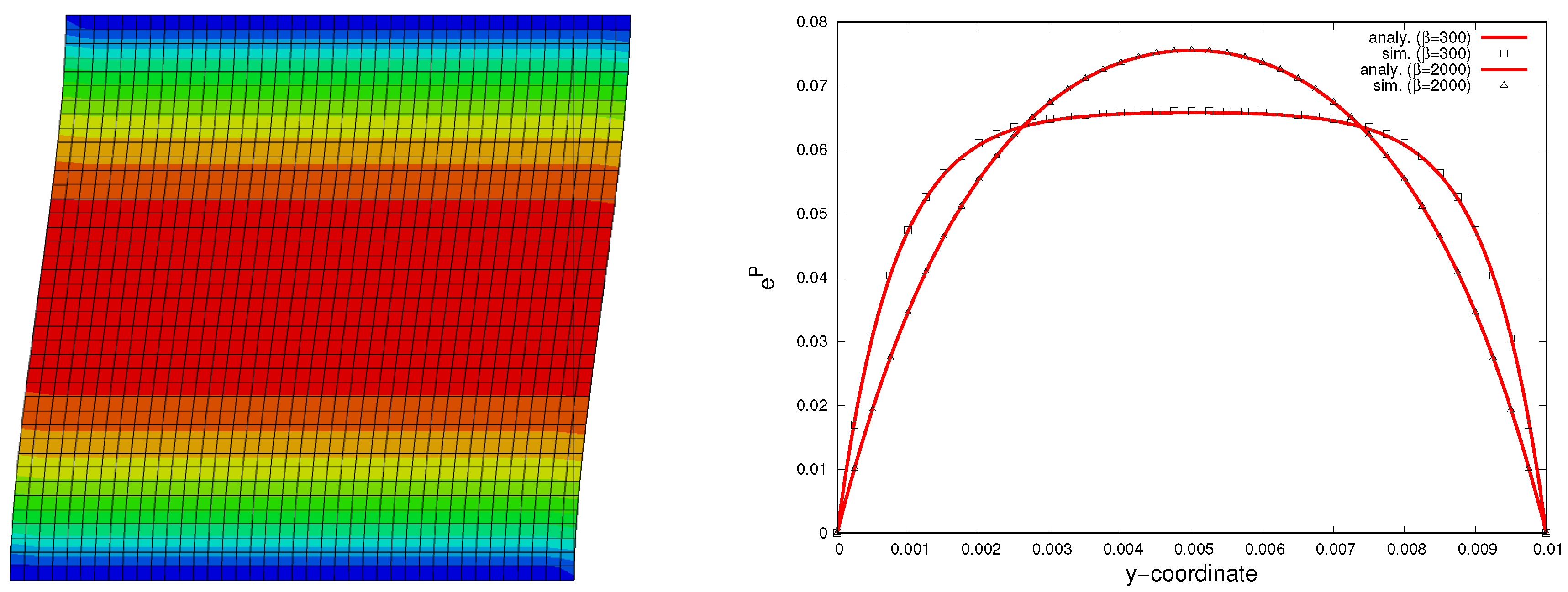
4.3. Simple Glide of a Hardening Plate with Hard Boundary Conditions

As a hardening case, simple glide of an infinite plate with an initial height of h is considered with the same hard boundary conditions specified in Figure 3. The plate is assumed to behave plastically with linear hardening and the hard boundary conditions ${\mathrm{e}}^{\mathrm{p}}(x_1,0)=0,{\mathrm{e}}^{\mathrm{p}}(x_1,h)=0$ are applied (Figure 3).

Considering the first boundary condition ${\mathrm{e}}^{\mathrm{p}}(x_1,0)=0$, the general solution (45) takes the form:

$$B+C=0,withC=\frac{\overline{\sigma }-S_a}{H}$$

(54)

and trivially:

$$B=-C$$

(55)

From the second condition ${\mathrm{e}}^{\mathrm{p}}(x_1,h)=0$, (45) reads:

$$Asinh\left(h\omega \right)-Ccosh\left(h\omega \right)+C=0,with\omega =\sqrt{\frac{HB}{\beta (B+H)}}$$

(56)

solving for A gives:

$$A=\frac{C(cosh(h\omega )-1)}{sinh\left(h\omega \right)}$$

(57)

finally, general solutions becomes:

$$C\left[\frac{(cosh(hw)-1)}{sinh\left(hw\right)}sinh\left(\omega x_2\right)-cosh\left(\omega x_2\right)+1\right]$$

(58)

The solution given in (58) has a unique character where the plastic strain profile shows a boundary layer for small values of $\omega$ with sharp strain plastic gradients in the vicinity of $x_2=0$ and $x_2=h$. However, as $\omega \to 1.0$ the profile gains a parabolic character similar to perfect plastic case. Those two different characteristic responses are shown in Figure 5 where two different length scales for $\omega >1.0(\beta =300)$ and $\omega <1.0(\beta =2000)$ are analyzed with proper periodic conditions. The numerical results are shown to provide a perfect match with the calculated analytical response and they both clearly demonstrate the formation of boundary layer for small $\omega$ values.

Figure 5. Comparison between numerical and analytical solution for the hardening plate. Parameters: B = 10.0 GPa, $\beta$ = 300.0 MPa mm${}^2$ and 2000.0 MPa mm${}^2$, H = 500.0 MPa, h = 10 mm.

5. Concluding Remarks

In this work, we have presented analytical and numerical solutions for three different characteristic response (softening, perfect plastic and hardening) for an infinite gliding plate, to demonstrate the unique plastic fields generated by the implementation of micromorphic approach for gradient plasticity.

For the softening case, our analytical effort clearly presents the characteristic solution which controls the size of the localization band where an intrinsic length scale is defined, and our numerical findings also verify the band formation which is controlled by the wavelength of the sinusoidal function.

Considering the perfect plastic response, our findings are well in line with similar approaches in the literature where the profile of the plastic strain parabolic and the formation of boundary layer is not possible without an internal variable hardening.

With hard boundary conditions and considering linear hardening response, our analytical predictions show that the response of the gliding plate is defined by a hyperbolic function with unique properties. The plastic strain profile shows a boundary layer for small values of $\omega$ with sharp strain plastic gradients around top and bottom layer which mimics a hard phase material at the boundaries. It is also observed that the analytical solution yields a parabolic response for $\omega >1.0$ similar to perfect plastic case.

Our study shows that the micromorphic approach for gradient plasticity has a great potential in representing the size-dependent behavior for both softening and hardening response of crystalline solids which also provides unique possibilities to apply higher order boundary conditions. The approach makes it possible to control the size-dependent behavior with a single length scale parameter and our numerical findings are encouraging to use the presented model for more complex 3D problems.

References

1. Stelmashenko, N.A.; Walls, M.G.; Brown, L.M.; Milman, Y.V. Microindentations on W and Mo oriented single crystals: An STM study. Acta Metall. Mater. 1993, 41, 2855–2865. [Google Scholar] [CrossRef]
2. Ma, Q.; Clarke, D.R. Size dependent hardness of silver single crystals. J. Mater. Res. 1995, 10, 853–863. [Google Scholar] [CrossRef]
3. Fleck, N.A.; Muller, G.M.; Ashby, M.F.; Hutchinson, J.W. Strain gradient plasticity: Theory and experiment. Acta Metall. Mater. 1994, 42, 475–487. [Google Scholar] [CrossRef]
4. Stolken, J.S.; Evans, A.G. A microbend test method for measuring the plasticity length scale. Acta Mater. 1998, 46, 5109–5115. [Google Scholar] [CrossRef]
5. Hutchinson, J.W. Plasticity at the micron scale. Int. J. Solids Struct. 2000, 37, 225–238. [Google Scholar] [CrossRef] [Green Version]
6. Aifantis, E.C. On the microstructural origin of certain inelastic models. J. Eng. Mat. Technol. 1984, 106, 106. [Google Scholar] [CrossRef]
7. Aifantis, E.C. The physics of plastic deformation. Int. J. Plast 1987, 3, 211–247. [Google Scholar] [CrossRef]
8. Anand, L.; Aslan, O.; Chester, S.A. A large-deformation gradient theory for elasticplastic materials: Strain softening and regularization of shear bands. Int. J. Plasticity 2012, 30–31, 116–143. [Google Scholar] [CrossRef]
9. Forest, S. Micromorphic approach for gradient elasticity, viscoplasticity, and damage. J. Eng. Mech. 2009, 135, 117–131. [Google Scholar] [CrossRef]
10. Mühlhaus, H.B.; Aifantis, E.C. A variational principle for gradient plasticity. Int. J. Solids Struct. 1991, 28, 845–857. [Google Scholar] [CrossRef]
11. de Borst, R.; Mühlhaus, H.B. Gradient dependent plasticity: Formulation and algorithmic aspects. Int. J. Numer. Meth. Eng. 1992, 35, 521–539. [Google Scholar] [CrossRef] [Green Version]
12. de Borst, R.; Sluys, L.J.; Mühlhaus, H.B.; Pamin, J. Fundamental issues in finite element analysis of localization of deformation. Eng. Comput. 1993, 10, 99–121. [Google Scholar] [CrossRef] [Green Version]
13. de Borst, R.; Pamin, J. Some novel developments in finite element procedures for gradient-dependent plasticity. Int. J. Numer. Meth. Eng. 1996, 39, 2477–2505. [Google Scholar] [CrossRef]
14. Engelen, R.A.B.; Geers, M.G.D.; Baaijens, F.P.T. Nonlocal implicit gradient enhanced elasto-plasticity for the modelling of softening behaviour. Int. J. Numer. Meth. Eng. 1996, 19, 403–433. [Google Scholar] [CrossRef]
15. Geers, M.G.D. Finite strain logarithmic hyperelasto-plasticity with softening: A strongly non-local implicit gradient framework. Comput. Methods Appl. Mech. Eng. 1996, 193, 3377–3401. [Google Scholar] [CrossRef]
16. Geers, M.G.D. On the role of moving elastic-plastic boundaries in strain gradient plasticity. Model. Simul. Mater. Sci. Eng. 2007, 15, 7723–7746. [Google Scholar]
17. Gurtin, M.E.; Anand, L. A theory of strain-gradient plasticity for isotropic, plastically irrotational materials. Part I: Small deformations. J. Mech. Phys. Solids 2005, 53, 1624–1649. [Google Scholar] [CrossRef]
18. Anand, L.; Gurtin, M.E.; Lele, S.P.; Gething, C. A one-dimensional theory of strain-gradient plasticity: Formulation, analysis, numerical results. J. Mech. Phys. Solids 2005, 53, 1789–1826. [Google Scholar] [CrossRef]
19. Gurtin, M.E.; Anand, L. Thermodynamics applied to gradient theories involving the accumulated plastic strain: The theories of Aifantis and Fleck and Hutchinson and their generalization. J. Mech. Phys. Solids 2009, 57, 405–421. [Google Scholar] [CrossRef]
20. Eringen, A.C. Microcontinuum Field Theories; Springer: New York, NY, USA, 1999. [Google Scholar]
21. Aslan, O.; Forest, S. Crack growth modelling in single crystals based on higher order continua. Comp. Mater. Sci. 2009, 3, 756–761. [Google Scholar] [CrossRef]
22. Aslan, O.; Cordero, N.M.; Gaubert, A.; Forest, S. Micromorphic approach to single crystal plasticity and damage. Int. J. Eng. Sci. 2011, 49, 1311–1325. [Google Scholar] [CrossRef]
23. Aslan, O.; Quilici, S.; Forest, S. Numerical modeling of fatigue crack growth in single crystals based on microdamage theory. Int. J. Damage. Mech. 2011, 5, 681–705. [Google Scholar] [CrossRef]
24. Forest, S.; Aifantis, E.C. Some links between recent gradient thermo-elasto-plasticity theories and the thermomechanics of generalized continua. Int. J. Solids Struct. 2010, 47, 3367–3376. [Google Scholar] [CrossRef]
25. Aslan, O.; Bayraktar, E. A Large-Deformation Gradient Damage Model for Single Crystals Based on Microdamage Theory. Appl. Sci. 2020, 10, 9142. [Google Scholar] [CrossRef]
26. Gurtin, M.E. A gradient theory of single-crystal viscoplasticity that accounts for geometrically necessary dislocations. J. Mech. Phys. Solids 2009, 50, 5–32. [Google Scholar] [CrossRef]
27. Kröner, E. Allgemeine Kontinuumstheorie der Versetzungen und Eigenspannungen. Arch. Ration. Mech. Anal. 1959, 4, 273–334. [Google Scholar] [CrossRef]
28. Hencky, H. The elastic behavior of vulcanized rubber. Rubber Chem. Technol. 1933, 2, 217–224. [Google Scholar] [CrossRef]
29. Anand, L. Moderate deformations in extension-torsion of incompressible isotropic elastic materials. J. Mech. Phys. Solids 1986, 34, 293–304. [Google Scholar] [CrossRef]
30. Anand, L.; On, H. Hencky’s approximate strain-energy function for moderate deformations. J. Appl. Mech. 2011, 46, 78–82. [Google Scholar] [CrossRef]