
An Optimization Route Selection Method of Urban Oversize Cargo Transportation


Abstract
1. Introduction
2. Literature Review
3. Materials and Methods
3.1. Influence Factor Analysis
3.1.1. Total Mileage
3.1.2. Horizontal Curves
3.1.3. Longitudinal Gradient
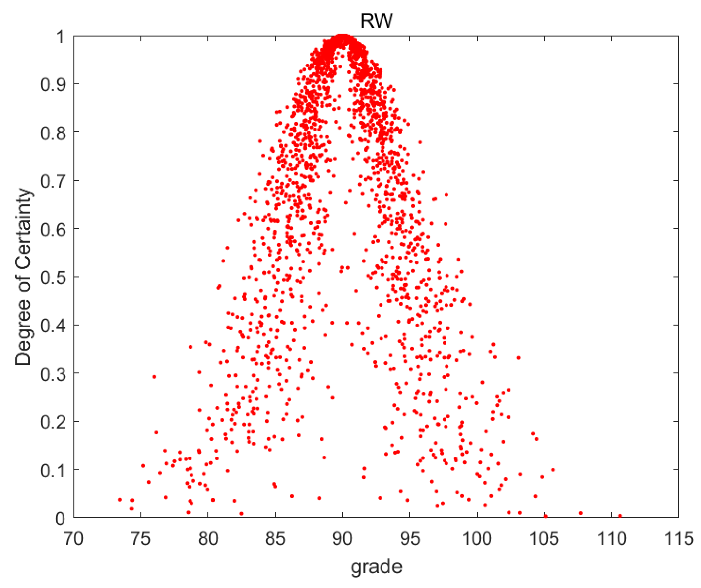
3.1.4. Road Width
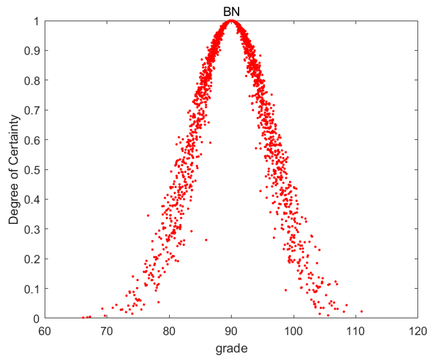
3.1.5. Bridges
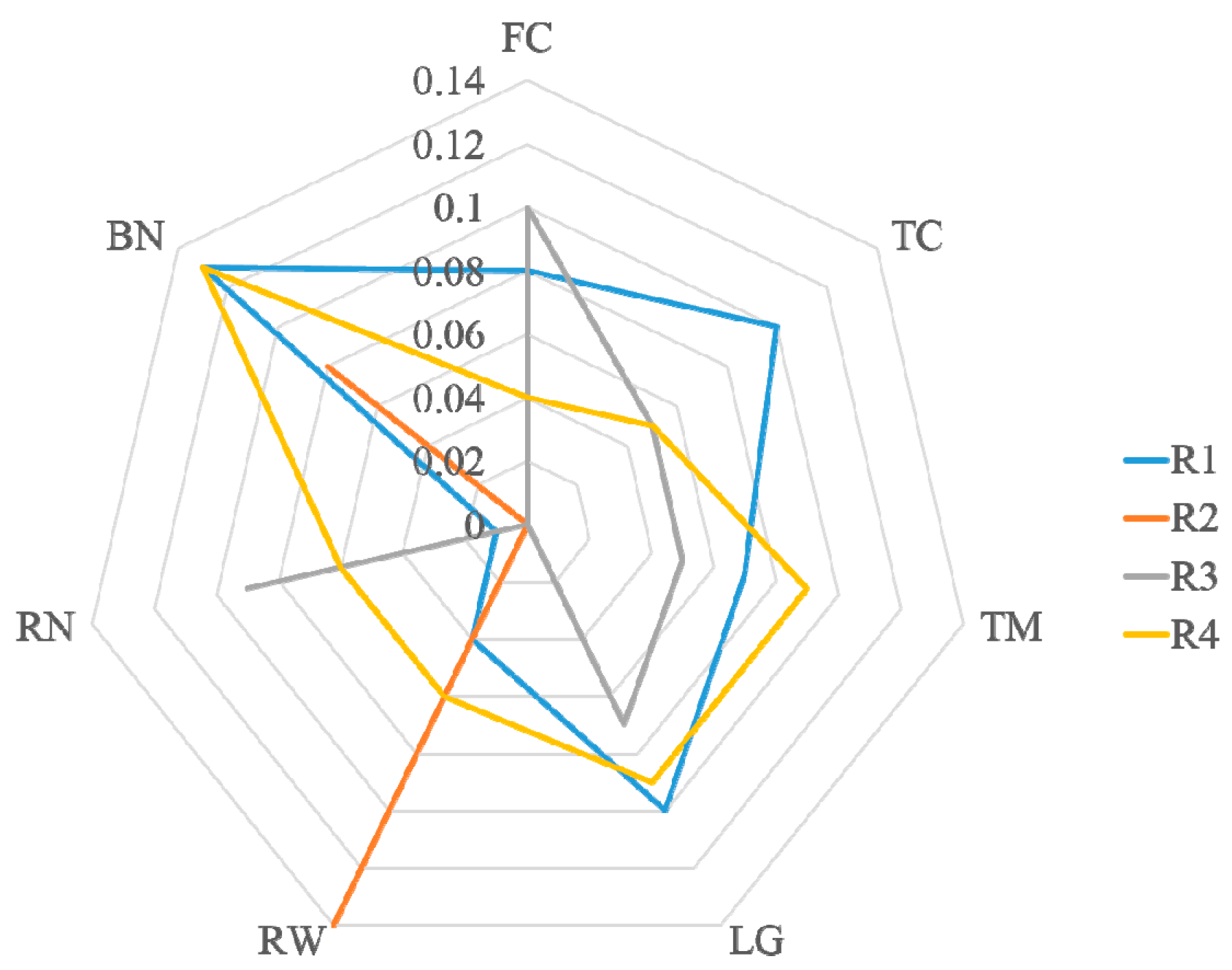
- In all Tables of this paper:
- FC is the number of horizontal curves with a radius less than 20 m.
- TC is the number of switch-back curves.
- TM is the total mileage.
- LG is the road mileage with a longitudinal gradient greater than 5%.
- RW is the road mileage with a width greater than 25 m.
- RN is the road mileage with a width less than 15 m.
- BN is the number of bridges with headroom less than 5 m.
3.2. Weight Calculation
3.2.1. Standardize
3.2.2. Determine the Weight of Influencing Factor
3.3. Cloud Model Optimization
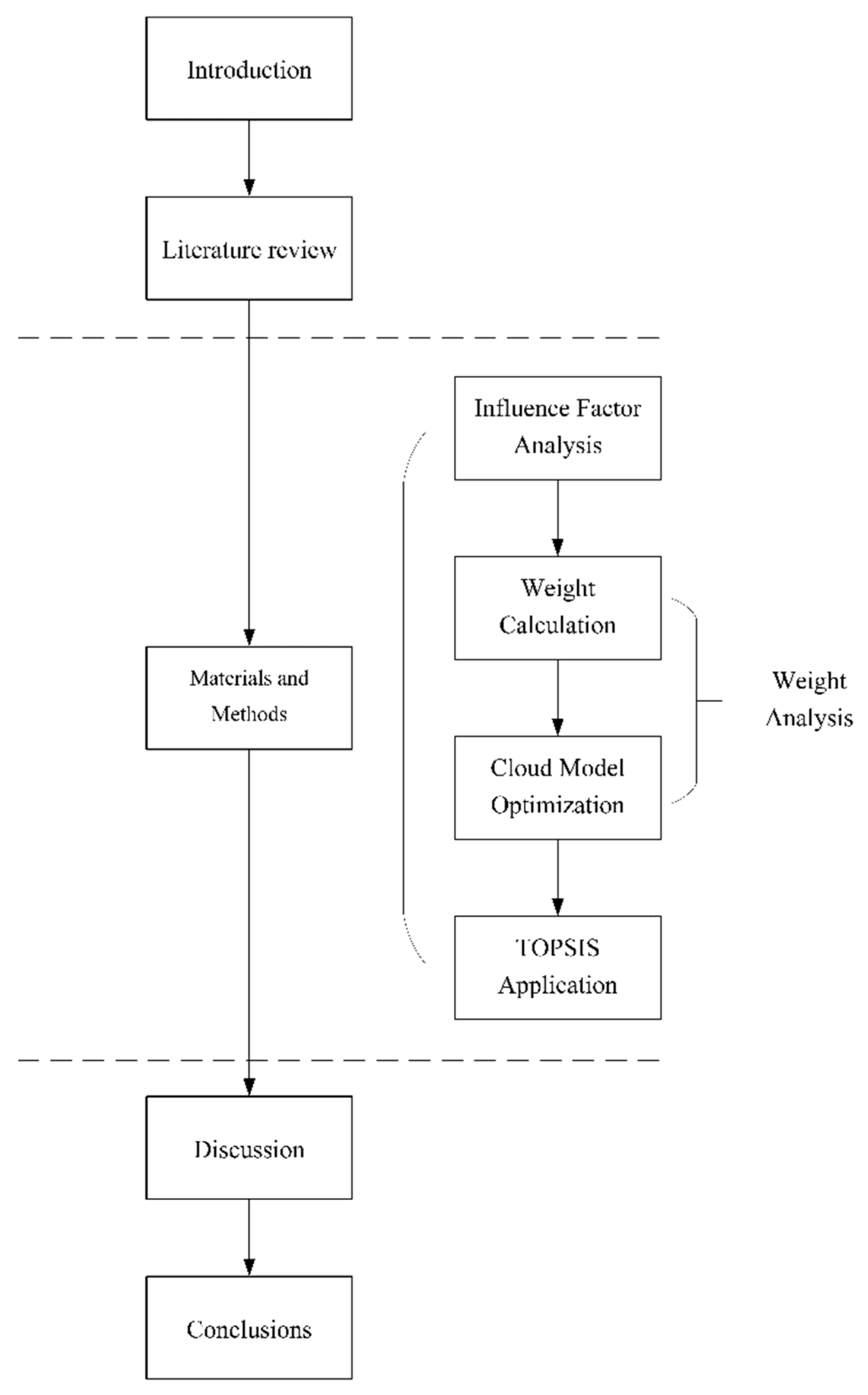
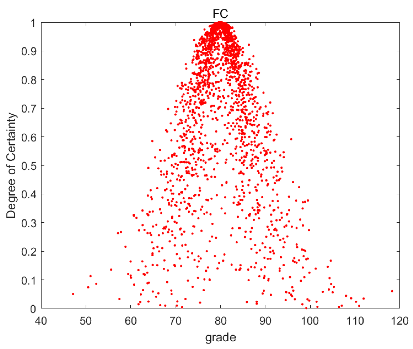
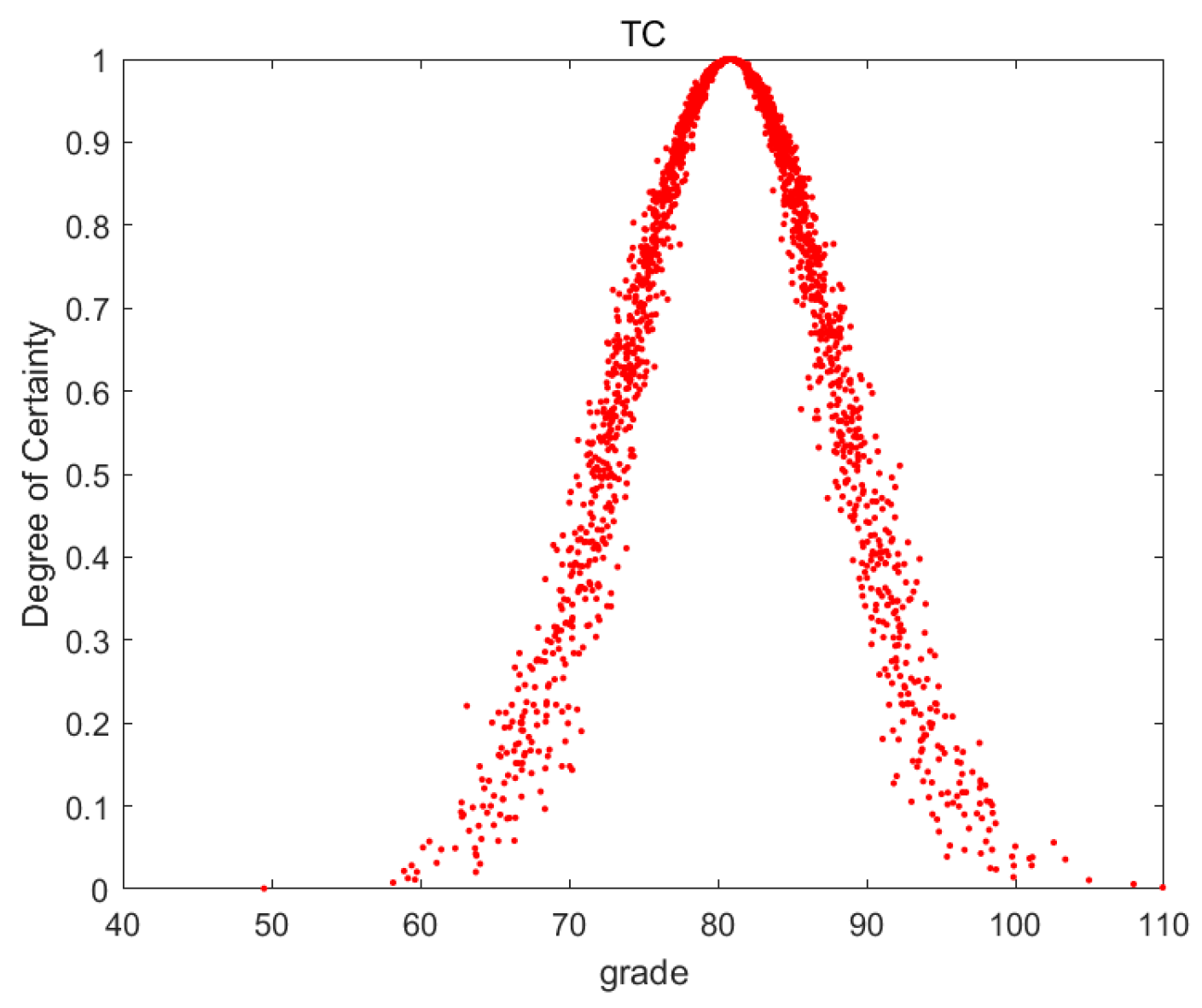
3.3.1. Definition of Cloud Model
3.3.2. Descriptive Statistics of Cloud Model
3.3.3. Backward Cloud Generator
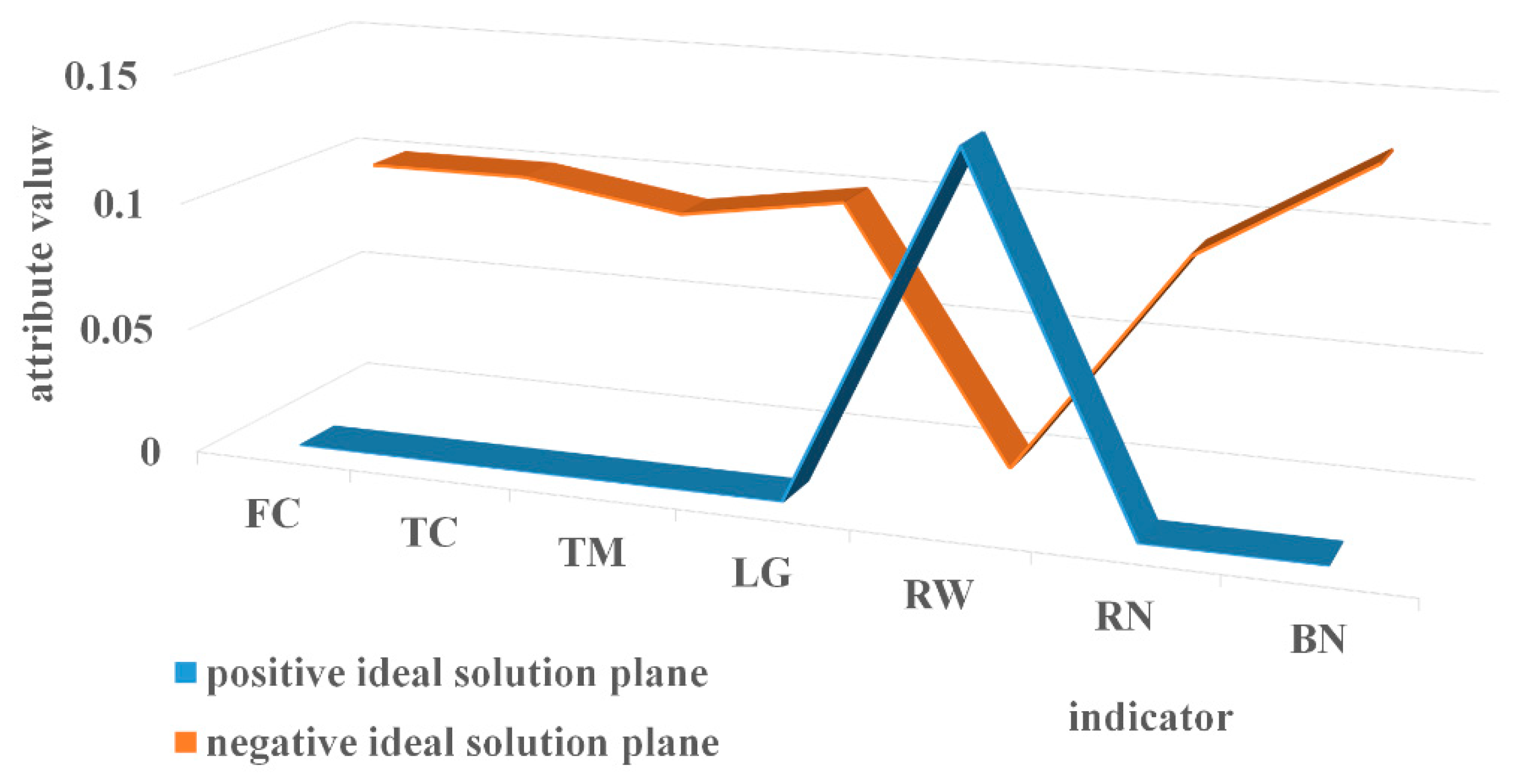
3.4. TOPSIS Application
3.4.1. Step 1
3.4.2. Step 2
3.4.3. Step 3
3.4.4. Step 4
3.4.5. Step 5
4. Discussion
5. Conclusions
- It summarizes the factors that need to be generally considered in urban oversize cargo transportation.
- Based on the characteristics of the cloud model that can reasonably handle subjective evaluation, it can be used to optimize the weight; the objective distribution of the weight is ensured and the subjective opinions of the practitioners are fully considered.
- The weight optimization method combined with TOPSIS is introduced into the field of oversize cargo transportation passing through a city for the first time, providing a new route selection solution. Its Pearson correlation coefficient for actual transportation is 0.018 higher than the entropy weight–TOPSIS method and 0.057 higher than the TOPSIS method.
Author Contributions
Funding
Institutional Review Board Statement
Informed Consent Statement
Data Availability Statement
Conflicts of Interest
References
- Meng, L.; Hu, Z.; Huang, C.; Zhang, W.; Jia, T. Optimized Route Selection Method based on the Turns of Road Intersections: A Case Study on Oversized Cargo Transportation. ISPRS Int. J. Geo-Inf. 2015, 4, 2428–2445. [Google Scholar] [CrossRef]
- Petraška, A.; Čižiūnienė, K.; Jarašūnienė, A.; Maruschak, P.; Prentkovskis, O. Algorithm for the assessment of heavyweight and oversize cargo transportation routes. J. Bus. Econ. Manag. 2017, 18, 1098–1114. [Google Scholar] [CrossRef][Green Version]
- Bazaras, D.; Batarlienė, N.; Palsaitis, R.; Petraška, A. Optimal road route selection criteria system for oversize goods transportation. Balt. J. Road Bridg. Eng. 2013, 8, 19–24. [Google Scholar] [CrossRef]
- Wolnowska, A.E.; Konicki, W. Multi-criterial analysis of oversize cargo transport through the city, using the AHP method. Transp. Res. Procedia 2019, 39, 614–623. [Google Scholar] [CrossRef]
- Luo, Y.; Zhang, Y.; Huang, J.; Yang, H. Multi-route planning of multimodal transportation for oversize and heavyweight cargo based on reconstruction. Comput. Oper. Res. 2021, 128, 105172. [Google Scholar] [CrossRef]
- Koohathongsumrit, N.; Meethom, W. An integrated approach of fuzzy risk assessment model and data envelopment analysis for route selection in multimodal transportation networks. Expert Syst. Appl. 2021, 171, 114342. [Google Scholar] [CrossRef]
- Pamucar, D.; Ćirović, G. Vehicle route selection with an adaptive neuro fuzzy inference system in uncertainty conditions. Decis. Mak. Appl. Manag. Eng. 2018, 1, 13–37. [Google Scholar] [CrossRef]
- Ma, C.; Hao, W.; He, R.; Moghimi, B. A Multiobjective Route Robust Optimization Model and Algorithm for Hazmat Transportation. Discret. Dyn. Nat. Soc. 2018, 2018, 1–12. [Google Scholar] [CrossRef]
- Herrera, I.A.; Rogier, W. Comparing a multi-linear (STEP) and systemic (FRAM) method for accident analysis. Reliab. Eng. Syst. Saf. 2010, 95, 1269–1275. [Google Scholar] [CrossRef]
- Zhu, X.; Zhang, P.; Wei, Y.; Li, Y.; Zhao, H. Measuring the efficiency and driving factors of urban land use based on the DEA method and the PLS-SEM model—A case study of 35 large and medium-sized cities in China. Sustain. Cities Soc. 2019, 50, 101646. [Google Scholar] [CrossRef]
- Campisi, T.; Socrates, B.; Tesoriere, G.; Trouva, M.; Papas, T.; Mrak, I. How to Create Walking Friendly Cities. A Multi-Criteria Analysis of the Central Open Market Area of Rijeka. Sustainability 2020, 12, 9470. [Google Scholar] [CrossRef]
- Huang, W.; Zhang, Y.; Yu, Y.; Xu, Y.; Xu, M.; Zhang, R.; De Dieu, G.J.; Yin, D.; Liu, Z. Historical data-driven risk assessment of railway dangerous goods transportation system: Comparisons between Entropy Weight Method and Scatter Degree Method. Reliab. Eng. Syst. Saf. 2021, 205, 107236. [Google Scholar] [CrossRef]
- Guo, S. Application of Entropy Weight Method in the Evaluation of the Road Capacity of Open Area; MEP: Hangzhou, China, 2017; Volume 1839, p. 20120. [Google Scholar]
- Xu, H.; Ma, C.; Lian, J.; Xu, K.; Chaima, E. Urban flooding risk assessment based on an integrated k-means cluster algorithm and improved entropy weight method in the region of Haikou, China. J. Hydrol. 2018, 563, 975–986. [Google Scholar] [CrossRef]
- Gorgij, A.D.; Kisi, O.; Moghaddam, A.A.; Taghipour, A. Groundwater quality ranking for drinking purposes, using the entropy method and the spatial autocorrelation index. Environ. Earth Sci. 2017, 76, 269. [Google Scholar] [CrossRef]
- Lianxiao; Morimoto, T. Spatial Analysis of Social Vulnerability to Floods Based on the MOVE Framework and Information Entropy Method: Case Study of Katsushika Ward, Tokyo. Sustainability 2019, 11, 529. [Google Scholar] [CrossRef]
- Islam, A.R.M.T.; Ahmed, N.; Doza, B.; Chu, R. Characterizing groundwater quality ranks for drinking purposes in Sylhet district, Bangladesh, using entropy method, spatial autocorrelation index, and geostatistics. Environ. Sci. Pollut. Res. 2017, 24, 26350–26374. [Google Scholar] [CrossRef]
- Sahoo, M.M.; Patra, K.; Swain, J.; Khatua, K.K. Evaluation of water quality with application of Bayes’ rule and entropy weight method. Eur. J. Environ. Civ. Eng. 2016, 21, 730–752. [Google Scholar] [CrossRef]
- Zhao, H.; Yao, L.; Mei, G.; Liu, T.; Ning, Y. A Fuzzy Comprehensive Evaluation Method Based on AHP and Entropy for a Landslide Susceptibility Map. Entropy 2017, 19, 396. [Google Scholar] [CrossRef]
- Fang, R.; Shang, R.; Wang, Y.; Guo, X. Identification of vulnerable lines in power grids with wind power integration based on a weighted entropy analysis method. Int. J. Hydrogen Energy 2017, 42, 20269–20276. [Google Scholar] [CrossRef]
- Romero, I.; Delgado, A. Applying grey systems and shannon entropy to social impact assessment and environmental conflict analysis. Int. J. Appl. Eng. Res. 2017, 12, 14327–14337. [Google Scholar]
- Feng, J.; Gong, Z. Integrated linguistic entropy weight method and multi-objective programming model for supplier selection and order allocation in a circular economy: A case study. J. Clean. Prod. 2020, 277, 122597. [Google Scholar] [CrossRef]
- Ren, Z. Evaluation Method of Port Enterprise Product Quality Based on Entropy Weight TOPSIS. J. Coast. Res. 2020, 103, 766–769. [Google Scholar] [CrossRef]
- Wang, B.; Liu, J. Comprehensive Evaluation and Analysis of Maritime Soft Power Based on the Entropy Weight Method (EWM); CISAT: Daqing, China, 2019; Volume 1168, p. 032108. [Google Scholar]
- Duan, K.; Zuo, J.; Zhao, X.; Tang, D. Integrated Sustainability Assessment of Public Rental Housing Community Based on a Hybrid Method of AHP-Entropy Weight and Cloud Model. Sustainability 2017, 9, 603. [Google Scholar] [CrossRef]
- Gong, Y.; Chen, L. Trust Evaluation of User Behavior Based on Entropy Weight Method; CENet: Xi’an, China, 2020; pp. 670–675. [Google Scholar]
- Delgado, A.; Ayala, B.; Carbajal, C. An Approach to Analyse Social Development in South America by Shannon Entropy Theory; CHILECON: Valparaiso, Chile, 2019; pp. 1–5. [Google Scholar]
- Delgado, A.; Carbajal, C.; Reyes, H.; Romero, I. Social Impact Assessment on a Mining Project in Peru Using the Grey Clustering Method and the Entropy-Weight Method; ColCACI: Barranquilla, Colombia, 2019; pp. 116–128. [Google Scholar]
- Lu, J.; Wang, W.; Zhang, Y.; Cheng, S. Multi-Objective Optimal Design of Stand-Alone Hybrid Energy System Using Entropy Weight Method Based on HOMER. Energies 2017, 10, 1664. [Google Scholar] [CrossRef]
- Zhao, G.; Wang, D. Comprehensive evaluation of AC/DC hybrid microgrid planning based on analytic hierarchy process and entropy weight method. Appl. Sci. 2019, 9, 3843. [Google Scholar] [CrossRef]
- Zhou, S.-J.; Tan, M.; Wang, X.-D.; Yang, Y.-B.; Zhang, X.-X. Comprehensive Effectiveness Evaluation Based on Entropy Weight Method for Energy Utilization Schemes of Smart Parks; EEA: Hong Kong, China, 2017; pp. 326–332. [Google Scholar]
- Liao, X.; Xue, M.; Mao, X.; Pan, Y.; Sun, G.; Wei, Z. Risk Assessment of Integrated Electricity--Heat Energy System with Cross Entropy and Objective Entropy Weight Method; ACPEE: Chengdu, China, 2020; pp. 94–99. [Google Scholar]
- Xu, T.; Qin, C.; Zhang, H.; Qu, Y.; Fang, W. Study on Petroleum Standard Attention Index Calculation based on the Entropy Weight Method. IOP Conf. Ser. Earth Environ. Sci. 2020, 514, 514. [Google Scholar] [CrossRef]
- Muqeem, M.; Sherwani, A.F.; Ahmad, M.; Khan, Z.A. Application of the Taguchi based entropy weighted TOPSIS method for optimisation of diesel engine performance and emission parameters. Int. J. Heavy Veh. Syst. 2019, 26, 69. [Google Scholar] [CrossRef]
- Bai, H.; Feng, F.; Wang, J.; Wu, T. A Combination Prediction Model of Long-Term Ionospheric foF2 Based on Entropy Weight Method. Entropy 2020, 22, 442. [Google Scholar] [CrossRef] [PubMed]
- Zhao, J.; Wu, D.; Zhang, Y.; Wang, M. Extension evaluation of green building Project Management performance based on entropy weight method. J. Eng. Manag. 2018, 32, 125–130. [Google Scholar]
- Du, Y.; Zheng, Y.; Wu, G.; Tang, Y. Decision-making method of heavy-duty machine tool remanufacturing based on AHP-entropy weight and extension theory. J. Clean. Prod. 2020, 252, 119607. [Google Scholar] [CrossRef]
- Song, M.; Zhu, Q.; Peng, J.; Gonzalez, E.D.S. Improving the evaluation of cross efficiencies: A method based on Shannon entropy weight. Comput. Ind. Eng. 2017, 112, 99–106. [Google Scholar] [CrossRef]
- Han, Y.M.; Fang, D.; Zhang, H.Y.; Li, Y. Efficiency Evaluation of Intelligent Swarm Based on AHP Entropy Weight Method; CISAI: Inner Mongolia, China, 2020; p. 012072. [Google Scholar]
- Qi, X.; Zhou, M. Integrated Energy Service Demand Evaluation Based on AHP and Entropy Weight Method; ICEEB: Xi’an, China, 2020; Volume 185, p. 01046. [Google Scholar]
- Wu, Z.; Chen, G.; Yao, J. The Stock Classification Based on Entropy Weight Method and Improved Fuzzy C-Means Algorithm; ICBDC: Guangzhou, China, 2019; pp. 130–134. [Google Scholar]
- Lu, J.; Wei, C.; Wu, J.; Wei, G. TOPSIS Method for Probabilistic Linguistic MAGDM with Entropy Weight and Its Application to Supplier Selection of New Agricultural Machinery Products. Entropy 2019, 21, 953. [Google Scholar] [CrossRef]
- Dos Santos, B.M.; Godoy, L.P.; Campos, L.M. Performance evaluation of green suppliers using entropy-TOPSIS-F. J. Clean. Prod. 2019, 207, 498–509. [Google Scholar] [CrossRef]
- Kumar, R.; Singh, S.; Bilga, P.S.; Jatin, K.; Singh, J.; Singh, S.; Scutaru, M.-L.; Pruncu, C.I. Revealing the benefits of entropy weights method for multi-objective optimization in machining operations: A critical review. J. Mater. Res. Technol. 2021, 10, 1471–1492. [Google Scholar] [CrossRef]
- Zhao, H.; Li, N. Risk Evaluation of a UHV Power Transmission Construction Project Based on a Cloud Model and FCE Method for Sustainability. Sustainability 2015, 7, 2885–2914. [Google Scholar] [CrossRef]
- Liu, H.-C.; Wang, L.-E.; Li, Z.; Hu, Y.-P. Improving Risk Evaluation in FMEA with Cloud Model and Hierarchical TOPSIS Method. IEEE Trans. Fuzzy Syst. 2019, 27, 84–95. [Google Scholar] [CrossRef]
- Wang, S.; Zhang, L.; Ma, N.; Wang, S. An Evaluation Approach of Subjective Trust Based on Cloud Model; CSSE: Wuhan, China, 2008; pp. 1062–1068. [Google Scholar]
- Zhang, T.; Yan, L.; Yang, Y. Trust evaluation method for clustered wireless sensor networks based on cloud model. Wirel. Netw. 2018, 24, 777–797. [Google Scholar] [CrossRef]
- Li, L.; Liu, L.; Yang, C.; Li, Z. The Comprehensive Evaluation of Smart Distribution Grid Based on Cloud Model. Energy Procedia 2012, 17, 96–102. [Google Scholar] [CrossRef]
- Wang, J.-Q.; Peng, J.-J.; Zhang, H.-Y.; Liu, T.; Chen, X.-H. An Uncertain Linguistic Multi-criteria Group Decision-Making Method Based on a Cloud Model. Group Decis. Negot. 2015, 24, 171–192. [Google Scholar] [CrossRef]
- Li, Y.; Liu, X.; Chen, Y. Selection of logistics center location using Axiomatic Fuzzy Set and TOPSIS methodology in logistics management. Expert Syst. Appl. 2011, 38, 7901–7908. [Google Scholar] [CrossRef]
- Abdel-Basset, M.; Mohamed, R. A novel plithogenic TOPSIS-CRITIC model for sustainable supply chain risk management. J. Clean. Prod. 2020, 247, 119586. [Google Scholar] [CrossRef]
- Rostamzadeh, R.; Ghorabaee, M.K.; Govindan, K.; Esmaeili, A.; Nobar, H.B.K. Evaluation of sustainable supply chain risk management using an integrated fuzzy TOPSIS- CRITIC approach. J. Clean. Prod. 2018, 175, 651–669. [Google Scholar] [CrossRef]
- Sirisawat, P.; Kiatcharoenpol, T. Fuzzy AHP-TOPSIS approaches to prioritizing solutions for reverse logistics barriers. Comput. Ind. Eng. 2018, 117, 303–318. [Google Scholar] [CrossRef]
- Gandhi, N.S.; Thanki, S.J.; Thakkar, J.J. Ranking of drivers for integrated lean-green manufacturing for Indian manufacturing SMEs. J. Clean. Prod. 2018, 171, 675–689. [Google Scholar] [CrossRef]
- Abdel-Basset, M.; Manogaran, G.; Gamal, A.; Smarandache, F. A Group Decision Making Framework Based on Neutrosophic TOPSIS Approach for Smart Medical Device Selection. J. Med Syst. 2019, 43, 38. [Google Scholar] [CrossRef] [PubMed]
- Kelemenis, A.; Askounis, D. A new TOPSIS-based multi-criteria approach to personnel selection. Expert Syst. Appl. 2010, 37, 4999–5008. [Google Scholar] [CrossRef]
- Oztaysi, B. A decision model for information technology selection using AHP integrated TOPSIS-Grey: The case of content management systems. Knowl. Based Syst. 2014, 70, 44–54. [Google Scholar] [CrossRef]
- Fu, Z.; Liao, H. Unbalanced double hierarchy linguistic term set: The TOPSIS method for multi-expert qualitative decision making involving green mine selection. Inf. Fusion 2019, 51, 271–286. [Google Scholar] [CrossRef]
- Nyimbili, P.H.; Erden, T.; Karaman, H. Integration of GIS, AHP and TOPSIS for earthquake hazard analysis. Nat. Hazards 2018, 92, 1523–1546. [Google Scholar] [CrossRef]
- Mi, Z.-F.; Wei, Y.-M.; He, C.-Q.; Li, H.-N.; Yuan, X.-C.; Liao, H. Regional efforts to mitigate climate change in China: A multi-criteria assessment approach. Mitig. Adapt. Strateg. Glob. Chang. 2017, 22, 45–66. [Google Scholar] [CrossRef]
- Coban, A.; Ertis, I.F.; Cavdaroglu, N.A. Municipal solid waste management via multi-criteria decision making methods: A case study in Istanbul, Turkey. J. Clean. Prod. 2018, 180, 159–167. [Google Scholar] [CrossRef]
- SafarianZengir, V.; Sobhani, B.; Asghari, S. Modeling and Monitoring of Drought for forecasting it, to Reduce Natural hazards Atmosphere in western and north western part of Iran, Iran. Air Qual. Atmos. Health 2019, 13, 119–130. [Google Scholar] [CrossRef]
- Yoon, K.P.; Kim, W.K. The behavioral TOPSIS. Expert Syst. Appl. 2017, 89, 266–272. [Google Scholar] [CrossRef]
- Akram, M.; Adeel, A. TOPSIS Approach for MAGDM Based on Interval-Valued Hesitant Fuzzy N-Soft Environment. Int. J. Fuzzy Syst. 2018, 21, 993–1009. [Google Scholar] [CrossRef]
- Zhang, M.; Li, G.-X. Combining TOPSIS and GRA for supplier selection problem with interval numbers. J. Central South Univ. 2018, 25, 1116–1128. [Google Scholar] [CrossRef]
- Hanif, M.; Nishikant, M.; Sameer, K. A novel TOPSIS–CBR goal programming approach to sustainable healthcare treatment. Ann. Oper. Res. 2018, 1–23. [Google Scholar] [CrossRef]
- Sangaiah, A.K.; Gopal, J.; Basu, A.; Subramaniam, P.R. An integrated fuzzy DEMATEL, TOPSIS, and ELECTRE approach for evaluating knowledge transfer effectiveness with reference to GSD project outcome. Neural Comput. Appl. 2017, 28, 111–123. [Google Scholar] [CrossRef]


| Route Section | FC (Quantity) | TC (Quantity) | TM (Kilometer) | LG (Kilometer) | RW (Kilometer) | RN (Kilometer) | BN (Quantity) |
|---|---|---|---|---|---|---|---|
| R1 | 4 | 0 | 23.13 | 2.45 | 7.01 | 4.3 | 5 |
| R2 | 8 | 2 | 25.3 | 5.12 | 10.1 | 4.71 | 7 |
| R3 | 3 | 1 | 23.77 | 3.34 | 5.77 | 1.22 | 10 |
| R4 | 6 | 1 | 22.58 | 2.8 | 7.48 | 2.15 | 5 |
| Factor | Minimum | Maximum | Mean | Standard Deviation |
|---|---|---|---|---|
| FC | 3 | 8 | 5.25 | 2.21736 |
| TC | 0 | 2 | 1 | .8165 |
| TM | 22.58 | 25.3 | 23.695 | 1.17532 |
| LG | 2.45 | 5.12 | 3.4275 | 1.18624 |
| RW | 5.77 | 10.1 | 7.59 | 1.82218 |
| RN | 1.22 | 4.71 | 3.095 | 1.68017 |
| BN | 5 | 10 | 6.75 | 2.36291 |
| Factor | Information Entropy | Weight |
|---|---|---|
| FC | 0.676 | 0.129 |
| TC | 0.750 | 0.100 |
| TM | 0.658 | 0.137 |
| LG | 0.587 | 0.165 |
| RW | 0.686 | 0.125 |
| RN | 0.707 | 0.117 |
| BN | 0.432 | 0.227 |
| Practitioners Number | FC | TC | TM | LG | RW | RN | BN |
|---|---|---|---|---|---|---|---|
| 1 | 80 | 85 | 60 | 75 | 85 | 50 | 90 |
| 2 | 90 | 85 | 70 | 80 | 90 | 60 | 85 |
| 3 | 80 | 80 | 65 | 75 | 95 | 65 | 85 |
| 4 | 75 | 70 | 50 | 70 | 85 | 50 | 85 |
| 5 | 85 | 90 | 60 | 70 | 95 | 70 | 95 |
| 6 | 70 | 75 | 50 | 65 | 90 | 65 | 100 |
| Factor | |||
|---|---|---|---|
| FC | 80 | 6.27 | 3.28 |
| TC | 80.83 | 7.31 | 0.85 |
| TM | 59.17 | 7.66 | 2.35 |
| LG | 72.5 | 5.22 | 0.48 |
| RW | 90 | 4.18 | 1.59 |
| RN | 60 | 8.36 | 0.43 |
| BN | 90 | 6.27 | 0.85 |
| Factor | Weight |
|---|---|
| FC | 0.139 |
| TC | 0.122 |
| TM | 0.121 |
| LG | 0.154 |
| RW | 0.157 |
| RN | 0.110 |
| BN | 0.197 |
| Route Section | ||
|---|---|---|
| R1 | 0.24 | 0.09 |
| R2 | 0.08 | 0.26 |
| R3 | 0.22 | 0.15 |
| R4 | 0.22 | 0.1 |
| Route Section | Relative Proximity | TOPSIS | Entropy Weight–TOPSIS | Optimization Weight–TOPSIS |
|---|---|---|---|---|
| R1 | 0.27 | 0.27 | 0.28 | |
| R2 | 0.69 | 0.73 | 0.77 | |
| R3 | 0.5 | 0.46 | 0.4 | |
| R4 | 0.25 | 0.27 | 0.32 |
| Year | R1 | R2 | R3 | R4 |
|---|---|---|---|---|
| 2016 | 0 | 2 | 1 | 2 |
| 2017 | 0 | 1 | 0 | 0 |
| 2018 | 1 | 1 | 2 | 1 |
| 2019 | 2 | 2 | 1 | 1 |
| 2020 | 0 | 3 | 1 | 1 |
| Method | Pearson Correlation Coefficient |
|---|---|
| TOPSIS | 0.938 |
| Entropy weight–TOPSIS | 0.977 |
| Optimization weight–TOPSIS | 0.995 |
Publisher’s Note: MDPI stays neutral with regard to jurisdictional claims in published maps and institutional affiliations. |
© 2021 by the authors. Licensee MDPI, Basel, Switzerland. This article is an open access article distributed under the terms and conditions of the Creative Commons Attribution (CC BY) license (http://creativecommons.org/licenses/by/4.0/).
Share and Cite
Huang, D.; Han, M. An Optimization Route Selection Method of Urban Oversize Cargo Transportation. Appl. Sci. 2021, 11, 2213. https://doi.org/10.3390/app11052213
Huang D, Han M. An Optimization Route Selection Method of Urban Oversize Cargo Transportation. Applied Sciences. 2021; 11(5):2213. https://doi.org/10.3390/app11052213
Chicago/Turabian StyleHuang, Da, and Mei Han. 2021. "An Optimization Route Selection Method of Urban Oversize Cargo Transportation" Applied Sciences 11, no. 5: 2213. https://doi.org/10.3390/app11052213
APA StyleHuang, D., & Han, M. (2021). An Optimization Route Selection Method of Urban Oversize Cargo Transportation. Applied Sciences, 11(5), 2213. https://doi.org/10.3390/app11052213