Severity Classification of Parkinson’s Disease Based on Permutation-Variable Importance and Persistent Entropy

Abstract

Parkinson’s disease (PD) is a neurodegenerative disease that causes chronic and progressive motor dysfunction. As PD progresses, patients show different symptoms at different stages of the disease. The severity assessment is inefficient and subjective when it comes to artificial diagnosis. However, abnormal gait was contingent and the subject selection was limited. Therefore, few-shot learning based on small sample sets is critical to solving the problem of insufficient sample data in PD patients. Using datasets from PhysioNet, this paper presents a method based on permutation-variable importance (PVI) and persistent entropy of topological imprints, and uses support vector machine (SVM) as a classifier to achieve the severity classification of PD patients. The method includes the following steps: (1) Take the data as gait cycles, and calculate the gait characteristics of each cycle. (2) Use the random forest (RF) method to obtain the leading factors differentiating the gait of patients at different severity levels. (3) Use time-delay embedding to map the data into a topological space, and use the topological data analysis based on permutation homology to obtain the persistent entropy. (4) Use the Borderline-SMOTE (BSM) method to balance the sample data. (5) Use the SVM to classify the samples for the severity levels of PD. An accuracy of 98.08% was achieved by 10-fold cross-validation, so our method can be used as an effective means of computer-aided diagnosis of PD, and has important practical value.

1. Introduction

Parkinson’s disease (PD) is a common neurodegenerative disease characterized by the loss of dopamine in neurons in the brain, resulting in a series of complex network dysfunctions [1]. Such dysfunctions may cause significant effects on the gait of patients, such as an unstable walking posture, bradykinesia, tremor dominance, frequent falling, panic gait, and freezing of gait [2]. The onset of PD is a gradual process; in the progression of the disease, clinical patients show different severity. For PD patients with different severities of the disease, there are different means of treatment, so the severity evaluation can greatly strengthen the clinical management of patients by giving the targeted treatment. Currently, the most common PD rating criterion is the Hoehn and Yahr (HY) grading system [3], which divides the severity of PD into five levels (1 to 5, increasing in severity). However, the HY grading evaluation relies heavily on medical experts with specialized knowledge and clinical experiences, which is a time-consuming and low-efficiency process, and inevitably has a certain subjective judgment. Therefore, auxiliary means to assess PD severity is needed to improve the rating efficiency and reduce costs.

With the development of wearable sensing technology, gait-analysis technology based on human sensing data is being increasingly applied in the detection of PD. Among them, the ground reaction force (GRF) is widely used in PD symptom analysis as a common quantitative measurement method for gait assessment [4,5]. As an important indicator of joint movement and muscle activity, the GRF during walking can be obtained by wearable insole sensors, which can well reflect the characteristics of an abnormal gait. These sensors have the advantages of small size, low cost, non-invasiveness, a wide range of application scenarios, and low energy consumption. Muniz et al. [6] used the GRF to evaluate the impacts on PD from the deep brain stimulation of the subthalamic nucleus (DBS-STU) and drug therapy. Petrucci et al. [7] studied the freezing of gait in patients with PD prediction and adjustment, in which the GRF was used as the main evaluation index and the auxiliary effect of ankle orthotics was observed. The ankle orthotics embodied in patients after auxiliary GRF captured significantly lower average vibration amplitude, which indicates that the seriousness of the PD patients is closely related to the GRF. In addition, using musculoskeletal modeling driven by depth sensors, Jeonghoon Oh et al. [8] compared the GRF among patients and healthy people, and found significant differences in the early peaks of the GRF. A large number of studies have shown that the abnormal gait patterns of PD patients are reflected in the GRF during walking, which can be an important feature of the PD research.

The GRF can well reflect the stability of gait, from which we can analyze and grade the severity of PD. Machine learning can effectively solve the problem of medical data analysis, and it has been widely used in related fields. From the perspective of gait data, many related scholars have applied machine-learning methods to conduct classification studies of PD, such as logistic regression, random forest, extreme gradient boosting, radial basis, and neural network [9,10,11,12,13,14,15,16,17,18]. In terms of the PD severity assessment using machine learning, Aite Zhao et al. [19] employed the GRF as gait data to identify the seriousness level using the two-channel method of long short-term memory (LSTM) and convolutional neural network (CNN). Similarly, Wei Zeng et al. [20] used neural networks and other methods for PD severity classification, in which the phase space reconstruction and empirical mode decomposition methods were used in data preprocessing. Balaji E et al. [21] used decision tree (DT), support vector machine (SVM), ensemble classifier (EC), and Bayesian classifier (BC) methods to classify the stages of PD, and achieved an effective evaluation of the severity. In a similar way, Enas Abdulhay et al. [22] and Tun Aurolu et al. [23] achieved effective PD grading by using medium Gaussian SVM and locally weighted random forest methods, respectively, with the shallow-learning method. However, in the above studies, the sample data was small and unbalanced. For instance, in Natasa Kleanthous et al.’s work [9], only 10 PD subjects were involved. In addition, compared with other shallow-learning methods, the deep-learning recognition methods based on neural network showed slightly worse results, with respect to time consumption and effectiveness in distinguishing the similar PD severity levels. The reason for this phenomenon is that deep learning is a supervised learning method based on big data, which relies heavily on a large number of high-quality labeled data. When the data is insufficient, problems such as overfitting occur in the model, thus reducing the recognition rate. Large sample sizes from a limited number of PD patients are associated with high clinical risks, uncontrollable repeatability, and high costs. These reasons make it difficult for many deep-learning models to be applied to PD research. In addition, some gait disorders such as panic gait, short gait, and frozen gait were contingencies in PD patients, which resulted in a small number of negative samples in the body-sensing data. Considering all kinds of factors, the identification of severity level by machine-learning methods is mainly based on small sample datasets, so few-shot learning with a lower sample-data requirement becomes the key to solve the problem.

In addition to few-shot learning, the undersampling and oversampling methods are the common means of balancing a dataset. For a PD disease dataset with too few samples, oversampling is used to expand the dataset, and noise data can be added to enhance the robustness of classifiers. When the model cannot effectively extract features from the existing data, the data can first be processed to find the most important parameters that dominate the differences among classes, or deeper feature analysis of the data can be carried out to make the classification and recognition effect more obvious. Fabienne Reynard et al. [24] studied the dominant factors of stability during treadmill walking, using the random forest (RF) method [25] to measure the importance of the variables, while relatively insignificant variables were removed, which made the analysis more effective. Enas Abdulhay et al. [22] extracted only step time, stance time swing and footstrike profile from the GRF data to analyze and identify the diseases. In addition, in the study of Yan Yan et al. [26], the GRF data were reconstructed in a phase space, after mapping the data to the high-dimensional phase space for topological motion analysis, to study the gait fluctuation, and the extracted topological features were applied. The random forest (RF) method has shown a good performance in permutation-variable importance (PVI) and is widely used [27]. Therefore, RF ranking of the importance of gait characteristics can be used to obtain the main factors influencing the different severity levels in PD patients.

The walking process has strong nonlinear characteristics and can be regarded as a nonlinear dynamic system. Extracting deeper features of gait can enhance the differentiation of samples, which is beneficial to the classification of machine learning. The common method is to use topological data analysis (TDA) to obtain the topological imprint for further feature extraction [20,26].

In the classification of machine learning, traditional classifiers are commonly designed based on balanced datasets, and the losses of classifiers are biased toward the majority of classes [28]. Therefore, the imbalance of sample data may cause the insensitivity of the learning model to a minority of classes. However, in the study of abnormal gait patterns, usually only a small number of samples are available. In the method of balancing samples, the sampling method is often used to balance data, including oversampling [29], undersampling [30], and mixed sampling. In machine learning with a small sample size, the method of oversampling is usually adopted to balance the datasets. Among the oversampling methods, the synthetic minority oversampling technique (SMOTE) is considered to be the most effective [31]. The SMOTE method balances the number of minority classes by interpolation between the adjacent minority class samples, which increases the number of minority class samples and improves the classifier performance [32]. The Borderline-SMOTE method is used to synthesize new samples with only a few samples on the boundary, which can improve the distribution of the samples. However, during the composition of the minority classes, the SMOTE did not consider the class information of the nearest neighbor sample, which often overlays the sample, resulting in poor classification performance. The Borderline-SMOTE method was proposed to improve this problem [33]. Support vector machine (SVM) was first proposed by Vapnik et al. [34] as a solution to the dichotomy problem of linearly separable samples. In terms of recognizing abnormal gait, the SVM was successfully used in various pattern recognition problems [35]. Compared with other traditional learning models, the SVM has an excellent performance in solving few-shot learning problems [36]. Because it adopts the principle of structural risk minimization [37], the SVM model has strong generalization ability.

This paper addresses the PD severity-level classification with a small sample set. The PD gait dataset from Goldberger on PhysioNet [38] was used to demonstrate the proposed method. The dataset consisted of only 29 PD patients (15, 8, and 6 patients with HY ratings of 2, 2.5, and 3, respectively) and 18 healthy controls. The sample data was very small, so we considered three aspects to solve the small-sample learning problem: data, model, and algorithm [39]. When the training samples are insufficient, the neural network model with the objective of minimizing loss function tends to fit on a small number of samples, which results in low generalization capacity. However, many nonparametric methods do not need to train the optimization parameters, such as the embedded-learning (EL) method [40,41]. EL is a nonparametric method based on a measurement in which the prior knowledge of training set is used as a design source. In EL, the samples are embedded into a low-dimensional space, which makes the samples of different categories in the low-dimensional space easier to distinguish. The embedded data then can be enhanced in the aspects of the discrimination degree and the balance among the sample size of classes to optimize the performance of the learner. The GRF data is divided according to the gait cycle, and then the categorized data is processed, and a series of gait characteristics is calculated. The variable importance is evaluated for the obtained characteristics by the RF method, and the variable of a bigger impact on the severity classification is reserved for further distinguishing features.

In order to reconstruct the phase space by embedding the obtained gait characteristics with time delay, the data is mapped to the topological space. The topological characteristics of the obtained point-cloud data are analyzed by using the persistent homology methods to obtain the topological signature of the gait data, such as persistent bar code, persistent scatter plot and persistent state plot. However, these topology imprints are challenging to be used as input to machine learning. For this reason, the persistent scattergram topology marks obtained by important gait parameters is calculated as the persistent entropy [42], which is more suitable for machine learning. The SVM is employed for few-shot learning in gait analysis.

In this study, a method based on permutation-variable importance and persistent entropy is proposed for the severity classification of PD. Based on the small dataset of gait, the dominant factors are extracted by permutation-variable importance, and the persistent entropy is proposed to transform the topological imprints into sample inputs more suitable for machine learning. The proposed method can fully improve the degree of differentiation between different disease categories and achieve a favorable effect, and has certain practical significance.

2. Materials and Methods

2.1. Subjects and Data Set

For this study, we use a gait database from PhysioNet provided by Goldberger [38]. The dataset consisted of GRF signals from PD patients and healthy controls. The gait data signals were collected from normal walking and dual-task walking. The normal walking data of patients and the control group was used in this paper for analysis. There were a total of 47 subjects in this dataset, including 29 PD patients and 18 normal controls. Among the 29 PD patients, there were 20 males and 9 females. The normal control group consisted of 10 males and 8 females. The mean ages of the patients and the control groups were 71 and 72, respectively. Among the PD patients, 15 subjects were HY grade 2, 8 were grade 2.5, and 6 were grade 3.

Table 1. Subject information.

Group	Number	Male	Female	Age	HY = 2	HY = 2.5	HY = 3
PD	29	20	9	71 ± 8	15	8	6
Co	18	10	8	72 ± 6	-	-	-

shows the basic information of the subjects involved in the experiment.

2.2. Analysis Method

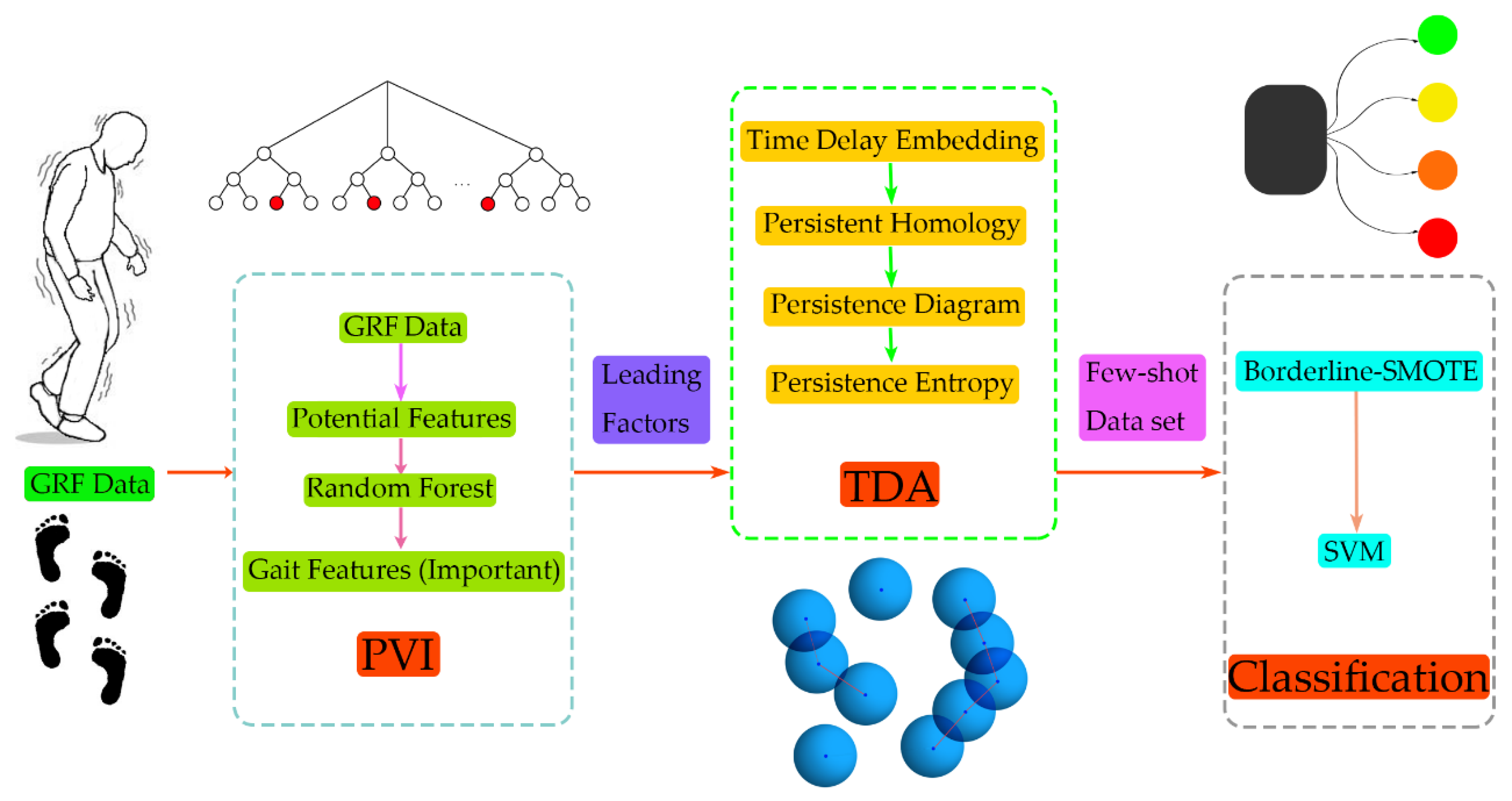
The framework of the proposed method is shown in Figure 1. A total of 47 GRF data (29 PD patients with different disease grades and 18 normal subjects) were used. First, the GRF data were preprocessed, including categorizing subjects according to the gait cycle and calculating the gait characteristics of each gait cycle during walking, then a time series of the gait characteristics was obtained. During the gait-cycle division, the period should be as short as possible on the premise of guaranteeing the complete representation of the gait-cycle information for both the left and right feet. Therefore, we choose two gait cycles as the period and divided them into sections, so that the information in the original signal was completely retained.

Regarding the extraction of gait characteristics on the GRF, we referred to the method on the previous study [43]. In this way, potential characteristics were selected that affected the severity classification, including the coordinates of the center of pressure (CoP), stride time, gait phase, and sample entropy. The random forest method was used to evaluate the importance of these characteristics/variables, and the most significant ones were selected for further analysis. After obtaining the time-series data with a great influence on the difference, the time-delay embedding theorem was used to reconstruct the phase space, and the data were mapped to the phase space to obtain the data point cloud. The topology features of the obtained phase-space-data point cloud were extracted and the persistent entropy was calculated. The Borderline-SMOTE algorithm was used to enhance the data in the training dataset, and the balanced sample data was used as the input to train using SVM to realize the grade recognition of PD.

2.3. Data Description

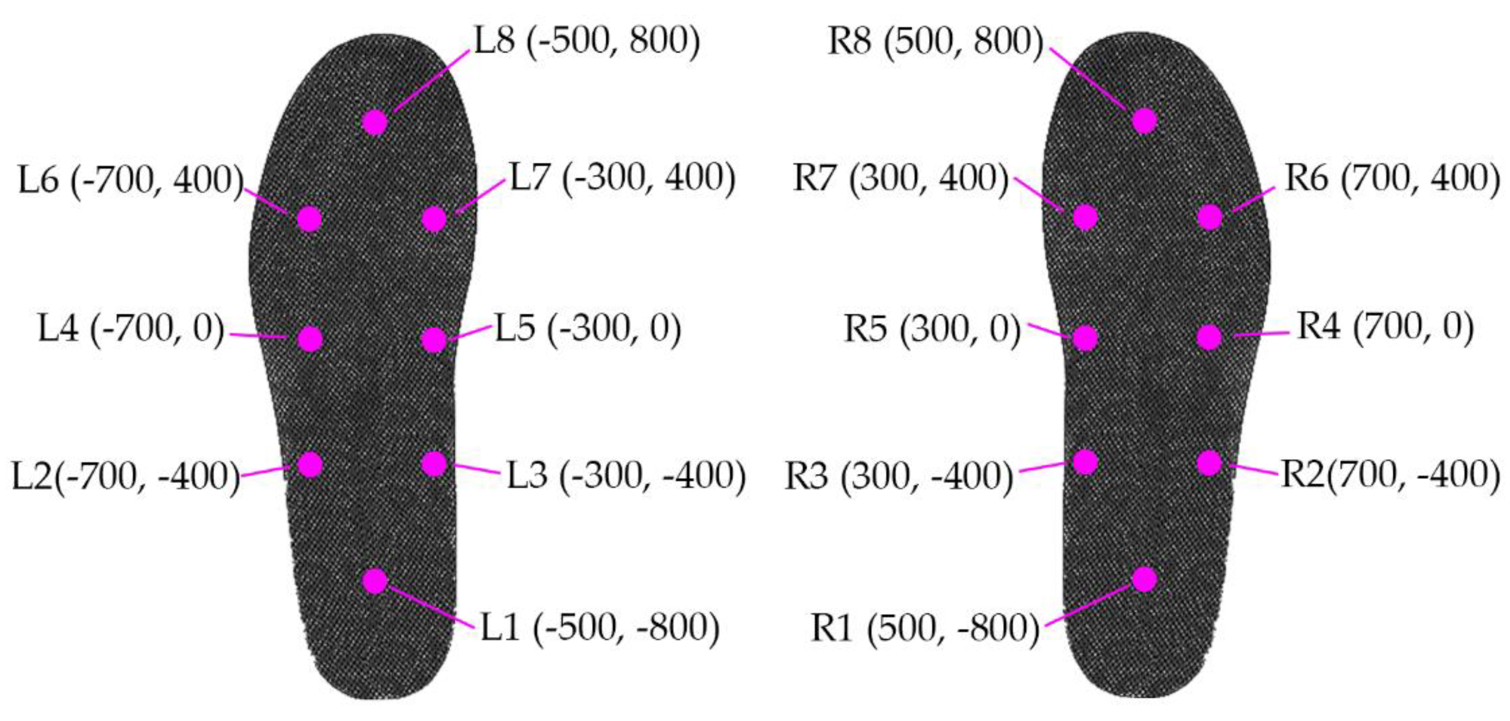
The data recorded were the GRFs when subjects walked for about two minutes on flat ground at a pace of their preference. In the experiments, each subject had 16 force sensors under their feet, with eight sensors under each foot. Thus, we could study stride-to-stride dynamics and the variability of these time series. When a person is comfortable standing with both legs parallel to each other, sensor locations inside the insole can be described approximately in Figure 2, assuming the origin (0,0) is just between the feet, and the person is facing toward the positive Y-axis.

The sampling frequency of the force sensors was 100 Hz, and the forces (N) were collected to obtain a time series of pressure data. In addition to the pressure data, two synthetic signals were generated, including the total sum of the pressure under the left and right feet. The resulting data contain 19 columns per row, with column 1 as time (s); columns 2–9 and 10–17 as the GRF (N) of the left and right feet, respectively; and column 18 as the sum of the GRF on the left foot and column 19 as that for the right. These data were used to fit the relationship between the pressure position and time, model the reaction pressure center as a function of time, and obtain the gait features such as stride time, swing time, etc.

2.4. Preprocessing

2.4.1. Data Partitioning

In this study, the dataset contained 16 independent force sensor signals and 2 synthetic pressure signals. The pressure magnitude and the position of a single sensor could not directly reflect the pressure-tracking distribution during the walk alone. To extract the pressure-tracking distribution, the pressure magnitude and position of individual sensors, the total pressure of all sensors are needed. The changing track of the plantar pressure center was calculated as follows.

$$x=\frac{\sum _{i=1}^8{x}_i{F}_i}{F}$$

(1)

$$y=\frac{\sum _{i=1}^8{y}_i{F}_i}{F}$$

(2)

where $x_i$ and $y_i$ are the X-axis and Y-axis coordinates of the $i$-th sensor of a foot, $F_i$ is the force measured by the corresponding sensor, and $F$ is the sum of the pressures under the foot.

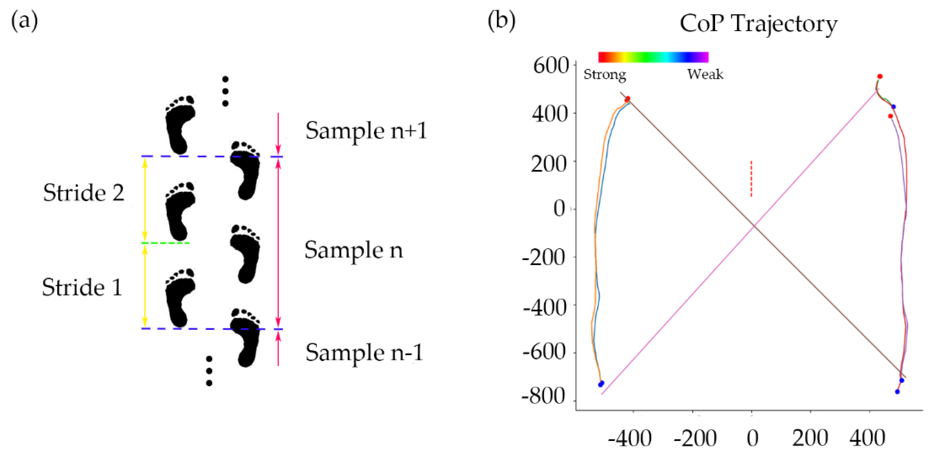
According to the centers of pressure (CoP) obtained in Equations (1) and (2), the entire walking process was divided into two stride cycles. Each cycle began with the first touch of the left heel and ended with the third touch of the same heel (starting the next cycle). This ensured that there was at least one continuous step cycle for each foot. The gait characteristics of each cycle were extracted. The CoP track for each partition is shown in Figure 3. In order to exclude the influence of the unstable features when walking started, the first two stride cycles of each subject were excluded, but the middle 40 dividing cycles and a total of 80 stepping cycles were selected for analysis. The same criteria were applied to each subject to ensure the accuracy of the sampling.

2.4.2. Gait Features

From the track of CoP, we could further extract gait features for better reflection of the characteristics relevant to walking stability in the PD patients. The selected features were screened for visible differences among classes, which was conducive to the inaccurate identification of a small number of classes in the learning of the small sample dataset, so that it could have a better effect on the classifier training of disease grading. The trajectory of CoP was analyzed using linear and nonlinear analysis methods, and the corresponding gait characteristics are obtained; this could further find the most significant factors and realize more accurate grade identification.

In the calculation of the linear characteristics, we used the root mean square (RMS) of the two stride cycles as the results. The linear indicators we selected are as follows:

• CoP distribution and its derivatives. The CoP distribution can well reflect the stability of gait and can be used in the analysis of PD. In the analysis of the coordinate distribution of CoP, we selected the RMS of mediolateral direction (X-axis); anterior–posterior (Y-axis) direction; total CoP coordinates; and the RMS of velocity, acceleration and jerk.
• Gait phase ratio and stride time. In the study of abnormal gait, the proportions of gait time and stride time are usually very important gait characteristics that can clearly reflect the difference between patients and normal subjects. The proportion of the subject’s walking gait can be calculated from the pressure and corresponding time. The length of time between the start of a heel touch on one side and the end of the next heel touch on that side is a step time. Among these, the period from the time when one foot heel touches the ground to the time when the toe is off the ground is the supporting phase of this gait cycle, and the difference between the stride time and the duration of the supporting phase is the swinging phase time of this stride cycle. The proportion of the gait time can be obtained by calculating the time duration of the gait and the time of the stride. The gait phase proportion and stride time of the two stride periods of each division period can be obtained by taking the RMS.
• CoP efficiency and CoP track intersections (CSIP). These two characteristics are also considered, and they may reflect the stability of gait to some extent, and also help us analyze the walking pattern of PD patients. Both of these features can be obtained from the track of CoP. The CoP path efficiency is calculated through dividing direct CoP distance by the actual path that CoP traveled during the stance phase. In the stance phase, the CoP position moves forward under the support foot. When support moves to the other foot, the CoP position moves from one foot to the other [44].

Human walking, as a complex system, has strong nonlinear characteristics. The use of nonlinear analysis method to extract features can effectively analyze the gait characteristics of PD patients. In this study, we chose the sample entropy of CoP as a nonlinear index, which can reflect the degree of disorganization of and attention to walking, and can be used as an important sample input for disease classification and identification.

2.5. Permutation-Variable Importance

When using the small sample dataset to classify the severity of the disease, we chose to first calculate some gait characteristics, in order to find out the characteristics that dominated the difference of different categories and improve the discrimination degree of the samples. For the measurement of the importance of variables, this study used the random forest method to evaluate the importance of features. Using this method, the aim was to identify the dominant factors that influence the different manifestations of PD at different severity levels, and to exclude irrelevant characteristics. The measurement of the importance of variables can reduce the dimension of the input sample data. On one hand, it eliminates the influence of irrelevant factors, while on the other hand, it facilitates the subsequent processing of the data. The random forest method can be used to select the characteristics that have the greatest impact on the severity level, so as to reduce the number of features in the model building and make the classifier achieve good results in training. When we use the random forest method to obtain the importance of certain characteristics in disease classification, the specific steps are as follows:

• For each decision tree, select the corresponding out-of-bag (OOB) data to calculate the out-of-bag data error, which is denoted as $err1$.
• Random noise interference is added to such characteristics of all samples of out-of-bag data, and the out-of-bag data error is calculated again, denoted as $err2$.
• The permutation-variable importance is obtained by Equation (3):

  $$PVI=\frac{\sum _{i=1}^{N}err{2}_i-err{1}_i}{N}$$

  (3)

  where $N$ is the number of decision trees in the random forests, $err{1}_i$ is the OOB error of the $i$-th decision tree for the feature to be evaluated, and $err{2}_i$ is the OOB error of the $i$-th decision tree for an assessment feature after noise interference is added to the feature.

When the random noise is added, the accuracy of data outside the bag will decrease. When this feature is of high importance, the value of OOB error $err{2}_i$ will increase significantly, and the calculated measurement value will increase, indicating that this feature has a great impact on the prediction results of disease grade identification, and thus indicates that this feature is of high importance. In this study, we measured the importance of variables in patients with PD and normal subjects. The results of our assessment of the importance of all the features are shown in Figure 4. We also ranked the evaluation results in order of importance in the two cases, calculated the average value of importance in the two cases, and selected the characteristics that rank in the top 15 for importance.

2.6. Phase-Space Reconstruction

When the time-series data composed of gait features were obtained, we hoped to further extract the difference of features, so as to make the learning effect of classifier more obvious. For patients with PD with a similar grade, the difference in numerical expression of gait characteristics may not be high, and the sample was small, which was likely to affect the recognition accuracy of the classifier. Human walking can be regarded as a complex nonlinear dynamic system. By reconstructing the time series of gait characteristics into a high-dimensional phase space, more abundant information can be mined to achieve the purpose of improving feature discrimination and classification accuracy. The one-dimensional time series corresponding to each gait feature was reconstructed in a phase space, and the data was mapped into a data point cloud in the abstract topological space by the time-delay-embedding method, which can be thought of as sliding a “window” of fixed size over a signal, with each window represented as a point in a (possibly) higher-dimensional space. More formally, given a time series of gait feature $f$, one can extract a sequence of vectors of the form:

$$f_i=[f(t_i),f(t_i+\tau ),\dots ,f(t_i+(d-1)\tau ]$$

(4)

$$s=t_{i+1}-t_i$$

(5)

where $d$ is the embedding dimension and $t$ is the time delay. The quantity $(d-1)t$ is known as the “window size,” and $s$, known as stride, is the difference in $t_{i+1}$ and $t_i$. Then, $T{D}_{d,\tau ,s}$ is the cloud of points where f maps to the phase space with parameters $d$, $\tau$, and $s$:

$$T{D}_{d,\tau ,s}(f)=[f_1,f_2,\dots ,f_n]$$

(6)

In this study, $T{D}_{d,\tau ,s}$ is a numerical time series of multiple gait features. Therefore, too long of a delay will reduce the relevance among elements. Considering the calculation cost and better separability, we chose $d$ = 3, $\tau$ = 1, and $s$ = 1 in this study.

2.7. Topological Data Analysis

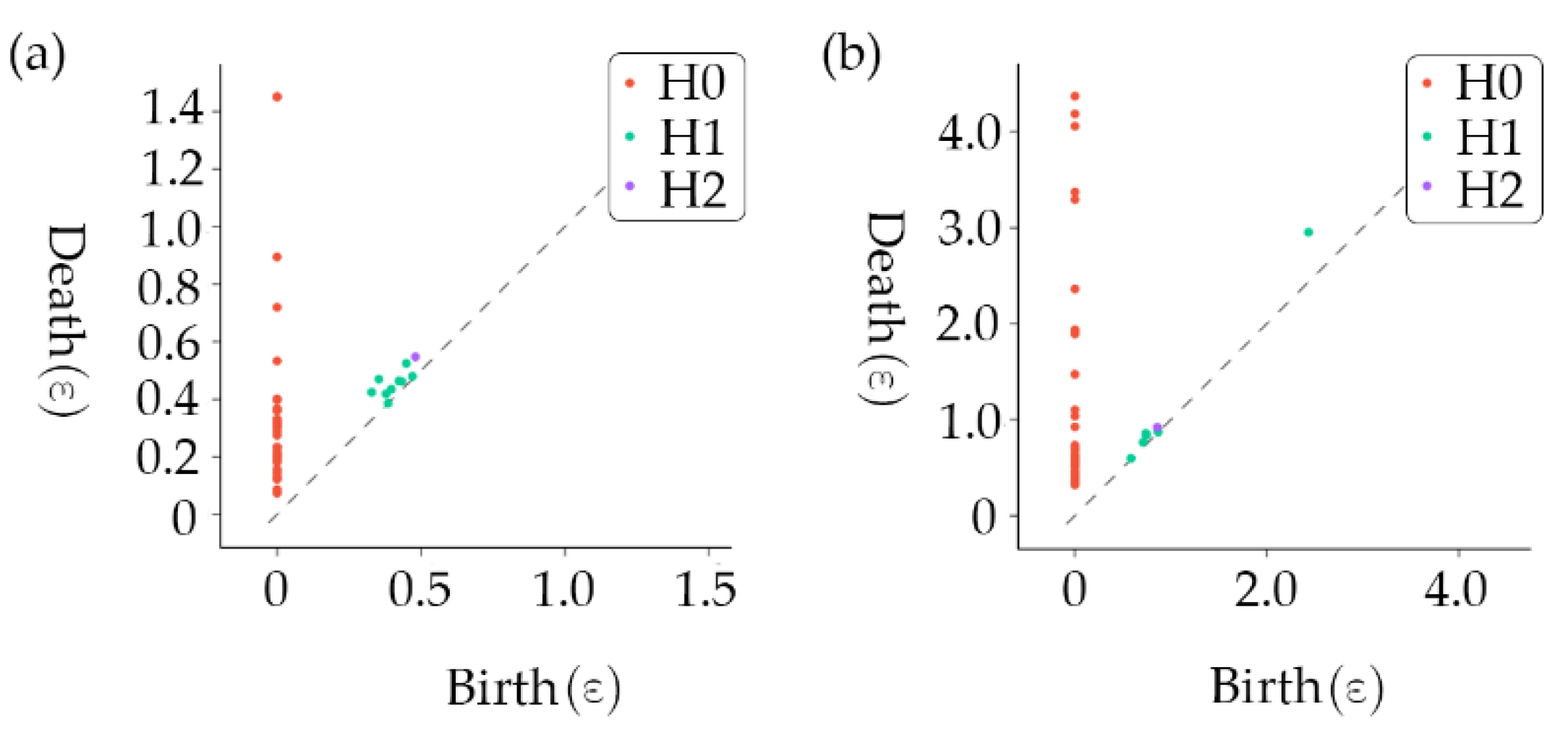
After mapping the time series of the gait characteristics to the topological space, we could extract the relevant topological imprints and apply them to the data analysis. This research adopted a method of topology-imprint analysis based on persistent homology to extract topology features. Each gait characteristic data point mapped to the topological space can be regarded as a small ball with initial radius $\epsilon$ = 0 (0-dimensional homology structure). As $\epsilon$ increases, the balls may intersect and fuse into connectomes (1-dimensional homology), and as $\epsilon$ increases further, the balls may surround holes (2-dimensional homology). However, as the radius of a small sphere $\epsilon$ continues to increase, these connectomes or holes will disappear, which means that these homology structures have a specific duration. We recorded homophones for time of birth and time of death, which we called the persistent homophones, resulting in the topological stamp. A persistence diagram was obtained for each homology structure by plotting a graph with the times of birth and death as the axes, as shown in Figure 5.

However, there was no machine-learning benefit available from persistent scatter diagrams, so we introduced persistent entropy as a treatment:

$$E(D)=-{\displaystyle \sum _{i\in I}{p}_i\log (p_i)}$$

(7)

$$p_i=\frac{d_i-b_i}{L_D}$$

(8)

$$L_D={\displaystyle \sum _{i\in I}(d_i-b_i)}$$

(9)

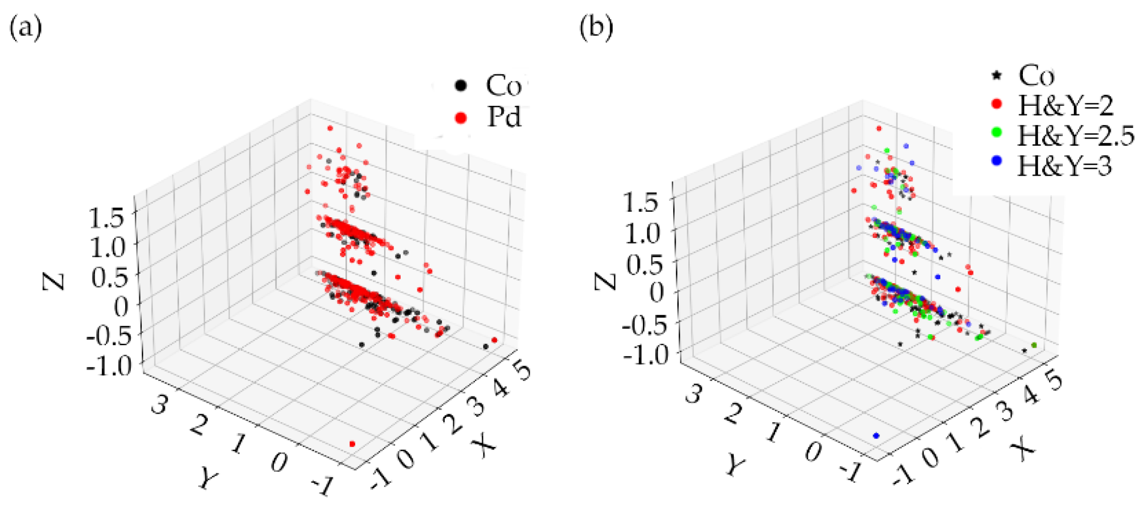
where $I$ is the set of points in a persistence diagram; $b_i$ and $d_i$ are the times of birth and death of the $i$-th point, respectively; and $E(D)$ is the persistent entropy of the persistence diagram $D$. The persistent entropy distribution of control subjects and PD subjects is shown in the Figure 6.

In this way, we represented each persistence diagram as a persistent entropy with three numbers. Thus, the gait characteristics of each subject could be transformed into persistent entropy, which represents the information of each characteristic and greatly reduced the data dimension of the input sample.

2.8. Data Oversampling

According to the above methods, we obtained the persistent entropy of each subject’s gait characteristics as the sample data for the classification training of PD. Obviously, there was still a significant imbalance in the sample data. In the data we used, there were twice and three times as many as grade 2 subjects as there were grade 2.5 and 3 subjects, respectively. Subjects with a severity level of 3 were regarded as the lowest group, accounting for only 20.7% of the total sample dataset. If the data is directly put into the classifier for learning, then the test results of the classifier will be biased to most classes, resulting in the problem of insensitivity to the identification of a few classes, which is very unfavorable to the training of the classifier. In order to avoid this situation, we use Borderline-SMOTE to balance the dataset. The Borderline-SMOTE [33] is an improved oversampling algorithm based on SMOTE that uses only a few class samples on the boundary to achieve the oversampling, thus improving the class distribution of the sample. The specific steps of Borderline-SMOTE are as follows:

• Calculate the Euclidean distance between each sample point $p_i$ and all the training samples, and get the $m$ nearest neighbor of the sample point.
• A small number of samples were divided. Assuming that $m^{\prime }$ of the m nearest neighbor samples belong to most of the samples ($0\le m^{\prime }\le m$), there can be three situations, as follows: when $m^{\prime }=m$, $p_i$ is considered as noise and data synthesis is not performed; when $0\le m^{\prime }\le \frac{m}{2}$, $p_i$ is considered as a safe sample and no data synthesis is performed; when $\frac{m}{2}\le m^{\prime }\le m$, $p_i$ is divided into boundary samples and the data needs to be synthesized, the boundary sample is denoted as:

  $$\{p_1^{\prime },p_{2,\dots }^{\prime }{p}_{dnum}^{\prime }\},(0\le dnum\le pnum)$$

  (10)

  where $dunm$ is the number of minority-class boundary samples and $punm$ is the total number of minority samples.
• The $K$ nearest neighbor between the boundary sample point $p_i$ and the minority sample $P$ is calculated. According to the sampling ratio $U$, $s$ (The number of $s$ is $K$ nearest neighbors multiplied by sampling ratio $U$) and $p{\prime }_i$ are selected for linear interpolation to synthesize a small number of samples.

  $$Synthetic=p_i^{\prime }+r_i\times d_j,(j=1,2,\dots ,s)$$

  (11)

  where $d_j$ identifies the distance between $p_i^{\prime }$ and its $s$ neighbors, and $r_j$ is a random number between 0 and 1.
• A few kinds of synthetic samples and the original training samples are combined to form a new training sample.

By using the Borderline-SMOTE method, the sample set reached a balance of the class, and use the balanced dataset for classifier training in the following step. In this study, we only used the Borderline-SMOTE method during training to enhance the data, but the training set remained unchanged.

2.9. Machine-Learning Method

The classification of PD is essentially a multiclassification problem based on small sample data. To solve the few-shot learning problem, SVM is a novel few-shot learning method with a solid theoretical foundation that can achieve better results than other classifiers on the small sample training set. The reason why SVM has an excellent performance in few-shot learning is that it basically does not involve probability measurements or the law of large numbers. In essence, SVM avoids the traditional process from induction to deduction and achieves efficient classification and regression. At the same time, SVM can also solve the few-shot learning generalization ability, but is not strong. Since the optimization goal of SVM itself is to minimize the structured risk [37] rather than the empirical risk, the concept of the interval is used to obtain the structured description of data distribution, which reduces the requirements for data size and data distribution. This gives SVM an excellent generalization ability. In addition, a small amount of support vectors determines the final result of SVM. Adding or deleting nonsupport vector samples has no effect on the model, which gives the SVM training model good robustness. For PD classification in this study, the dimension of the training sample was higher, and in aiming at this problem, the SVM provided a way to avoid the complexity of the high-dimensional space, the inner product function directly in this space, the kernel function, the solution of the recycling in the case of the linear separable method to directly solve the decision problem of the corresponding higher-dimensional space, and to simplify the solution of the higher-dimensional space problem. Compared with other algorithms such as the neural network, SVM, which is based on the principle of structural risk minimization, avoids overlearning problems, and has a strong generalization ability. SVM is a convex optimization problem, so the local optimal solution must be the global optimal solution.

SVM is a learning device to dichotomize linearly separable samples. In this study, we used the radial basis function (RBF) to convert the samples to the state of linear-separable or approximate linear-separable. The classification of PD is a multiclassification problem. The strategy of one vs. one (OvO) or one vs. rest (OvR) and a dichotomous classification algorithm can be adapted to classify PD using SVM. In this study, we need to classify 4 types of samples from 3 different classes of patients and normal subjects. OvR’s method is to take one sample as a class and treat the remaining samples of all types as another class to form four dichotomous problems and train a total of four models. OvO’s method combines two classes of samples each time to form six dichotomous problems and train a total of six models. When we classify, the samples to be tested are passed into all models, and the corresponding result of the model with the highest probability is the final result. Obviously, the OvO method has a higher accuracy, but it also takes a longer time. In this study, the sample size was small and there was no significant difference in the number of models generated by the two strategies, so we chose the OvO strategy with higher accuracy to solve the multiclassification problem of SVM.

2.10. Statistics

In this study, the classification of PD was a multiclassification problem. When evaluating the performance of the classifier, we paid more attention to the recognition accuracy and misjudgment between categories, in addition to the recognition accuracy of each category. In the evaluation of multiple categories, we transformed the problem of multiple categories into the problem of multiple dichotomies for performance evaluation. In this study, five indicators were used to evaluate the performance of the classifier, including global accuracy, single-class precision, single-class recall, inter-class precision, and inter-class recall. In the following equations, $T$ indicates the classification is correct and $F$ indicates the classification is incorrect, and $P$ and $N$ indicate whether the sample is positive or negative, respectively.

$$accuracy=\frac{ncorrect}{N}$$

(12)

where $accuracy$ is global accuracy, $ncorrect$ is the number of all predicted correct samples, and $N$ is the total number of samples.

$$P_{class}=\frac{T{P}_{class}}{T{P}_{class}+F{P}_{class}}$$

(13)

$$R_{class}=\frac{T{P}_{class}}{T{P}_{class}+F{N}_{class}}$$

(14)

where $P_{class}$ and $R_{class}$ are single-class precision and single-class recall, and class is the category to be evaluated.

$$P_{p-n}=\frac{T{P}_{p-n}}{T{P}_{p-n}+F{P}_{p-n}}$$

(15)

$$R_{p-n}=\frac{T{P}_{p-n}}{T{P}_{p-n}+F{N}_{p-n}}$$

(16)

where $P_{p-n}$ and $R_{p-n}$ are inter-class precision and inter-class recall, $p$ represents the positive class, and $n$ represents the negative class.

3. Results

3.1. SVM Classification

The data processing and classification of the classifier in this work were completed on a workstation including an Intel (R) Core (TM) i7-5930K@ 3.50 GHz, 6 CPU cores and 32.0 GB memory (Santa Clara, CA, USA). The models used were all written in a Python 3.7 environment using Giotto-TDA 0.3.1 and scikit-learn 0.23.1 under Ubuntu 16.04.7 LTS. In the classification training, we used 50%, 60%, 70%, 80%, and 90% of the datasets as the training set, and the rest of the samples as the test set for training, and conducted a 10-fold cross-validation on the model.

In the training of SVM, in order to get better parameters, we used the method of network search cross-validation to traverse various parameter combinations to determine the best parameters, which is very suitable for small sample sets. In SVM, the parameter $C$ is the penalty coefficient. The higher $C$ is, the more the classifier cannot tolerate errors, which will lead to overfitting, and the lower $C$ is, the less likely there will be underfitting. In addition, we choose RBF as the kernel function of SVM, where the parameter $gamma$ affects the number of support vectors in the model. The relationship between the size of $gamma$ and the number of support vectors is: when $gamma$ is larger, the support vector is lower; when $gamma$ is smaller, the support vector is higher. Through the method of network search cross-validation, the two parameters are traversed on the interval, and all the values are combined. Each time, they are evaluated by a 10-fold cross-validation. Finally, the best value of the penalty coefficient was $C=1.0536$, and the best value of $gamma$ in the RBF function was $gamma=0.0188$.

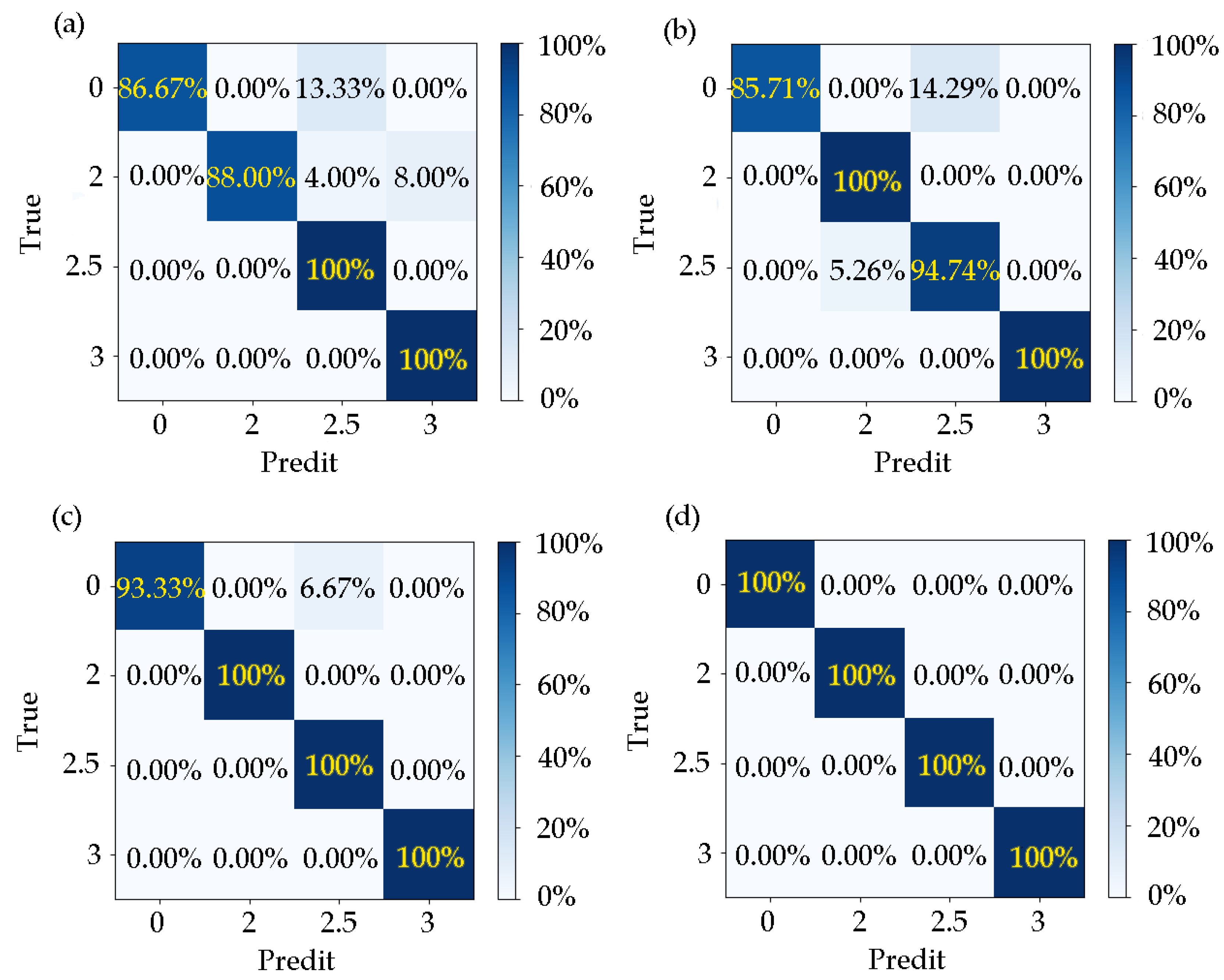
When the training set accounted for 50–90% of the training set, the model’s $accuracy$ for the corresponding test results was 93.75%, 95.31%, 97.92%, 100%, and 100%. It can be seen that the trained model had a good effect on the recognition accuracy of different disease categories.

In the case of different proportions of training samples, $P_{class}$ and $R_{class}$ are shown in

Table 2. The precision of the model.

Training Samples	Class
	P0	P2	P2.5	P3
50%	100.00%	100.00%	85.71%	91.67%
60%	85.71%	92.86%	90.00%	100.00%
70%	93.33%	100.00%	91.67%	100.00%
80%	100.00%	100.00%	100.00%	100.00%
90%	100.00%	100.00%	100.00%	100.00%

and

Table 3. The recall rate of the model.

Training Samples	Class
	R0	R2	R2.5	R3
50%	86.67%	88.00%	100.00%	100.00%
60%	85.71%	100.00%	94.74%	100.00%
70%	93.33%	100.00%	100.00%	100.00%
80%	100.00%	100.00%	100.00%	100.00%
90%	100.00%	100.00%	100.00%	100.00%

and the confusion matrix is shown in Figure 7.

The results for the inter-class precision and recall ratio when the training set samples accounted for 50%, 60%, 70%, 80%, and 90% are shown in

Table 4. Inter-class precision and recall of Co as positive.

Training Samples	Positive = 0
	P0–2	R0–2	P0–2.5	R0–2.5	P0–3	R0–3
50%	100.00%	100.00%	100.00%	86.67%	100.00%	100.00%
60%	100.00%	100.00%	100.00%	85.72%	100.00%	100.00%
70%	100.00%	100.00%	100.00%	93.33%	100.00%	100.00%
80%	100.00%	100.00%	100.00%	100.00%	100.00%	100.00%
90%	100.00%	100.00%	100.00%	100.00%	100.00%	100.00%

,

Table 5. Inter-class precision and recall of HY = 2 as positive.

Training Samples	Positive = 2
	P2–0	R2–0	P2–2.5	R2–2.5	P2–3	R2–3
50%	100.00%	100.00%	100.00%	95.65%	100.00%	91.67%
60%	100.00%	100.00%	92.86%	100.00%	100.00%	100.00%
70%	100.00%	100.00%	100.00%	100.00%	100.00%	100.00%
80%	100.00%	100.00%	100.00%	100.00%	100.00%	100.00%
90%	100.00%	100.00%	100.00%	100.00%	100.00%	100.00%

,

Table 6. Inter-class precision and recall of HY = 2.5 as positive.

Training Samples	Positive = 2.5
	P2.5–0	R2.5–0	P2.5–2	R2.5–2	P2.5–3	R2.5–3
50%	90.00%	100.00%	94.74%	100.00%	100.00%	100.00%
60%	90.00%	100.00%	100.00%	100.00%	100.00%	100.00%
70%	91.67%	100.00%	100.00%	100.00%	100.00%	100.00%
80%	100.00%	100.00%	100.00%	100.00%	100.00%	100.00%
90%	100.00%	100.00%	100.00%	100.00%	100.00%	100.00%

and

Table 7. Inter-class precision and recall of HY = 3 as positive.

Training Samples	Positive = 3
	P3–0	R3–0	P3–2	R3–2	P3–2.5	R3–2.5
50%	100.00%	100.00%	91.67%	100.00%	100.00%	100.00%
60%	100.00%	100.00%	100.00%	100.00%	100.00%	100.00%
70%	100.00%	100.00%	100.00%	100.00%	100.00%	100.00%
80%	100.00%	100.00%	100.00%	100.00%	100.00%	100.00%
90%	100.00%	100.00%	100.00%	100.00%	100.00%	100.00%

.

The data showed that the model did not misjudge patients as normal. When the proportion of training samples was 50%, there were cases in which the normal and disease grade 2 were misjudged as grade 2.5, and grade 2 was mistakenly judged as grade 3. When the proportion of training samples was 40%, there were cases in which the disease grade of 2.5 was misjudged as level 2, and the normal level was wrongly judged as level 2.5. When the proportion of training samples was 30%, normal people were misjudged as the disease grade of 2.5. When the training samples accounted for 20% and 10%, there was no misjudgment. It can be seen that when the proportion of training samples increased, the learners acquired more information, which made the effect of the model gradually better.

3.2. Impact of Processing Strategies

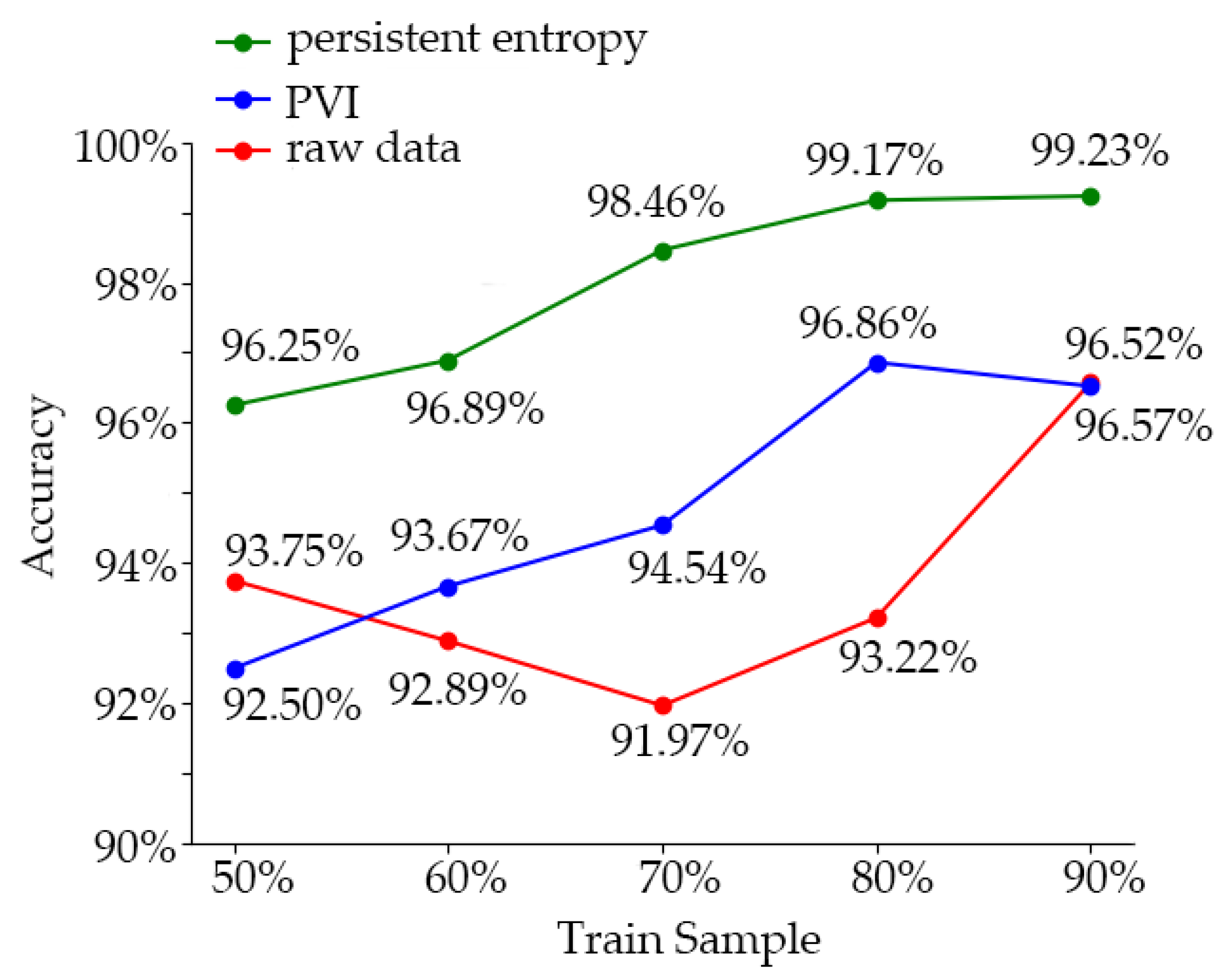
In order to analyze the effect of the sample data-processing method used in this experiment, we used the dataset without processing and the dataset using only the variable-importance processing to train the learner. The training accuracy of the model was compared with the effect of the method used in this experiment. The training accuracy comparison results of the three groups of models are shown in Figure 8. And the comparison to other researches and summarized is shown in

Table 8. Comparison with other methods.

	Yan Yan et al. [26]	Enas Abdulhay et al. [22]	Aite Zhao et al. [19]	Wei Zeng et al. [20]	Tunç Aşuroğlu et al. [23]	Present method
Accuracy	87.10%	94.14%	98.70%	98.80%	99.00%	99.23%

From the comparison results, we can see that the training accuracy of the model trained by the combination of variable-importance processing and TDA persistent entropy was up to 99.23% (the training samples accounted for 90%). The training accuracy of the model trained with the dataset treated by the importance of variables did not increase with the increase of the proportion of training samples (96.86%, 80%; 96.52%, 90%), and maintained at this level. Without data processing, the training accuracy of the model trained by the learner appeared as a U-shaped curve from high to low and then to high; when the training set accounted for 50% to 90%, the training accuracy was 93.75%, 92.89%, 91.97%, 93.72%, and 96.57%, respectively. The reason for this is that SVM could well fit a small number of samples, while the features of the data without processing were not obvious, and the influence of irrelevant features was greater. As the number of samples increased, more complex information appeared, which reduced the training accuracy. When the number of samples increased further, the learner acquired more information, which made the training accuracy increase. In conclusion, the training effect of SVM in a small sample dataset was excellent, and the irrelevant features could be eliminated by variable-importance processing to avoid overfitting of the training model. Using topology analysis and persistent entropy training could further enhance the discrimination of samples and significantly improved the training accuracy.

4. Discussion and Conclusions

There is always a problem of insufficient samples in the recognition of PD. Similar to other studies of abnormal gait, the number of subjects with different disease grades of PD is usually very limited, and the samples are commonly unbalanced. These factors suggest that the grade recognition of PD is a few-shot learning problem.

In this paper, the common GRF dataset was used, which can show the walking pattern of PD patients well. However, from the point of view of the learning effect, the training accuracy curve of the model trained by GRF data showed a U-shape with an increase of the number of samples. The reason for this phenomenon is that the feature discrimination of untreated GRF data was not significant, and contained many irrelevant features/interferences. When the number of samples increased, the learner could not fit the new irrelevant information well, which led to the reduction of training accuracy. This indicates that the GRF data contained too much disturbing information. In another way, some characteristics did not change much among classes.

To solve this problem, we processed the original GRF sample data. The GRF sample data was first divided according to the gait cycle. Considering the existence of minority classes (such as the abnormal gait class), if the time span of GRF data used to calculate gait characteristics was too long, it could cause the loss of key information, and it would not be able to clearly characterize the abnormal gait problem. After the data partition, GRF was used to calculate potential gait features that may affect the classification of the disease grade. For the selection of gait features, we referred to the relevant research and the previous research [22,41], and selected a series of gait features that could be calculated from GRF data for further analysis. After the potential gait features were obtained, we measured the importance of gait features.

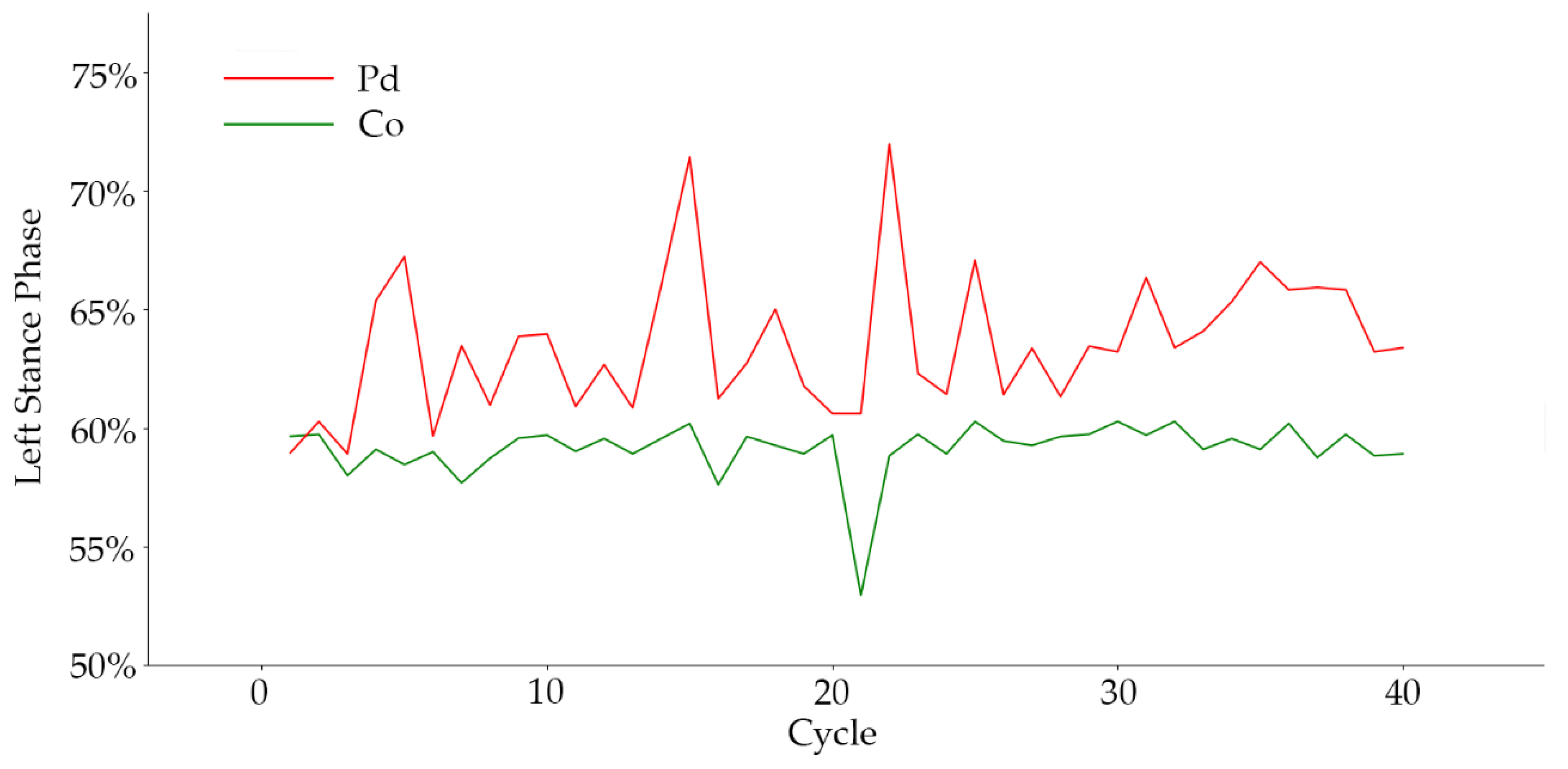
From the experiment results, we observed that the aggravation of PD was directly reflected in walking speed. When the severity of the disease worsened, serious gait disorders hindered the patient from normal speed walking, resulting in a slow movement. This conclusion was strongly supported by the experiments. In addition, walking speed was observed to also affect the stride time of patients, which is also reflected in the results. In other gait features with significant influence, we found that the proportion of gait phase in the classification of disease grade had a high degree of differentiation. There were great differences in the proportion of support-phase and swing-phase time in patients with different disease grades, which also reflects the walking mode of patients with different severity levels. When abnormal gaits such as freezing gait and panic gait occurred, the proportion of gait phase changed significantly. In frozen gait, the proportion of support phase increased significantly. The frequency of the abnormal gait increased significantly when the disease grade was aggravated, and the change of the proportion of gait phase was more clear. For instance, the left-foot gait-phase ratio of PD patients to control subjects is shown in Figure 9.

At the same time, we demonstrated that the RMS of coordinates CoP velocity, CoP efficiency, and sample entropy have significant discrimination in the Y-axis direction. This result indicated that the component of the gait characteristic in the walking direction could significantly influence the classification of disease grade of PD. In addition, according to the importance of the left and right directions of each feature and the importance of CSIP coordinates, we found that there was no significant difference in gait symmetry among PD patients, so this symmetry could not be used as a basis for distinguishing disease grades; that is to say, the abnormal gait pattern of PD was not found in only one limb.

Considering the complexity of the human body, we analyzed the gait features. The results showed that the persistent entropy model was better than the model without topology data analysis. Although we could get good results by measuring the importance of variables, the training accuracy reached the peak when the proportion of training samples reached 80%. Increasing the number of training samples could not improve the training accuracy. This indicates that the effect of only using gait features to distinguish different PD grades encountered a bottleneck. When the persistent entropy was used as the training sample, the training accuracy of the learner broke through this bottleneck and reached 99.23%. The results showed that the TDA method could further extract the differences between gait features of different disease grades, and improved the discrimination among classes. This was due to the strong nonlinearity and complexity of human walking, and the SVM we used was essentially a linear classifier. The TDA method could map the gait feature data to the high-dimensional space and mine the sample features at a deeper level, which made the sample discrimination increase. Therefore, it was suitable for solving few-shot machine-learning problems related to human gait.

In addition, the training cost of samples processed by different methods is also different. The method of persistent entropy can be simplified to represent a class of gait features with only three numbers, which greatly reduces the dimension of the sample and significantly reduces the computation load during training.

In the problem of sample balancing, persistent entropy is used to strengthen the discrimination between different classes of samples, which makes the distance between different categories further. This avoids the blindness of the SMOTE algorithm in neighbor selection to a certain extent, and makes the synthesized samples achieve a better training effect. According to the misclassification of severity levels, there are some cases in which normal people are recognized as patients, or low-level cases are identified as high-level cases. This is because when there are too few training samples, the walking speed becomes the most important feature. When the walking speed of the older normal or mild patients is too slow, the learner will mistakenly classify them as a serious manifestation of the disease, resulting in misclassification. When the number of training samples increases, this kind of misclassification can be improved.

In summary, this paper proposed a few-shot learning method based on the measurement of permutation-variable importance and topological-imprint persistent entropy. The GRF was used as the basic data, Borderline-SMOTE was used as sample balancing method, and SVM was used as a classifier to identify the grade of PD. The proposed method achieved better results than when using original data. At the same time, the results of our study also indicated the leading factors of the differences among disease grades, which is valuable in further understanding the differential performance of different PD grades, revealing the walking characteristics of PD patients, and guiding the targeted health care.