Model-Free High Order Sliding Mode Control with Finite-Time Tracking for Unmanned Underwater Vehicles

Abstract

Several strategies to deal with the trajectory tracking problem of Unmanned Underwater Vehicles are encountered, from traditional controllers such as Proportional Integral Derivative (PID) or Lyapunov-based, to backstepping, sliding mode, and neural network approaches. However, most of them are model-based controllers where it is imperative to have an accurate knowledge of the vehicle hydrodynamic parameters. Despite some sliding mode and neural network-based controllers are reported as model-free, just a few of them consider a solution with finite-time convergence, which brings strong robustness and fast convergence compared with asymptotic or exponential solutions and it can also help to reduce the power consumption of the vehicle thrusters. This work aims to implement a model-free high-order sliding-mode controller and synthesize it with a time-base generator to achieve finite-time convergence. The time-base was included by parametrizing the control gain at the sliding surface. Numerical simulations validated the finite-time convergence of the controller for different time-bases even in the presence of high ocean currents. The performance of the obtained solution was also evaluated by the Root Mean Square (RMS) value of the control coefficients computed for the thrusters, as a parameter to measure the power consumption of the vehicle when following a trajectory. Computational results showed a reduction of up to 50% in the power consumption from the thrusters when compared with other solutions.

1. Introduction

Unmanned Underwater Vehicles (UUVs) are used in multiple tasks such as ship’s hull inspection [1], ecological surveys [2,3], underwater inspection and mapping [4], among others. The use of UUVs avoid risks for human divers and reduce operational costs. In addition, they can perform some tasks that cannot be done by humans in an underwater environment. The motion of these vehicles can be remotely operated (ROVs) or autonomous (AUVs). For ROVs, there is a human pilot that commands the vehicle’s movements and actions, usually through a tether. Human presence makes complex exploration and intervention tasks possible since humans can react to changes in the mission plan caused by the unpredictable nature of the underwater environments. However, certain operations such as high precision navigation require some form of autonomy from the vehicle. That is a complex task to achieve and one of the main problems for AUVs [5] since their six Degree of Freedom (DOF) dynamics is highly non-linear and, therefore, difficult to control [6]. Motion control of a UUV has different goals such as waypoint tracking, path following, and trajectory tracking [7]. For waypoint tracking, the controller should guide the vehicle from a starting position to the desired destination throughout a set of pre-defined waypoints. For path following, the aim is that the vehicle accurately follows the desired path in terms of a geometric description while the trajectory tracking problem requires the vehicle to converge to a desired time-parametrized trajectory. For trajectory tracking, convergence can be either asymptotic, exponential, or in finite-time.

Several control strategies have been applied in the past to achieve high precision trajectory tracking. The Proportional Integral Derivative (PID) control is one of the most employed control strategies for UUVs due to their simple structure. They work well for systems where it is possible to control all outputs through the inputs—meaning they are not underactuated—and are widely used for heading, depth, and surge control [8]. However, one limitation for PID controllers is that they are tuned to deal with specific conditions and, if those conditions change, the performance will be affected. In addition, PID controllers do not consider nonlinearities, which will eventually deteriorate the controller performance. Some other strategies are used with the PID controller to compensate some of the uncertainties faced in the underwater environment. Dong et al. [9] designed a fuzzy rules-based strategy to tune a PID depth controller. Experiments were carried out to test the controller, showing a depth control accuracy of up to 3 cm. Yang et al. [10] adopted a cascade PID structure to deal with horizontal displacements in the heading control. Experimental results showed better performance when compared with a traditional PID controller since oscillations were reduced and even eliminated when controlling the heading of the ROV. Zhang et al. [11] used Particle Swarm Optimization (PSO) to optimize the parameters of a PID controller for horizontal displacements. Simulation results showed better performance than a PID controller, but weaker compared with a fuzzy controller. Hernández-Alvarado et al. [12] proposed a Neural Network (NN) based self-tuning PID controller where the NN automatically estimates a suitable set of gains for the PID controller to achieve system stability. The controller was validated with numerical simulations and experimentation, showing better performance when subject to unknown disturbances and over 3% of energy-saving against a traditional PID controller.

Backstepping Control (BC) is a model-based nonlinear controller that is commonly used for trajectory tracking of UUVs. It is based on the Lyapunov theory [13] and works by sectioning the dynamic system of the vehicle into subsystems, so the controller begins with a known stable system and then iterates to obtain proper controllers for the rest of the subsystems. Yan et al. [14] applied backstepping control to the trajectory tracking of an AUV to a docking station. Simulations of their controller showed that all tracking errors converge to a small neighborhood of the origin. Zhou et al. [15] proposed a solution for underactuated AUVs tracking using a combination of a Neural Network (NN) algorithm and a backstepping sliding mode controller. Simulations showed a smooth tracking of the desired three-dimensional trajectory. Yan et al. [13] proposed a backstepping sliding mode controller with fuzzy switching gain. Simulation results showed that the controller designed can guarantee that the UUV accurately track the desired path in the presence of time-varying interference and effectively eliminate the chattering in the traditional Sliding Mode Control (SMC) method.

SMC is another typical approach for trajectory tracking of UUVs. It has been extensively applied due to its simple form, robustness, and tolerance to model uncertainty. However, SMC has the problem of chattering. For UUV control, the chattering causes high-frequency changes in the speed of the thrusters, which leads to high energy consumption, increase friction, and thruster damage [16]. Ramezani-al et al. [17] proposed an SMC with adaptative gain. In their controller, a continuous term is used instead of a discrete traditional sign function, a large gain for the sliding mode is applied to satisfy the reaching condition, as well as a small gain for the sliding mode to avoid the chattering phenomena. Simulation results showed the controller proposed can decrease the amplitude of chattering in the control signal and increase the convergence rate to the desired trajectory. Lv et al. [18] proposed a fault-tolerant control method integrated with thrust allocation based on the sliding mode theory. Experimental results showed a reduction of up to 94% of the steady error compared with a conventional SMC. García-Valdovinos et al. [19] proposed a 2nd order SMC combined with a backpropagation NN control scheme for UUVs to deal with external disturbances and parameter variations. Experimental results showed that the controller was able to reduce the position error to zero in a robust way while the online adjustments of the weights in the NN compensated for the variations in the vehicle hydrodynamics and perturbations.

Despite the numerous approaches for trajectory tracking of UUVs encountered, just a few of them have considered a finite-time convergence. Finite-time control is an effective control strategy with strong robustness and fast convergence. It has many advantages such as faster convergence time, higher accuracy, and better anti-disturbance capability [20]. Yan et al. [21] adopted the globally finite-time tracking control strategy, along with a PID-SMC model-based controller, to track a predefined trajectory for a UUV. Simulations showed that the control laws can achieve strongly robust and preferably control performance for the horizontal trajectory tracking control in the presence of parameter perturbation and unknown currents. Their work was extended to three-dimensional trajectory tracking by Yu et al. [22]. Simulation results show that the vehicle can converge to the trajectory and remain in a small neighborhood even in the presence of ocean currents, wherein a small fluctuation in the tracking errors is observed. Chu et al. [23] proposed a local recurrent NN for finite-time trajectory tracking of ROVs with an unknown dynamical model. The authors designed a state observer based on sliding-mode to estimate those variables that cannot be measured by the ROV and achieved finite-time convergence with the adaptative controller proposed. Qiao et al. [24] proposed two control schemes based on sliding mode to the tracking control of UUVs in presence of uncertainties and disturbances: an adaptive integral terminal sliding mode control and an adaptive fast integral terminal sliding mode control. Each controller is composed of a kinematic and a dynamic controller, where the kinematic can achieve local finite-time convergence of the tracking error to zero. Guerrero et al. [25] proposed an adaptative high order SMC with finite-time convergence for an AUV. The authors validated the proposed controller with real experiments for depth and yaw trajectories, considering parametric uncertainties and external disturbances.

Finite-time tracking controllers have been widely and successfully used to control fully actuated robot arms [26,27], but little research has been done for underactuated unmanned underwater vehicles (UUVs), whose particular nonlinear dynamics have other challenges, for instance, the hydrodynamics effects inherent to the vehicle’s geometry and water density. Considering the advantages of a controller with finite-time convergence, and that most of the controllers designed to achieve that for trajectory tracking in UUVs navigation are model-based 1st order SMC, this paper presents the formulation and validation of a model-free 2nd order SMC based on a Time Base Generator (TBG) that guarantees finite-time three-dimensional trajectory tracking of underactuated UUVs subject to ocean currents. The resulting control law does neither depend on the hydrodynamics nor other parameters of the vehicle; therefore, it is considered as a model-free controller. In addition, formulation of the control law of this 2nd order SMC eliminates the chattering effect which is common in conventional 1st order SMC [28,29]. To achieve finite-time convergence of the tracking errors of three-dimensional trajectories, the 2nd order SMC is parametrized by a TBG which allows the user to set an arbitrary base-time in which the vehicle will meet the desired trajectory. The performance of the proposed controller is evaluated by numerical simulations including the effects of external disturbances. All this is structured in this paper as: Section 2 describes the BlueROV2 UUV and its dynamic model, as well as the proposed control scheme including the TBG. Section 3 describes the method and parameters used to validate the proposed controller. Section 4 shows the results of the testing and validation, and Section 5 contains the concluding remarks.

2. Materials and Methods

2.1. Unmanned Underwater Vehicle Model

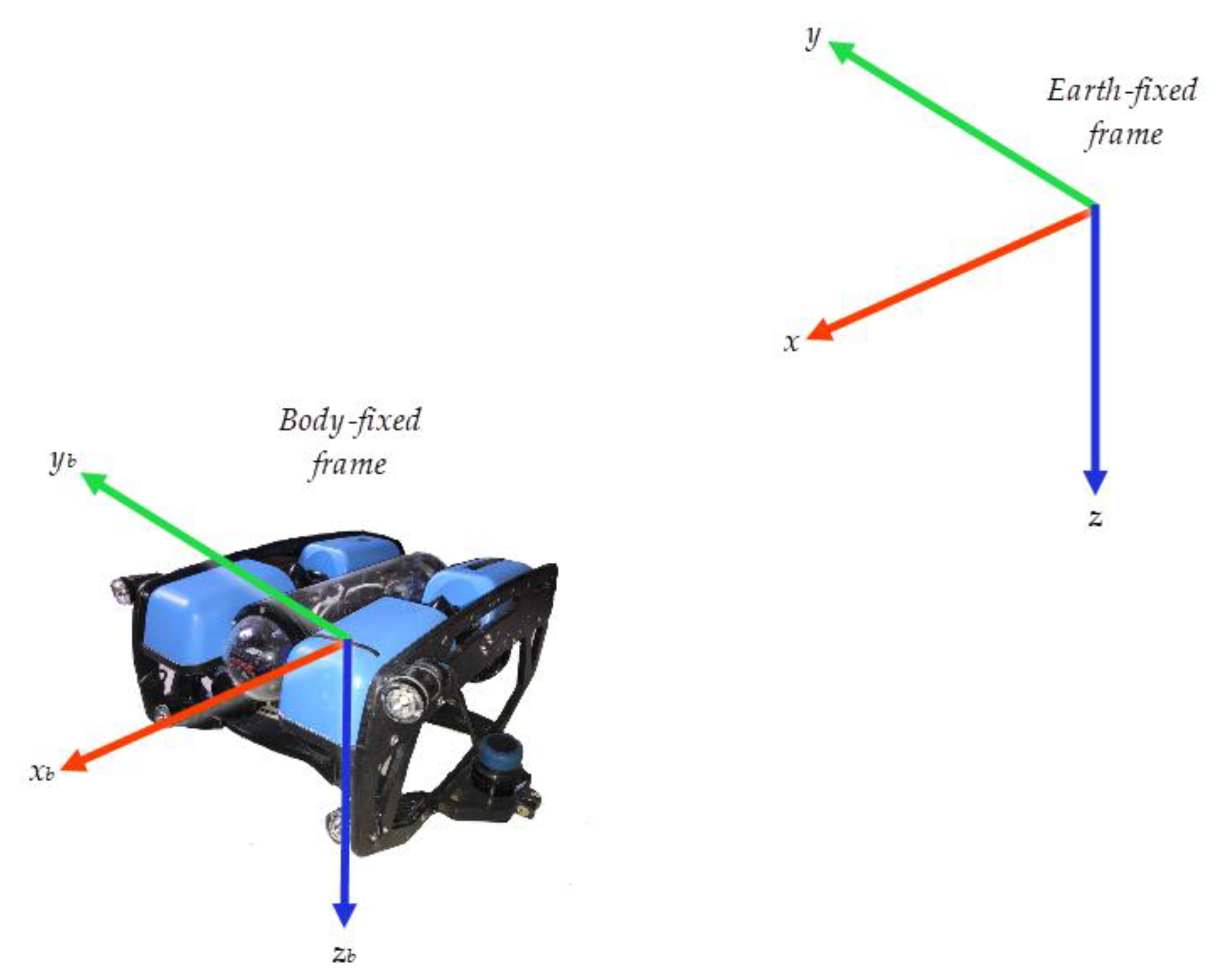
2.1.1. Kinematic Model

As described by Fossen [30], two reference frames are needed to build the mathematical model that represents the underwater vehicle: one referenced to the earth (labeled as Earth-fixed frame) and the other referenced to the vehicle (labeled as body-fixed frame). The orthonormal axes are denoted by $x,y,z$ for the Earth-fixed frame, and by $x_b,y_b,z_b$for the body-fixed frame. These reference frames are shown in Figure 1.

The Society of Naval Architects and Marine Engineers (SNAME) has a convention to express the position and orientation of vehicles, and the forces and moments applied to them. The SNAME nomenclature for position, velocity, and forces in underwater vehicles [30] is presented in

Table 1. Notation for underwater vehicle’s movements, positions, velocities, and forces.

Movement	Name	Position	Velocity	Force/Moment
X translation	Surge	x	u	X
Y translation	Sway	y	v	Y
Z translation	Heave	z	w	Z
X rotation	Roll	φ	p	K
Y rotation	Pitch	θ	q	M
Z rotation	Yaw	ψ	r	N

.

The position of the vehicle with respect to the Earth-fixed frame $\eta$ and its velocity with respect the body-fixed frame $\nu$ can be represented as

$$\eta ={\left(x,y,z,\phi ,\theta ,\psi \right)}^T,$$

(1)

$$\nu ={\left(u,v,w,p,q,r\right)}^T,$$

(2)

The forces and moments of the vehicle with respect to the body-fixed frame are described as

$$\tau ={\left(X,Y,Z,K,M,N\right)}^T,$$

(3)

2.1.2. Hydrodynamic Model

The hydrodynamic model of a UUV can be described by Newton–Euler equations [30] as

$$M\dot{\nu }+C\left(\nu \right)\nu +D\left(\nu \right)\nu +g\left(\eta \right)= \tau +\omega ,$$

(4)

$$\tau = B_t{u}_t,$$

(5)

where

• M ∈ℝ^6×6 is the inertial and added mass matrix,
• C ∈ℝ^6×6 is the rigid body and added mass centripetal and Coriolis matrix,
• D ∈ℝ^6×6 is the hydrodynamic damping matrix,
• g ∈ℝ^6×1 is the restitution forces vector,
• $B_t$ ∈ℝ^6×6 is the thruster allocation matrix,
• $u_t$ ∈ℝ^6×1 is a vector containing the force generated by the thrusters, and
• $\omega$ ∈ℝ^6×1 represents environmental disturbances.

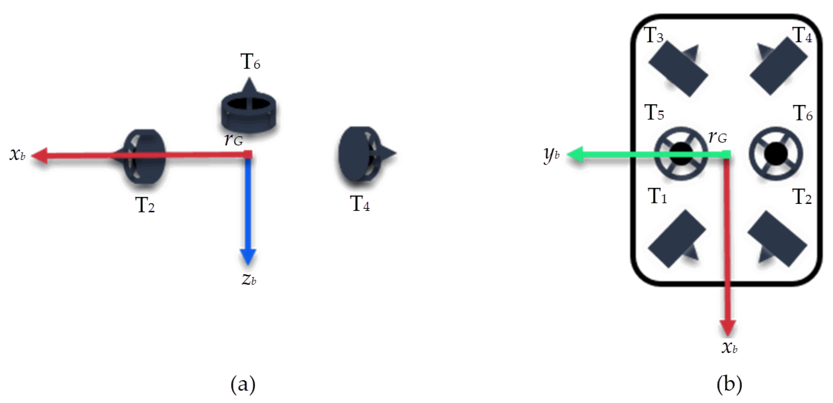
2.1.3. BlueROV2 Model

The vehicle considered for the simulations in this work was the BlueROV2 from Blue Robotics^®. It has the six-thruster vectored configuration that can be seen in Figure 2.

Matrices and vectors involved in the vehicle’s hydrodynamics contain numerous unknown parameters, making it infeasible to estimate. Nevertheless, there are some assumptions and considerations that can be made because of the BlueROV2 geometry and operation, resulting in a considerable reduction of unknown parameters. These conditions are listed below:

• Since BlueROV2 operates at relatively low speeds (i.e., less than 2 m/s), lift forces can be neglected.
• BlueROV2 is assumed to have port-starboard symmetry and fore-aft symmetry, and the center of gravity (CG) is in the symmetry planes.
• BlueROV2 is assumed to operate below the wave-affected zone. As a result, disturbances of waves $\omega$ on the vehicle are negligible.
• The thruster allocation of BlueROV2 does not permit active control of the pitch orientation q. However, the motion around this axis is considered self-regulated due to the vehicle buoyant restoring moments, resulting in the following reduced system

$$\nu ={\left(u,v,w,p,0,r\right)}^T,$$

(6)

Considering the reduced system detailed before, the physical and hydrodynamic parameters of BlueROV2 are summarized in

Table 2. BlueROV2 parameters.

Parameters	Symbol	Value	Unit
Mass	m	10	kg
Buoyancy	B	100.06	N
Weight	W	98.1	N
Center of gravity	$r_G=\left(x_g,y_g,z_g\right)$	$r_G=\left(0,0,0\right)$	m
Center of buoyancy	$r_B=\left(x_b,y_b,z_b\right)$	$r_B=\left(0,0,0.02\right)$	m
Inertia moment	I = diagonal ($I_x,I_y,I_z$)	I = diagonal (0.16$,0.16,0.16$)	$\mathrm{kg}·{\mathrm{m}}^2$
Added mass parameters	$X_{\dot{u}}$	−5.5	kg
	$Y_{\dot{v}}$	−12.7	kg
	$Z_{\dot{w}}$	−14.57	kg
	$K_{\dot{p}}$	−0.12	$\mathrm{kg}·\frac{{\mathrm{m}}^2}{\mathrm{rad}}$
	$M_{\dot{q}}$	−0.12	$\mathrm{kg}·\frac{{\mathrm{m}}^2}{\mathrm{rad}}$
	$N_{\dot{r}}$	−0.12	$\mathrm{kg}·\frac{{\mathrm{m}}^2}{\mathrm{rad}}$
Linear Damping parameters	$X_u$	−4.03	$\mathrm{N}·\frac{\mathrm{s}}{\mathrm{m}}$
	$Y_v$	−6.22	$\mathrm{N}·\frac{\mathrm{s}}{\mathrm{m}}$
	$Z_w$	−5.18	$\mathrm{N}·\frac{\mathrm{s}}{\mathrm{m}}$
	$K_p$	−0.07	$\mathrm{N}·\frac{\mathrm{s}}{\mathrm{rad}}$
	$M_q$	−0.07	$\mathrm{N}·\frac{\mathrm{s}}{\mathrm{rad}}$
	$N_r$	−0.07	$\mathrm{N}·\frac{\mathrm{s}}{\mathrm{rad}}$
Quadratic Damping parameters	$X_{u\left|u\right|}$	−18.18	$\mathrm{N}·\frac{{\mathrm{s}}^2}{{\mathrm{m}}^2}$
	$Y_{v\left|v\right|}$	−21.66	$\mathrm{N}·\frac{{\mathrm{s}}^2}{{\mathrm{m}}^2}$
	$Z_{w\left|w\right|}$	−36.99	$\mathrm{N}·\frac{{\mathrm{s}}^2}{{\mathrm{m}}^2}$
	$K_{p\left|p\right|}$	−1.55	$\mathrm{N}·\frac{{\mathrm{s}}^2}{{\mathrm{rad}}^2}$
	$M_{q\left|q\right|}$	−1.55	$\mathrm{N}·\frac{{\mathrm{s}}^2}{{\mathrm{rad}}^2}$
	$N_{r\left|r\right|}$	−1.55	$\mathrm{N}·\frac{{\mathrm{s}}^2}{{\mathrm{rad}}^2}$

as identified in [31,32,33].

The matrices that comprise the hydrodynamical model in Equation (4) are considered as defined in [30].

Considering the thruster distribution in the BlueROV2, the thruster allocation matrix is assembled as

$$B_t=\left[\begin{array}{cccccc}0.7071& 0.7071& -0.7071& -0.7071& 0& 0\\ -0.7071& 0.7071& -0.7071& 0.7071& 0& 0\\ 0& 0& 0& 0& -1& -1\\ 0& 0& 0& 0& 0.115& -0.115\\ 0& 0& 0& 0& 0& 0\\ -0.1773& 0.1773& -0.1773& 0.1773& 0& 0\end{array}\right]$$

(7)

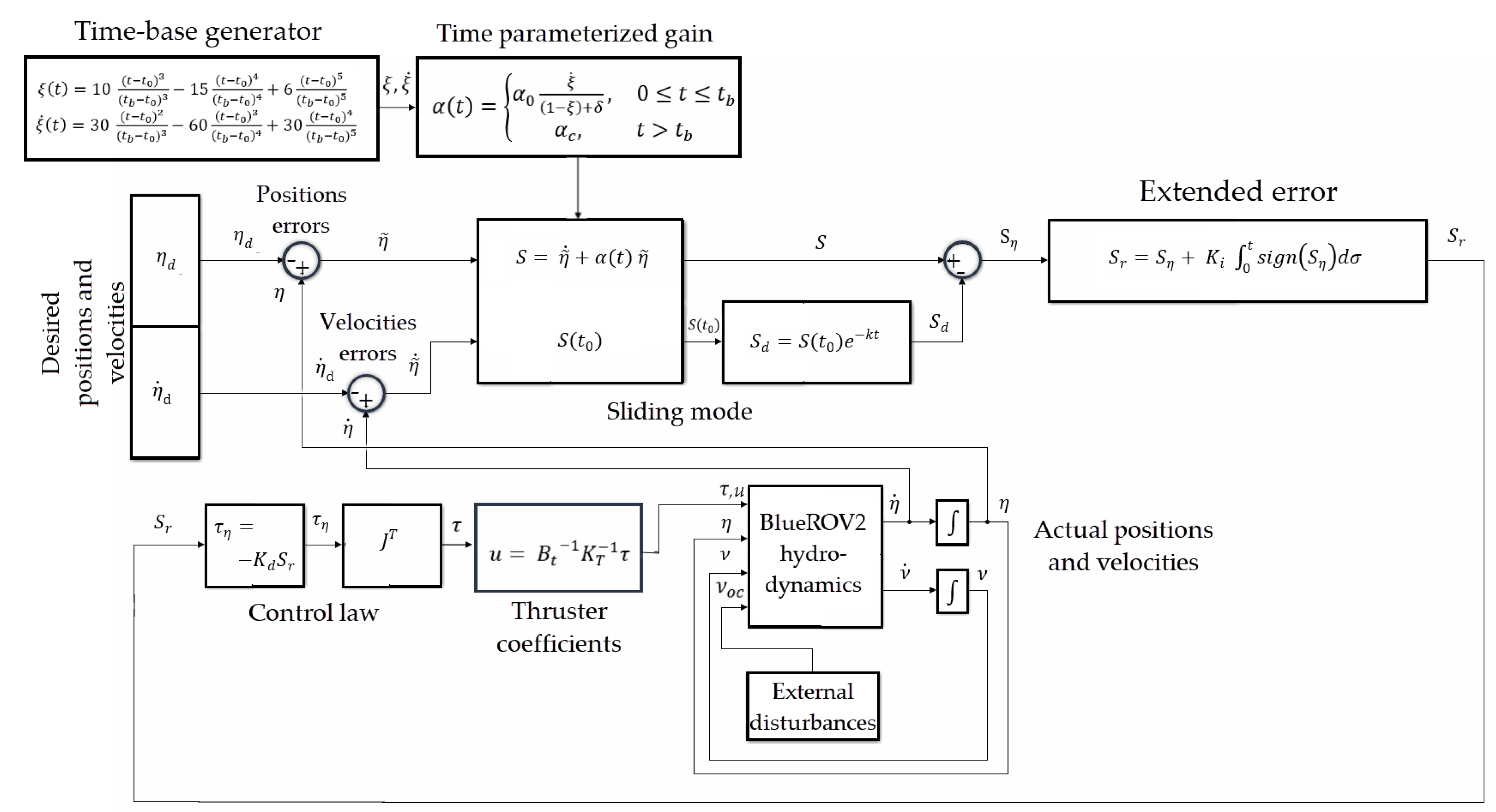
2.2. Model-Free High-Order SMC with Finite-Time Convergence

The dynamics of the UUV (Equation (4)) can be expressed in the Earth-fixed frame applying the following kinematic transformations [30]

$$\dot{\eta }=J\left({\eta }_2\right) \nu \leftrightarrow \nu = J^{-1}\left({\eta }_2\right) \dot{\eta },$$

(8)

$$\ddot{\eta }=J\left({\eta }_2\right) \dot{\nu }+ \dot{J}\left({\eta }_2\right) \nu \leftrightarrow \dot{\nu }= J^{-1}\left({\eta }_2\right) \left[\ddot{\eta }- J\left({\eta }_2\right) \nu \right],$$

(9)

where the transformation matrix $J\left({\eta }_2\right)$ is defined as

$$J\left({\eta }_2\right)= \left[\begin{array}{cc}{J}_1\left({\eta }_2\right) & 0_{3\times 3}\\ 0_{3\times 3}& J_2\left({\eta }_2\right) \end{array}\right],$$

(10)

with

$$\begin{gathered} J_1\left({\eta }_2\right)=\left[\begin{array}{ccc}{c}_{\mathsf{\psi }}{c}_{\mathsf{\theta }}& -s_{\mathsf{\psi }}{c}_{\varphi }+s_{\varphi }{s}_{\mathsf{\theta }}{c}_{\mathsf{\psi }}& s_{\mathsf{\psi }}{s}_{\varphi }+s_{\mathsf{\theta }}{c}_{\mathsf{\psi }}{c}_{\varphi }\\ s_{\mathsf{\psi }}{c}_{\mathsf{\theta }}& c_{\mathsf{\psi }}{c}_{\varphi }+s_{\varphi }{s}_{\mathsf{\theta }}{s}_{\mathsf{\psi }}& -c_{\mathsf{\psi }}{s}_{\varphi }+s_{\mathsf{\theta }}{s}_{\mathsf{\psi }}{c}_{\varphi }\\ -s_{\mathsf{\theta }}& s_{\varphi }{c}_{\mathsf{\theta }}& c_{\varphi }{c}_{\mathsf{\theta }}\end{array}\right], \\ {J}_s\left({\eta }_2\right)= \left[\begin{array}{ccc}1& s_{\varphi }{t}_{\mathsf{\theta }}& c_{\varphi }{t}_{\mathsf{\theta }}\\ 0& c_{\varphi }& -s_{\varphi }\\ 0& s_{\varphi }/c_{\mathsf{\theta }}& c_{\varphi }/c_{\mathsf{\theta }}\end{array}\right], \mathrm{and} \end{gathered}$$

$${\eta }_2={\left[\varphi ,\theta ,\psi \right]}^T,$$

where $c_{angle}=cos\left(angle\right)$, $s_{angle}=sin\left(angle\right)$, and $t_{angle }=tan\left(angle\right)$.

After some mathematical manipulation, the resulting expression is

$$M_{\eta }\left(\eta \right)\ddot{\eta }+C_{\eta }\left(\nu ,\eta \right)\dot{\eta }+D_{\eta }\left(\nu ,\eta \right)\dot{\eta }+g_{\eta }\left(\eta \right)= {\tau }_{\eta },$$

(11)

where

$$M_{\eta }\left(\eta \right)= J^{-T}\left(\eta \right)M{J}^{-1}\left(\eta \right),$$

$$C_{\eta }\left(\nu ,\eta \right)= J^{-T}\left(\eta \right)[C\left(\nu \right)-M{J}^{-1}\left(\eta \right)\dot{J}\left(\eta \right)]J^{-1}\left(\eta \right),$$

$$D_{\eta }\left(\nu ,\eta \right)= J^{-T}\left(\eta \right)D\left(\nu \right)J^{-1}\left(\eta \right),$$

$$g_{\eta }\left(\eta \right)= J^{-T}\left(\eta \right)g\left(\eta \right)$$

$${\tau }_{\eta }\left(\eta \right)= J^{-T}\left(\eta \right)\tau$$

(12)

García-Valdovinos et al. [26,27] established that Equation (10) is linearly parametrizable by the product of a regressor $Y\left(\eta ,\dot{\eta },\ddot{\eta }\right)\in {ℝ}^{n \times p}$ composed of known nonlinear functions and a vector $\theta \in {ℝ}^p$containing constant parameters. Then, this parametrization can be rewritten in terms of a nominal reference ${\dot{\eta }}_r$ and its time derivative ${\ddot{\eta }}_r$ as follows

$$M_{\eta }\left(\eta \right){\ddot{\eta }}_r+C_{\eta }\left(\nu ,\eta \right){\dot{\eta }}_r+D_{\eta }\left(\nu ,\eta \right){\dot{\eta }}_r+g_{\eta }\left(\eta \right)= Y\left(\eta ,\dot{\eta },{\dot{\eta }}_r,{\ddot{\eta }}_r\right)\theta ,$$

(13)

Subtracting Equation (12) from both sides of Equation (10) leads to the open-loop error dynamics expression

$$M_{\eta }\left(\eta \right){\dot{S}}_r+C_{\eta }\left(\nu ,\eta \right)S_r+D_{\eta }\left(\nu ,\eta \right)S_r={\tau }_{\eta }- Y\left(\eta ,\dot{\eta },{\dot{\eta }}_r,{\ddot{\eta }}_r\right)\theta ,$$

(14)

where $S_r=\dot{\eta }-{\dot{\eta }}_r$ is known as the extended error.

Now, consider the following nominal reference

$${\dot{\eta }}_r= {\dot{\eta }}_d-\alpha \tilde{\eta }+S_d-K_i{{\displaystyle \int }}_0^{t}sign\left(S_{\eta }\right)d\sigma ,$$

(15)

where $\tilde{\eta }=\eta -{\eta }_d$ represents the tracking error of the position, ${\eta }_d$ is the desired trajectory, $\alpha$ and $K_i$ are diagonal positive definite $n \times n$ gain matrices, $sign\left(x\right)$ stands for the $signum function$ of vector $x$ and

$$S= \dot{\tilde{\eta }}+\alpha \tilde{\eta },$$

(16)

$$S_d=S\left(t_0\right)e^{-\kappa t},$$

(17)

$$S_{\eta }=S-S_d,$$

(18)

with $\kappa >0$. So that the extended error $S_r$ can be rewritten as follows

$$S_r=S_{\eta }+ K_i {{\displaystyle \int }}_0^{t}sign\left(S_{\eta }\right)d\sigma ,$$

(19)

The result is the model-free high-order SMC with the following control law

$${\tau }_{\eta }=-K_d{S}_r,$$

(20)

Notice that the so-called model-free control law does not depend on any parameter, matrix, or vector describing the hydrodynamics of the vehicle, it is defined by a diagonal definite positive $n \times n$ gain matrix $K_d$, and the extended error $S_r$. Furthermore, since the $signum function$ is not used directly but through its integral, the chattering effect common in conventional SMC is not present. A stability analysis of the controller just described can be found in [34] where the existence of the sliding mode was proven.

A TBG will be used to achieve finite-time convergence. A TBG is a scalar time function that provides a smooth transition from 0 to 1, with a duration controllable by a time-base $t_b$. Its derivative provides a bell-shaped speed profile. The TBG implemented in this work was introduced by Parra-Vega [26] and García-Valdovinos [27] for finite-time convergence of a robotic arm. Consider the fifth-order polynomial

$$\xi \left(t\right)=10 \frac{{\left(t-t_0\right)}^3}{{\left(t_b-t_0\right)}^3}-15\frac{{\left(t-t_0\right)}^4}{{\left(t_b-t_0\right)}^4}+6\frac{{\left(t-t_0\right)}^5}{{\left(t_b-t_0\right)}^5},$$

(21)

and its time derivative

$$\dot{\xi }\left(t\right)=30 \frac{{\left(t-t_0\right)}^2}{{\left(t_b-t_0\right)}^3}-60\frac{{\left(t-t_0\right)}^3}{{\left(t_b-t_0\right)}^4}+30\frac{{\left(t-t_0\right)}^4}{{\left(t_b-t_0\right)}^5},$$

(22)

with $t_0$ representing the initial time and subjected to the following conditions: $\xi \left(t_0\right)=\dot{\xi }\left(t_0\right)=\dot{\xi }\left(t_b\right)=0.$The time-base $t_b$ can be chosen arbitrarily and does not depend on the initial condition.

Now, $\xi \left(t\right)$ will be used to parameterize a time-varying gain $\alpha \left(t\right)$ as follows

$$\alpha \left(t\right)=\{\begin{array}{c}{\alpha }_0\frac{\dot{\xi }}{\left(1-\xi \right)+\delta }, 0\le t\le t_b\\ {\alpha }_c, t>t_b\end{array},$$

(23)

with ${\alpha }_0=1+\epsilon , 0<\epsilon \ll 1,$ $0<\delta \ll 1$, and ${\alpha }_c$ > 0.

To achieve finite-time convergence in the trajectory tracking of the BlueROV2, the constant gain $\mathsf{\alpha }$ in Equation (15) is replaced with the time-varying gain $\alpha \left(t\right)$ given by Equation (22). Then, the control law described in Equation (19) is applied. The control scheme is represented in the block diagram depicted in Figure 3.

To obtain the forces needed in the thrusters, ${\tau }_{\eta }$ needs to be converted from the Earth-fixed frame to the body-fixed frame as follows

$$\mathsf{\tau }=J^{-1}\left({\eta }_2\right){\tau }_{\eta },$$

(24)

Then, the control coefficient vector $u$ for the thrusters is computed as

$$u=B_t{}^{-1}{K}_T{}^{-1}\mathsf{\tau }$$

(25)

where $K_T$ is a diagonal matrix containing the maximum force (N) each thruster can produce. Then, the control coefficient vector$u$ is limited to a range of $-1\le u\le 1$ to avoid thruster saturation and to keep the control signal introduced to the model in a range that can be achievable by the thrusters.

3. Validation Method for the Controller

To test and validate the proposed control scheme the hydrodynamics of the BlueROV2—as presented in Section 2.1—was programmed in a simulator developed in MATLAB/Simulink^®. This simulator also considers some external disturbances such as ocean currents.

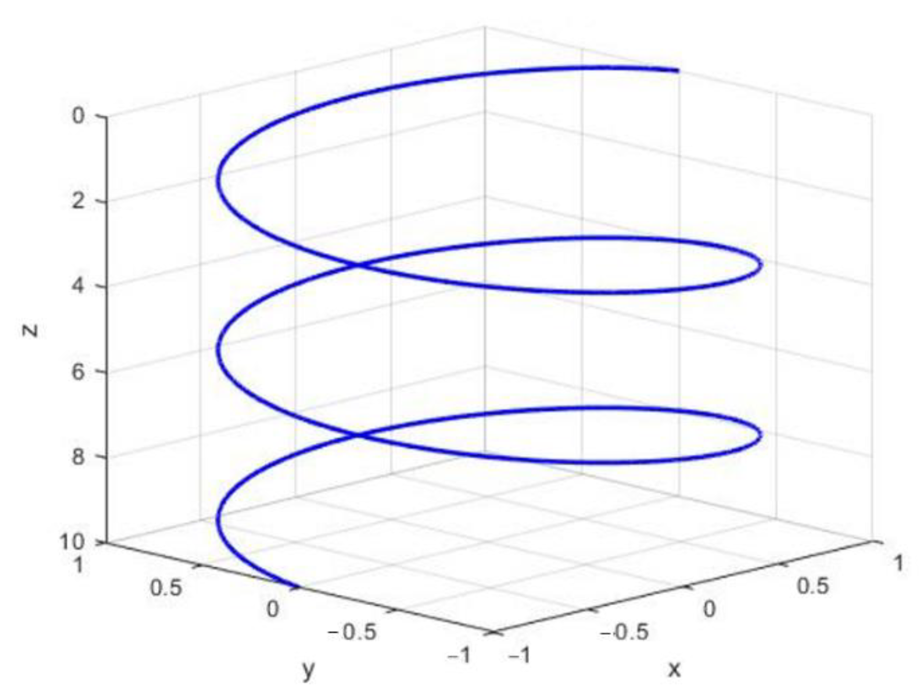
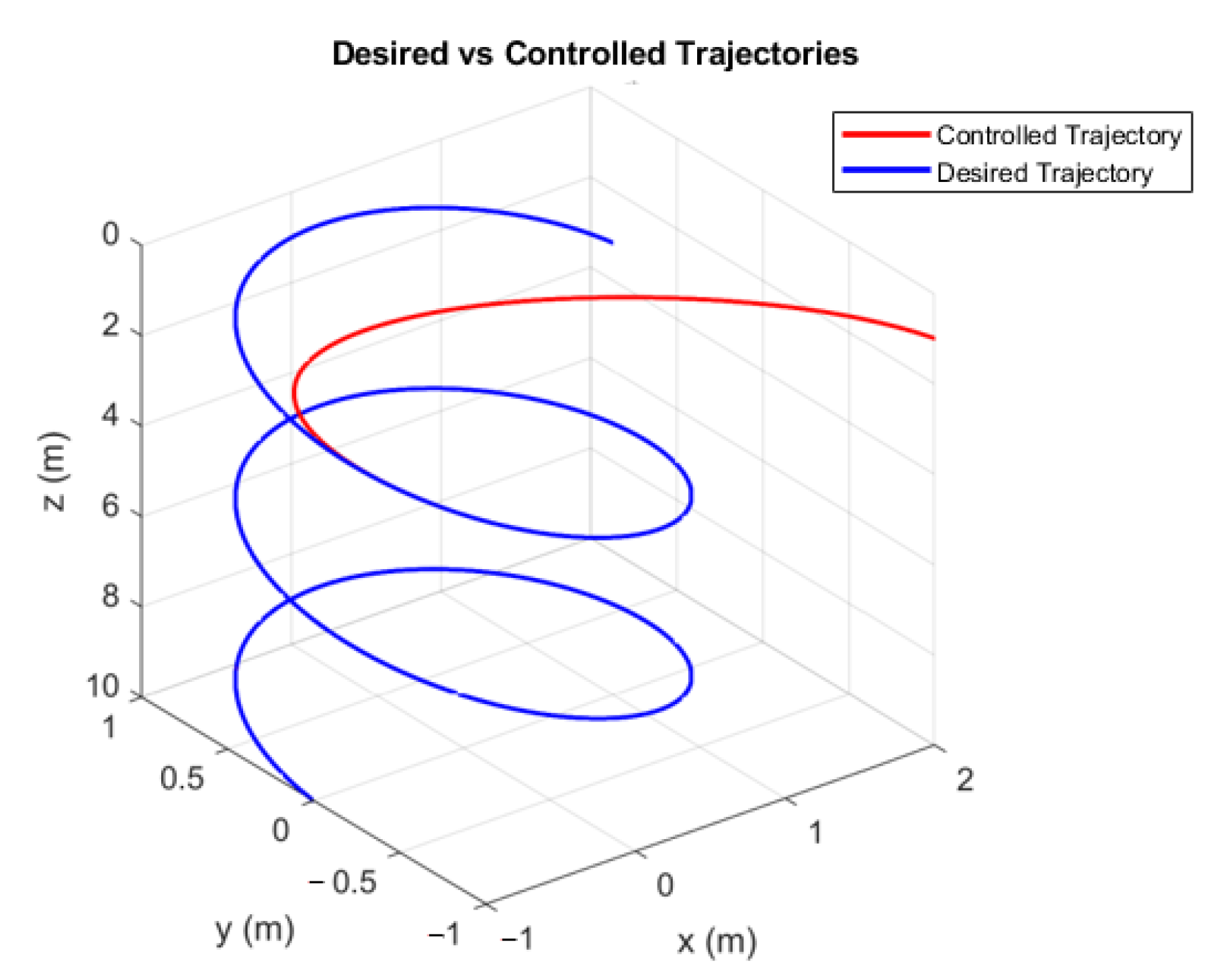
3.1. Parameterized Trajectory of the UUV

A spiral trajectory was selected to be able to control all DOFs of the BlueROV2 ($x,y,z,\phi ,\psi$) while moving simultaneously at surge, sway, heave, and yaw. The desired positions ${\eta }_d$ and velocities ${\dot{\eta }}_{\mathrm{d}}$ are given by the following equations

$${\eta }_d=\left(x_d,y_d,z_d,{\phi }_d,{\psi }_d\right),$$

(26)

where

$$x_d=x_i+Rcos\left(\omega t\right),$$

$$y_d=y_i+R sin\left(\omega t\right),$$

$$z_d=z_i+(z_f-z_i) \frac{t}{t_s},$$

$${\phi }_d=0, \mathrm{and}$$

$${\psi }_d= {\psi }_i+\omega t,$$

$${\dot{\eta }}_d=\left(\dot{x_d},\dot{y_d},\dot{z_d},\dot{{\phi }_d},\dot{{\psi }_d}\right),$$

(27)

where

$${\dot{x}}_d=- \omega Rsin\left(\omega t\right),$$

$${\dot{y}}_d=\omega R cos\left(\omega t\right),$$

$${\dot{z}}_d= \frac{(z_f-z_i)}{t_s},$$

$${\dot{\phi }}_d=0, \mathrm{and}$$

$${\dot{\psi }}_d= \omega ,$$

where $R$ is the radius for the spiral trajectory, $\omega$ is a constant, $(x_i,y_i)$ is the center of the circumference of the spiral, $z_i$ is the initial depth for the trajectory,$z_f$is the final depth of the trajectory, ${\psi }_i$ is the initial yaw, and $t_s$ is the simulation time.

The desired spiral trajectory with $R=1 \mathrm{meter}$, $\omega = \frac{\pi }{6} \frac{\mathrm{rad}}{\mathrm{s}}$, $(x_i,y_i)=\left(0,0\right)$,$z_i=0,$ $z_f=10 \mathrm{meters},$and a simulation time $t_s=30 \mathrm{s}$ is plotted in Figure 4.

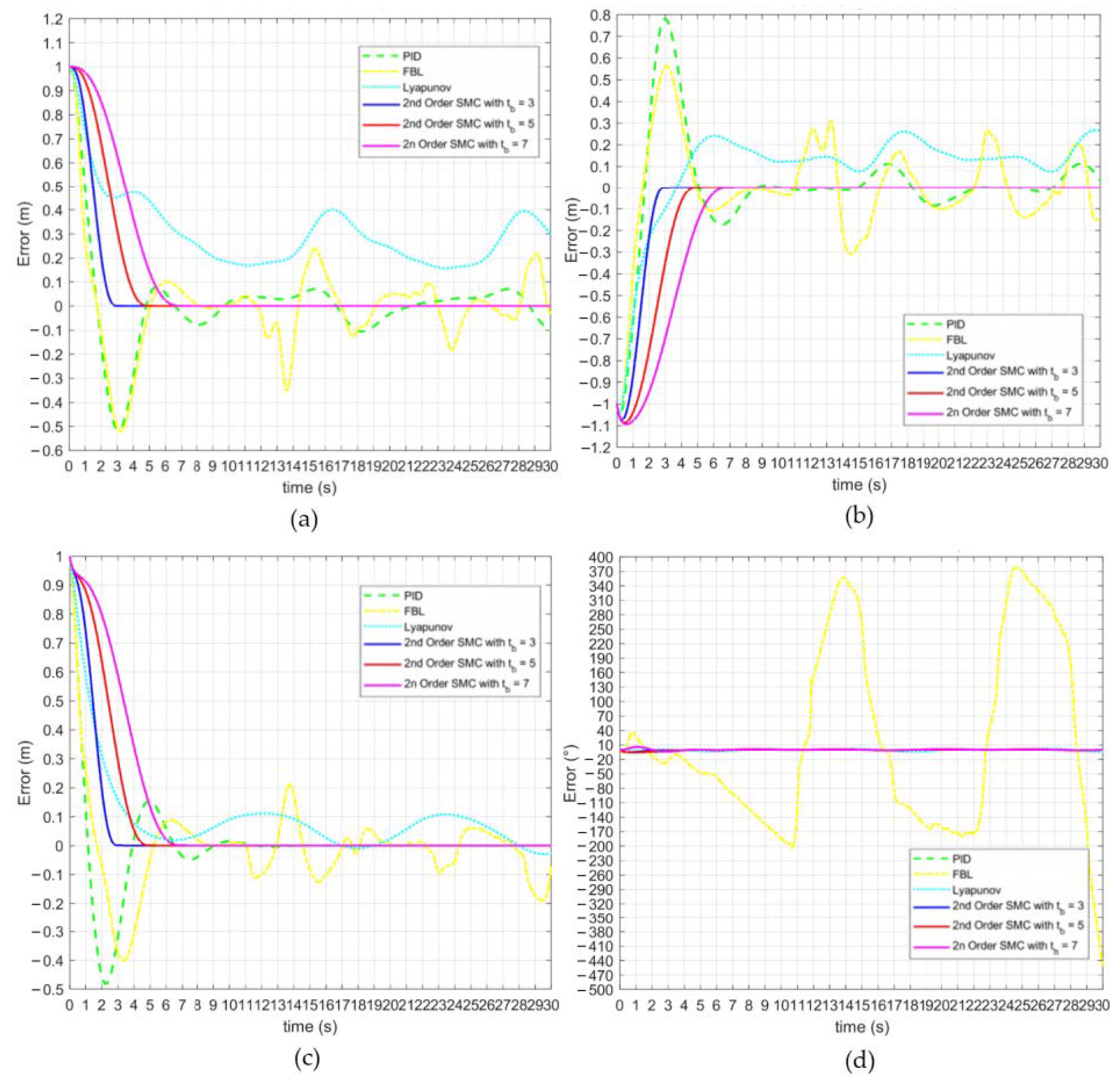
3.2. Considering Ocean Currents as Disturbances

The forces of the ocean currents can be considered constant and irrotational according to Fossen [30]; and can be implemented using relative velocity, which is the difference between the real velocity and the ocean current velocity

$${\nu }_{rel}=\nu - {\nu }_{oc},$$

(28)

where $\nu$ is the vehicle velocity and ${\nu }_{oc}$ is the ocean current velocity.

The generalized vector for an irrotational ocean current velocity is given by

$${\nu }_{oc}={\left[u_{oc},v_{oc},w_{oc},0,0,0\right]}^T,$$

(29)

where $u_{oc}$ is an ocean current velocity from the north, $v_{oc}$ is the ocean current velocity from the east, and $w_{oc}$ is the ocean current velocity from below.

Defining the angles ${\alpha }_{oc}$ as the angle of attack, and ${\beta }_{oc}$ as the slide slip angle, every element of the velocity vector can be calculated as

$$u_{oc}= {\nu }_{oc}cos{\alpha }_{oc}cos{\beta }_{oc},$$

$$v_{oc}={\nu }_{oc}sin{\beta }_{oc}, \mathrm{and}$$

$$w_{oc}= {\nu }_{oc}sin{\alpha }_{oc}cos{\beta }_{oc},$$

(30)

Since the velocity vector is expressed in the Earth-Fixed frame, Equation (4) can be modified resulting in

$$M{\dot{\nu }}_{rel}+C\left({\nu }_{rel}\right){\nu }_{rel}+D\left({\nu }_{rel}\right){\nu }_{rel}+g\left(\eta \right)= \tau ,$$

(31)

Zhang et al. [35] performed some experiments where high ocean currents affecting a UUV were measured. Taking them into account and for purposes of the simulations presented in this work, the following ocean currents will be included as constants

$$u_{oc}= 0.75 \frac{\mathrm{m}}{\mathrm{s}},$$

$$v_{oc}=0.25 \frac{\mathrm{m}}{\mathrm{s}}, \mathrm{and}$$

$$w_{oc}= 0.25 \frac{\mathrm{m}}{\mathrm{s}},$$

(32)

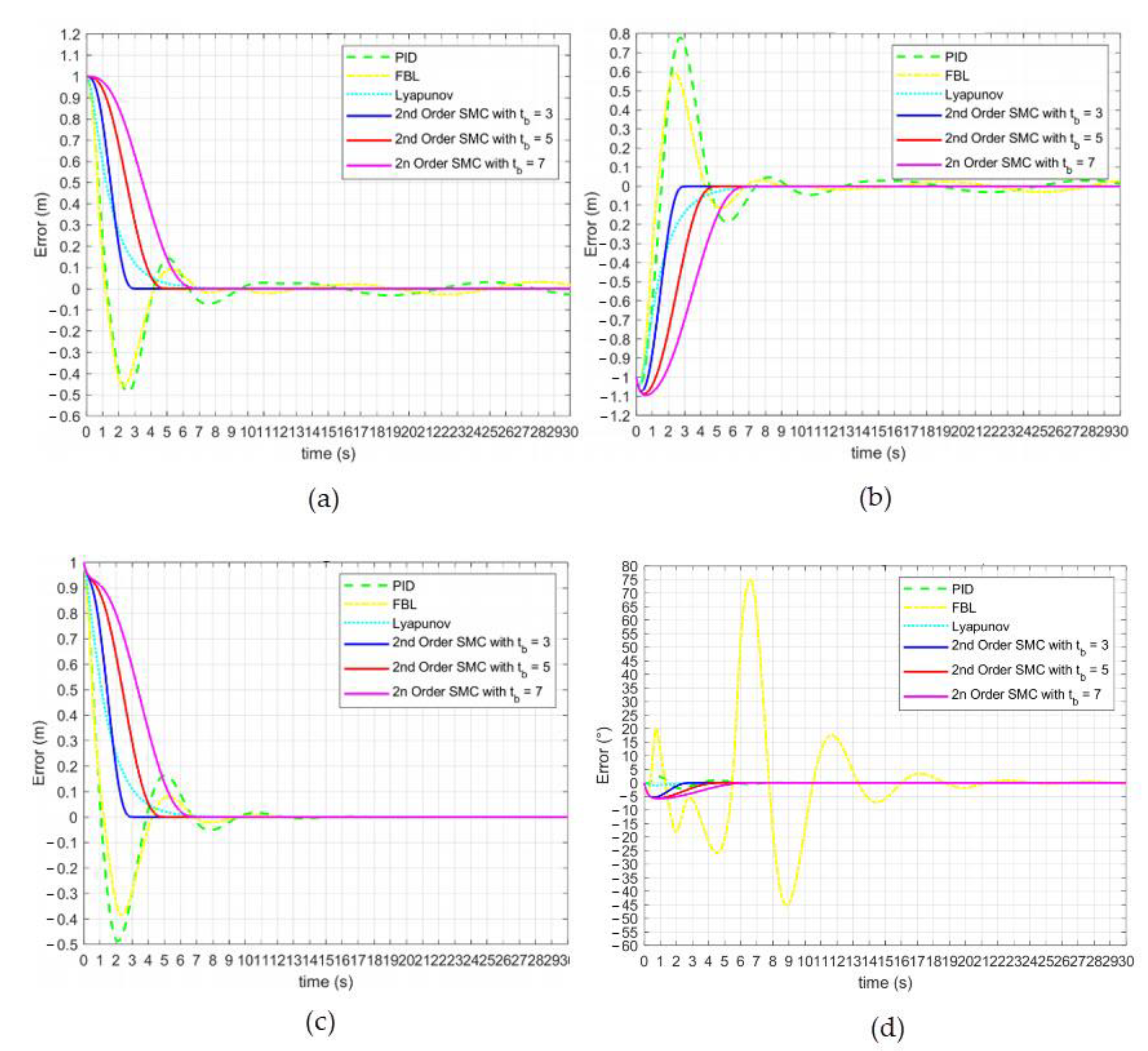
3.3. Comparing with Classic Controllers

Other classic control approaches such as PID, Feed-Back Linearization (FBL), and Lyapunov-based controllers [30], [36] will be simulated for the trajectory tracking of the BlueROV2 to compare the performance of the proposed model-free 2nd order SMC.

3.3.1. PID Controller

The control signal used for the PID controller is given by

$${\tau }_{\eta }=-K_p\tilde{\eta }-K_i{{\displaystyle \int }}^{}\tilde{\eta } dt-K_d \dot{\tilde{\eta }},$$

(33)

where $K_p$, $K_i$, and $K_d$ are the proportional, integral, and derivative gain matrices, respectively. An initial set of gain matrices was proposed and then several simulations were performed aiming to find the one that produces the best results for the trajectory tracking of all DOFs. As a result, the gain matrices for this controller are defined as

$$K_p= \mathrm{diag}\left[140,140,140,140,0,140\right],$$

$$K_i= \mathrm{diag}\left[120,120,120,120,0,120\right], \mathrm{and}$$

$$K_d= \mathrm{diag}\left[180,180,180,180,0,180\right],$$

(34)

3.3.2. Feed-Back Linearization Controller

The control signal used for the FBL controller is given by:

$$\tau =M{a}^b+C\left(\nu \right)\nu +D\left(\nu \right)\nu +g\left(\eta \right),$$

(35)

where $a^b$ is the commanded acceleration. Here, a PID controller will be used as an auxiliary controller to compute $a^b$ as

$$a^b={\dot{\nu }}_d-K_p\tilde{\nu }-K_i{{\displaystyle \int }}^{}\tilde{\nu } dt-K_d\dot{\tilde{\nu }},$$

(36)

where

$$\tilde{\nu }= \nu -{\nu }_d,$$

(37)

$K_p$, $K_i$, and $K_d$ will take the same values as in Equation (33).

3.3.3. Lyapunov-Based Controller

The control signal used for the Lyapunov-based controller is given by:

$$\tau =M{\dot{\nu }}_r+C{\nu }_r+D{\nu }_r+g\left(\eta \right)-K_{d}S,$$

(38)

where

$$S= \nu -{\nu }_{r },$$

(39)

$${\nu }_r=J^{-1}{\dot{\eta }}_r,$$

(40)

$${\dot{\nu }}_r= J^{-1}\left[{\ddot{\eta }}_r-\dot{J}{\nu }_r\right], \mathrm{and}$$

(41)

$${\dot{\eta }}_r={\dot{\eta }}_d- \alpha \tilde{\eta },$$

(42)

where $K$ and $\alpha$ are gain matrices which, after several iterations to find a suitable performance of the controller, will take the following values

$$K_d=diag\left[80,80,80,80,0,80\right], \mathrm{and}$$

$$\alpha =\left[0.80,0.80,0.80,0.80,0,0.80\right],$$

(43)

The values for the gain matrices used in the simulations of this work are summarized in

Table 3. Gain matrices for classic controllers and the proposed model-free 2nd order SMC with finite-time convergence.

Controller	${\mathit{K}}_{\mathit{p}}$	${\mathit{K}}_{\mathit{i}}$	${\mathit{K}}_{\mathit{d}}$	$\mathit{\alpha }$	$\mathit{\kappa }$
PID	140	120	180	-	-
Feed-back linearization	140	120	180	-	-
Lyapunov-based	-	-	80	0.80	-
Model-free 2nd order SMC with finite-time convergence	-	5	800	$\alpha \left(t\right)$	5

.

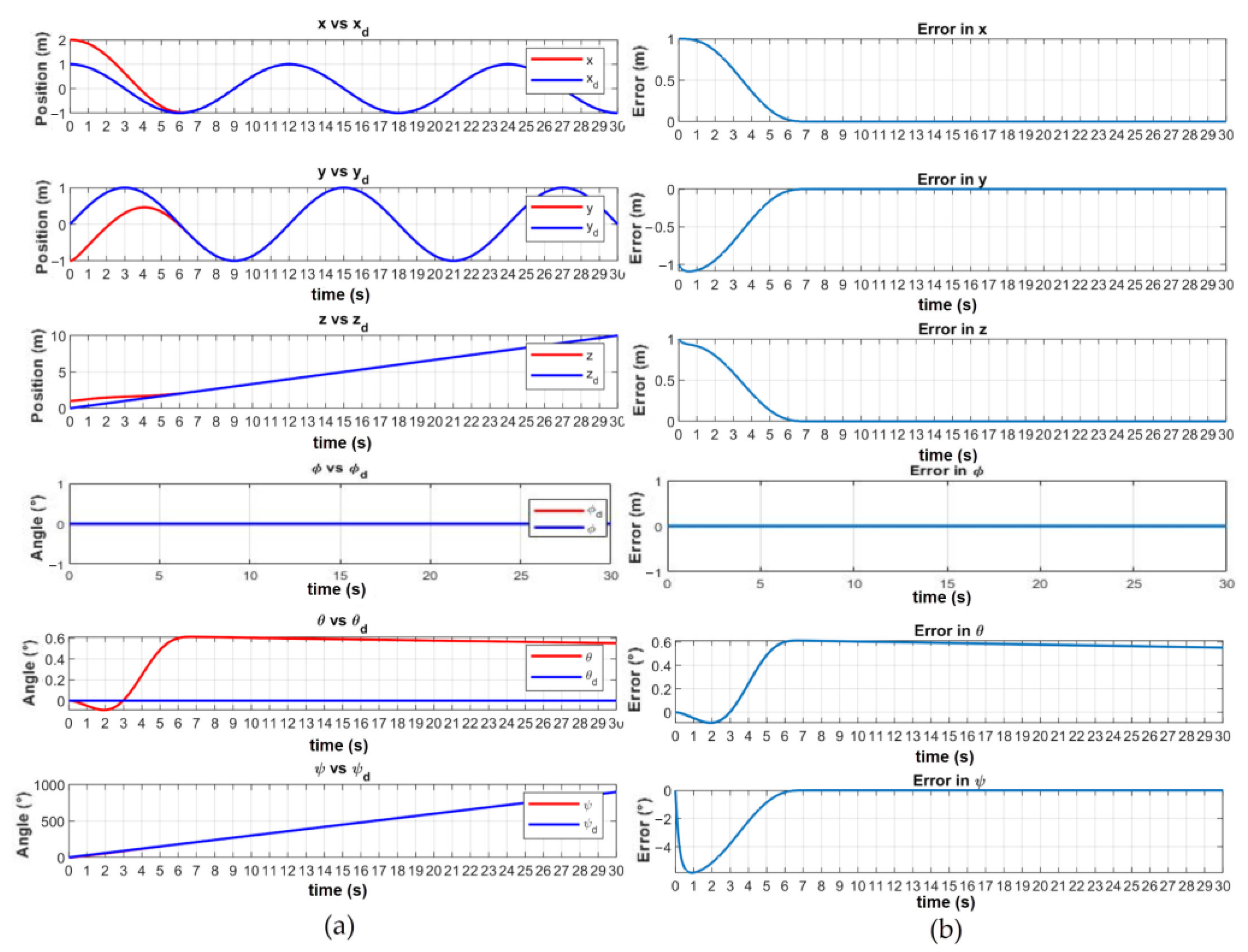
4. Results and Discussion

A simulation was performed so that a computational model of the BlueROV2 follow the spiral trajectory described before, the parameters and gains for the proposed model-free 2nd order SMC with finite-time convergence are shown in

Table 4. Controller parameters for simulation of a desired spiral trajectory.

Parameter	Value	Parameter	Value
$t_0$	0	$\delta$	0.001
$t_b$	5	$\kappa$	5
${\mathsf{\alpha }}_0$	1.01	$K_i$	$diag\left[0,5,5,5,5,5\right]$
${\mathsf{\alpha }}_c$	20	$K_d$	$diag\left[800,800,800,800,0,800\right]$

. The initial position for the vehicle was set to $x=2 \mathrm{meters}$, $y=-1 \mathrm{meter}$, and $z=2 \mathrm{meters}$ so it started slightly away from the desired trajectory. The effects of ocean currents were neglected for this simulation.

Results for trajectory tracking and errors of the proposed controller are presented in Figure 5. The controlled trajectory smoothly converged with the desired trajectory at the time-base proposed and without overshoots, after that, the vehicle followed the desired trajectory without deviations. The errors decreased over time to become zero at the designated $t_b$ except for the pitch, which, as established in Section 2.1, was not actuated and the resulting increase in its error—smaller than 0.5°—was caused by the vehicle’s dynamics while moving forward.

A three-dimensional trajectory of the BlueROV2 simulation along with the control trajectory can be seen in Figure 6.

The control coefficients for each of the BlueROV2 thrusters are shown in Figure 7. These control coefficients were in a range of $-1\le u\le 1$, where $\left|u\right|=1$ represents that the controller is demanding 100% of the thruster force. The maximum force was demanded at the start of the simulation and, after reaching the time-base, the control signals remained constant and no chattering was observed.

Since $t_b$ can be tuned arbitrarily for the user, further simulations were performed for the proposed controller under the same gains and parameters but for different time-bases. Simulation results for trajectory tracking and errors are shown in Figure 8 and Figure 9 for a time-base of 3 and 7 s, respectively. In both cases, the vehicle met the desired trajectory at the designated time-base $t_b$.

The controllers presented and described in Section 3.3 were simulated for comparing their error convergence to zero and the control coefficient computed for the BlueROV2 thrusters. As can be seen in Figure 10, the surge and sway error of the proposed controller converges to zero at the desired time. Meanwhile, the rest of the controllers converged at different times and, for the PID and FBL, there was not a stationary error but an oscillation in its value was observed through the simulated time. For the heave error, despite the oscillations resulting in the PID and the FBL, all the controllers converged to zero. Finally, for the yaw orientation, the FBL exhibited some troubles converging to zero during the first 20 s to finally converge to it exponentially. In general, the performance of the proposed model-free 2nd order SMC with finite-time convergence surpassed the rest of the controllers, even when FBL and Lyapunov-based were model-based.

To evaluate the performance of the proposed controller in terms of energy consumption from the thrusters, the Root Mean Square (RMS) value of the control coefficients computed for the thrusters was obtained and results are shown in

Table 5. Root Mean Square (RMS) values for thrusters control coefficients.

Controller	Thruster 1	Thruster 2	Thruster 3	Thruster 4	Thruster 5	Thruster 6	Mean
PID	0.2078	0.1946	0.2010	0.2105	0.1311	0.2041	0.1915
Feed-back linearization	0.1676	0.1876	0.1909	0.1693	0.2851	0.2760	0.2127
Lyapunov-based	0.1278	0.1500	0.1380	0.1192	0.0678	0.1358	0.1231
Model-free 2nd Order SMC with $t_b = 3 \mathrm{s}$	0.1449	0.1400	0.1333	0.1378	0.0801	0.1418	0.1296
Model-free 2nd Order SMC with $t_b = 5 \mathrm{s}$	0.1264	0.1175	0.0986	0.1059	0.0740	0.1324	0.1091
Model-free 2nd Order SMC with $t_b = 7 \mathrm{s}$	0.1132	0.1067	0.0880	0.0921	0.0726	0.1295	0.1004

. The mean column of the table represents the mean value of the coefficients considering all six thrusters. As it can be seen in the table, the average thruster force demanded by the proposed model-free 2nd order SMC was in the range of 0.1004 and 0.1296—1.0 being the maximum—this was up to 50% less than the forces demanded by a traditional PID or FBL controller even when it converged faster. The Lyapunov-based controller converged to the trajectory approximately at 7 s, and its mean value for control coefficient of the thrusters was 23% bigger than the 2nd Order SMC with ${\mathrm{t}}_b = 7 \mathrm{s}$.

To test the controller response to external disturbances, the effects of ocean currents were included as described in Section 3.2. Results for trajectory tracking and errors of a simulation with the proposed model-free 2nd order SMC with $t_b=5 \mathrm{s}$ are shown in Figure 11. Despite the high ocean currents introduced, the BlueROV2 still smoothly converged to the desired trajectory at the designated $t_b$, there were not overshoots at all, and the vehicle followed the designed trajectory with an error of zero after the time-base was reached.

A three-dimensional trajectory of the BlueROV2 simulation along with the control trajectory when subject to ocean currents can be seen in Figure 12.

Control signals for each of the BlueROV2 thrusters are shown in Figure 13. Contrary to the simulation results shown in Figure 7, the control signal did not remain constant after the time-base was reached. Thruster control signals changed over time to overcome the perturbations introduced by the ocean currents, which allowed the BlueROV2 to follow the desired trajectory as designed.

Ocean currents were also included in simulations for the rest of the controllers considered in the past section. Results for tracking errors are presented in Figure 14. None of the classic controllers tested were able to overcome the perturbations introduced, while the proposed model-free 2nd order SMC was able to compensate for them and keeping the finite-time convergence as designated by the user.

To evaluate the performance of the proposed controller in terms of energy consumption from the thrusters, the Root Mean Square (RMS) value of the control coefficients computed for the thrusters was obtained when the vehicle was subject to high ocean currents. Results are shown in

Table 6. RMS values for thrusters control coefficients when the vehicle is subject to high ocean currents.

Controller	Thruster 1	Thruster 2	Thruster 3	Thruster 4	Thruster 5	Thruster 6	Mean
PID	0.3254	0.3131	0.3534	0.3163	0.1135	0.1761	0.2663
Feed-back linearization	0.3978	0.4008	0.4056	0.3892	0.7889	0.7749	0.5262
Lyapunov-based	0.27321	0.2479	0.2607	0.2306	0.0578	0.0843	0.1924
Model-free 2nd Order SMC with $tb = 3 \mathrm{s}$	0.2790	0.2684	0.3093	0.2646	0.0578	0.0840	0.2105
Model-free 2nd Order SMC with $tb = 5 \mathrm{s}$	0.2909	0.2670	0.2801	0.2535	0.0500	0.0556	0.1995
Model-free 2nd Order SMC with $tb = 7 \mathrm{s}$	0.2897	0.2525	0.2625	0.2421	0.0479	0.0469	0.1903

.

The average thruster force demanded by the model-free 2nd order SMC with finite-time convergence was in a range of 0.1903 and 0.2105, which resulted in up to 30% less than the average force demanded by the PID controller and up to 64% less than the demanded by the FBL controller, even when they were not able to meet the trajectory and maintain the vehicle there.

5. Conclusions

Finite-time trajectory tracking of underactuated UUVs is a considerable challenge. Their nonlinear dynamics and the challenging conditions of the underwater environment make it more complex for the controller to achieve a stable and robust performance as they do in other systems and environments. In this work, for the first time, a model-free 2nd order SMC and a TBG were synthesized and implemented to achieve finite-time convergence of an underactuated nonlinear UUV to a desired trajectory. Such a controller has some advantages compared with other finite-time model-based 1st order SMC reported in literature since it neither requires the dynamic model structure nor the knowledge of any hydrodynamical parameter from the vehicle. In addition, this controller does not present the chattering effect common in other conventional SMC. The TBG was included in the controller by the parametrization of the $\alpha$ gain at the sliding surface, making it time-varying instead of constant. The hydrodynamical model of the BlueROV2 UUV was implemented in MATLAB/Simulink^®. There, numerical simulations were performed to validate the performance of the proposed controller. Results have shown that the controller was able to manage the BlueROV2 to smoothly converge to the desired trajectory at a specific time without overshoots, and then follow it with a tracking error of zero. Other classic controllers such as PID and FBL could not achieve a similar performance. Since the time-base can be tuned arbitrarily for the user, simulations were repeated with different time-bases and the results remained consistent and satisfactory. The performance of the solution proposed was also evaluated in terms of the energy consumption regarding the thruster forces demanded by the different controllers. It was shown that the proposed model-free 2nd order SMC demands up to 50% less power from the thrusters than other of the controllers simulated and it does not present the chattering effect common in some SMC controllers. Finally, the vehicle was subject to high ocean currents. Simulation results showed that the controller stills able to meet the desired trajectory at the designated time, smoothly and without overshoots, and then maintain the vehicle in the desired trajectory when other classic controllers could not. In future work, authors expect to verify the finite-time convergence of the model-free 2nd order SMC by performing experimentation under controlled conditions with the BlueROV2 vehicle whose hydrodynamical model was considered for the simulations presented in this work. Further research will also include the obstacle avoidance problem during the trajectory tracking.

References

1. Hartono, M.T.; Budiyanto, M.A.; Dhelika, R. Micro class underwater ROV (remotely operated vehicle) as a ship hull inspector: Development of an initial prototype. AIP Conf. Proc. 2020, 2227, 020025. [Google Scholar]
2. Buscher, E.; Mathews, D.L.; Bryce, C.; Bryce, K.; Joseph, D.; Ban, N.C. Applying a Low Cost, Mini Remotely Operated Vehicle (ROV) to Assess an Ecological Baseline of an Indigenous Seascape in Canada. Front. Mar. Sci. 2020, 7, 1–12. [Google Scholar] [CrossRef]
3. Sward, D.; Monk, J.; Barrett, N. A systematic review of remotely operated vehicle surveys for visually assessing fish assemblages. Front. Mar. Sci. 2019, 6, 1–19. [Google Scholar] [CrossRef] [Green Version]
4. Sandøy, S.S.; Hegde, J.; Schjølberg, I.; Utne, I.B. Polar Map: A Digital Representation of Closed Structures for Underwater Robotic Inspection. Aquac. Eng. 2020, 89, 102039. [Google Scholar] [CrossRef]
5. González-García, J.; Gómez-Espinosa, A.; Cuan-Urquizo, E.; García-Valdovinos, L.G.; Salgado-Jiménez, T.; Cabello, J.A.E. Autonomous Underwater Vehicles: Localization, Navigation, and Communication for Collaborative Missions. Appl. Sci. 2020, 10, 1256. [Google Scholar] [CrossRef] [Green Version]
6. Kumar, N.; Rani, M. An efficient hybrid approach for trajectory tracking control of autonomous underwater vehicles. Appl. Ocean Res. 2020, 95, 102053. [Google Scholar] [CrossRef]
7. Elmokadem, T.; Zribi, M.; Youcef-Toumi, K. Terminal sliding mode control for the trajectory tracking of underactuated Autonomous Underwater Vehicles. Ocean Eng. 2017, 129, 613–625. [Google Scholar] [CrossRef]
8. Rojas, J.; Baatar, G.; Cuellar, F.; Eichhorn, M.; Glotzbach, T. Modelling and Essential Control of an Oceanographic Monitoring Remotely Operated Underwater Vehicle. IFAC-PapersOnLine 2018, 51, 213–219. [Google Scholar] [CrossRef]
9. Dong, M.; Li, J.; Chou, W. Depth control of ROV in nuclear power plant based on fuzzy PID and dynamics compensation. Microsyst. Technol. 2020, 26, 811–821. [Google Scholar] [CrossRef]
10. Yang, M.; Sheng, Z.; Che, Y.; Hu, J.; Hu, K.; Du, Y. Design of Small Monitoring ROV for Aquaculture. In Proceedings of the OCEANS 2019—Marseille, Marseille, France, 17–20 June 2019; pp. 1–9. [Google Scholar]
11. Zhang, L.; Zhang, L.; Liu, S.; Zhou, J.; Papavassiliou, C. Low-level control technology of micro autonomous underwater vehicle based on intelligent computing. Cluster Comput. 2019, 22, 8569–8580. [Google Scholar] [CrossRef]
12. Hernández-Alvarado, R.; García-Valdovinos, L.G.; Salgado-Jiménez, T.; Gómez-Espinosa, A.; Fonseca-Navarro, F. Neural network-based self-tuning PID control for underwater vehicles. Sensors 2016, 16, 1429. [Google Scholar] [CrossRef] [Green Version]
13. Yan, Z.; Yang, Z.; Zhang, J.; Zhou, J.; Jiang, A.; Du, X. Trajectory tracking control of uuv based on backstepping sliding mode with fuzzy switching gain in diving plane. IEEE Access 2019, 7, 166788–166795. [Google Scholar] [CrossRef]
14. Yan, Z.; Wang, M.; Xu, J. Integrated guidance and control strategy for homing of unmanned underwater vehicles. J. Franklin Inst. 2019, 356, 3831–3848. [Google Scholar] [CrossRef]
15. Zhou, J.; Zhao, X.; Chen, T.; Yan, Z.; Yang, Z. Trajectory Tracking Control of an Underactuated AUV Based on Backstepping Sliding Mode with State Prediction. IEEE Access 2019, 7, 181983–181993. [Google Scholar] [CrossRef]
16. Huang, B.; Yang, Q. Double-loop sliding mode controller with a novel switching term for the trajectory tracking of work-class ROVs. Ocean Eng. 2019, 178, 80–94. [Google Scholar] [CrossRef]
17. Ramezani-al, M.R.; Tavanaei Sereshki, Z. A novel adaptive sliding mode controller design for tracking problem of an AUV in the horizontal plane. Int. J. Dyn. Control 2019, 7, 679–689. [Google Scholar] [CrossRef]
18. Lv, T.; Zhou, J.; Wang, Y.; Gong, W.; Zhang, M. Sliding mode based fault tolerant control for autonomous underwater vehicle. Ocean Eng. 2020, 216, 107855. [Google Scholar] [CrossRef]
19. García-Valdovinos, L.G.; Fonseca-Navarro, F.; Aizpuru-Zinkunegi, J.; Salgado-Jiménez, T.; Gómez-Espinosa, A.; Cruz-Ledesma, J.A. Neuro-Sliding Control for Underwater ROV’s Subject to Unknown Disturbances. Sensors 2019, 19, 2943. [Google Scholar] [CrossRef] [Green Version]
20. Qin, H.; Li, C.; Sun, Y.; Li, X.; Du, Y.; Deng, Z. Finite-time trajectory tracking control of unmanned surface vessel with error constraints and input saturations. J. Frankl. Inst. 2020, 357, 11472–11495. [Google Scholar] [CrossRef]
21. Yan, Z.; Yu, H.; Zhang, W.; Li, B.; Zhou, J. Globally finite-time stable tracking control of underactuated UUVs. Ocean Eng. 2015, 107, 132–146. [Google Scholar] [CrossRef]
22. Yu, H.; Guo, C.; Yan, Z. Globally finite-time stable three-dimensional trajectory-tracking control of underactuated UUVs. Ocean Eng. 2019, 189, 106329. [Google Scholar] [CrossRef]
23. Chu, Z.; Zhu, D.; Yang, S.X. Observer-based adaptive neural network trajectory tracking control for remotely operated vehicle. IEEE Trans. Neural Networks Learn. Syst. 2017, 28, 1633–1645. [Google Scholar] [CrossRef]
24. Qiao, L.; Zhang, W. Double-Loop Integral Terminal Sliding Mode Tracking Control for UUVs with Adaptive Dynamic Compensation of Uncertainties and Disturbances. IEEE J. Ocean. Eng. 2019, 44, 29–53. [Google Scholar] [CrossRef]
25. Guerrero, J.; Torres, J.; Creuze, V.; Chemori, A. Trajectory tracking for autonomous underwater vehicle: An adaptive approach. Ocean Eng. 2019, 172, 511–522. [Google Scholar] [CrossRef] [Green Version]
26. Parra-Vega, V.; Garcia-Valdovinos, L.; Dominguéz-Ramiréz, O.A. Sliding PID Control for Tracking in Finite Time for Robot Arms. In Proceedings of the 11th International Conference on Advanced Robotics, Coimbra, Portugal, 30 June–3 July 2003; pp. 1526–1531. [Google Scholar]
27. García-Valdovinos, L.G.; Parra-Vega, V.; Arteaga, M.A. Bilateral Cartesian sliding PID force/position control for tracking in finite time of master-slave systems. Proc. Am. Control Conf. 2006, 2006, 369–375. [Google Scholar] [CrossRef]
28. Garcia-Valdovinos, L.G.; Parra-Vega, V.; Mendez-Iglesias, J.A.; Arteaga, M.A. Cartesian sliding PID force/position control for transparent bilateral teleoperation. IECON Proc. Ind. Electron. Conf. 2005, 2005, 1979–1985. [Google Scholar] [CrossRef]
29. Perruquetti, W.; Barbot, J.-P. Sliding Mode Control in Engineering; Marcel Dekker Inc.: New York, NY, USA, 2002; ISBN 9780429222832. [Google Scholar]
30. Fossen, T.I. Handbook of Marine Craft Hydrodynamics and Motion Control; John Wiley & Sons, Ltd.: Chichester, UK, 2011; ISBN 9781119994138. [Google Scholar]
31. BlueRobotics. BlueROV2—Datasheet. 2019. Available online: https://bluerobotics.com/wp-content/uploads/2020/02/br_bluerov2_datasheet_rev6.pdf (accessed on 11 December 2020).
32. Lack, S.; Rentzow, E.; Jeinsch, T. Experimental Parameter Identification for an open-frame ROV: Comparison of towing tank tests and open water self-propelled tests. IFAC-PapersOnLine 2019, 52, 271–276. [Google Scholar] [CrossRef]
33. Wu, C. 6-DoF Modelling and Control of a Remotely Operated Vehicle. Master’s Thesis, Flinders University, Adelaide, Australia, 2018. [Google Scholar]
34. García-Valdovinos, L.G.; Salgado-Jiménez, T.; Bandala-Sánchez, M.; Nava-Balanzar, L.; Hernández-Alvarado, R.; Cruz-Ledesma, J.A. Modelling, Design and Robust Control of a Remotely Operated Underwater Vehicle. Int. J. Adv. Robot. Syst. 2014, 11, 1. [Google Scholar] [CrossRef] [Green Version]
35. Zhang, S.; Yu, J.; Zhang, A.; Zhang, F. Spiraling motion of underwater gliders: Modeling, analysis, and experimental results. Ocean Eng. 2013, 60, 1–13. [Google Scholar] [CrossRef]
36. Do, K.D.; Pan, J. Control of Ships and Underwater Vehicles; Springer Science & Business Media: London, UK, 2009; ISBN 978-1-84882-729-5. [Google Scholar]
Figure 1. Reference frames needed to describe the BlueROV2.
Applsci 11 01836 g001
Figure 2. BlueROV2 thruster configuration. (a) Right view. (b) Top view.
Applsci 11 01836 g002
Figure 3. Model-free high-order Sliding Mode Control (SMC) with Time Base Generator (TBG) scheme.
Applsci 11 01836 g003
Figure 4. Parameterized desired spiral trajectory of the Unmanned Underwater Vehicle (UUV) BlueROV2.
Applsci 11 01836 g004
Figure 5. Results with t b   =   5   s . (a) Trajectory tracking. (b) Position tracking errors.
Applsci 11 01836 g005
Figure 6. Simulated three-dimensional trajectory of the BlueROV2 with t b   =   5   s .
Applsci 11 01836 g006
Figure 7. Control signal for each thruster. Simulation with t b   =   5   s .
Applsci 11 01836 g007
Figure 8. Results with t b =   3   s . (a) Trajectory tracking. (b) Position tracking errors.
Applsci 11 01836 g008
Figure 9. Results with t b   =   7   s . (a) Trajectory tracking. (b) Position tracking errors.
Applsci 11 01836 g009
Figure 10. Error convergence for different controllers. (a) Surge error. (b) Sway error. (c) Heave error. (d) Yaw error.
Applsci 11 01836 g010
Figure 11. Results for the finite-time convergence controller subject to ocean currents and t b = 5   s . (a) Trajectory tracking. (b) Position tracking errors.
Applsci 11 01836 g011
Figure 12. Simulated three-dimensional trajectory of the BlueROV2 when subject to ocean currents and t b = 5   s .
Applsci 11 01836 g012
Figure 13. Control signal for each thruster when subject to ocean currents and t b = 5   s .
Applsci 11 01836 g013
Figure 14. Error convergence for different controllers when subject to high ocean currents. (a) Surge error. (b) Sway error. (c) Heave error. (d) Yaw error.
Applsci 11 01836 g014