1. Introduction
Structural health monitoring (SHM) has been identified as a key technology for the operation and maintenance of future civil, naval, and aerospace structures. An ideal SHM system uses sensors embedded on the structure to provide a real-time assessment of structural integrity. This leads to a reduction in maintenance cost, time, and an overall improvement in structural safety. A variety of SHM methodologies are currently available in the open literature. The primary approach for damage detection is a comparison between the damaged and healthy state of the structure, using certain damage sensitive mechanical features. Some of the most popular SHM methods are based on modal parameters of the structure, where changes in the natural frequencies or mode shapes are used as damage indicators [
1]. Similarly, techniques that investigate slope or curvature discontinuities (caused by damage) in the mode shapes have been applied to beam [
2,
3] and plate [
4,
5,
6] structures. Data-normalization procedures based on machine learning have also been developed to improve SHM performance under the influence of different operational and environmental conditions [
1]. Aside from modal parameters, methods that analyze the strain or displacement field are also used. Here, damage can be detected using inverse modeling approaches [
7] or directly by examining the strain or displacement field for any violations of the governing differential equations of the structure [
8,
9]. The use of fiber optic strain sensors has become increasingly common [
10], due to their small size, resistance to electromagnetic interference, reliability, and resistance to weathering and corrosion, making them ideal candidates for long-term health monitoring applications. These advantages have seen them being widely used for SHM of civil structures such as bridges and tunnels [
11,
12], structures subjected to seismic loads [
13], and for monitoring offshore wind turbine structures [
14]. The possibility of embedding the fiber within a structure has seen its growing use in aerospace applications. Some of these applications include monitoring of future inflatable space habitats [
15] and composite structures, like an aircraft wing box [
16,
17].
In this context, the use of shape sensing methods for developing strain or displacement-based SHM systems is hugely appealing. Shape sensing refers to the inverse problem of reconstructing the displacement field of a structure using discrete surface strains. The reconstructed strain or displacement field can be analyzed to reveal the presence of damage on the structure. Current shape-sensing methods vary depending on their theoretical approaches to displacement reconstruction. Methods based on integrating experimental strains [
18] and using basis functions to approximate the displacement field [
19] have been used widely, while the use of neural networks (NN) has also been explored [
20].
Another approach for shape sensing is based on a variational principle, such as the inverse Finite Element Method (iFEM). The iFEM is based on discretizing the structural domain into a set of finite elements. The displacement field is obtained by minimizing an error functional defined as the least-square error between the analytic and experimental strain measures [
21,
22]. The iFEM has been developed for 1D beams and frames [
23], 2D plates and shells [
24,
25], and multi-layered composite and sandwich plates [
26,
27]. The iFEM can analyze both the static and dynamic response of a structure [
23,
28], in the linear and non-linear displacement regimes [
29], without any prior knowledge of the structure’s material properties or loading conditions. The use of iFEM for SHM has been demonstrated on simple beams using fiber optic strain measurements [
30] and on thin plates using strain measurements from a grid of strain rosettes [
31,
32].
The majority of aforementioned iFEM applications used tri-axial strain rosette measurements. In the few cases, where uniaxial strain data were considered, the primary focus was on reconstructing simple membrane or bending deformations of the structure [
27,
30]. Due to the high measurement density and operational convenience of a fiber optic system, there is enormous potential in using fiber optic strain measurements for the iFEM reconstruction. A possible application is for the SHM of plates or shells, where potential damage can cause local perturbations in the strain field. An accurate reconstruction of these 2D strain perturbations can provide useful information to identify the size, position, and orientation of the damage. However, in comparison with a strain rosette, strain measurements from a fiber optic sensor are uniaxial, i.e., only the component of strain along the local fiber direction is measured. iFEM reconstruction using only uniaxial strain data could lead to errors due to insufficient information regarding the strain field of a structure.
This work addresses the problem of damage detection in a thin cracked plate under the action of in-plane loading. Strain reconstruction is performed using the iFEM methodology in the presence of the discrete uniaxial strain data resulting from several fiber-optic strain sensor patterns. The approach also examines the use of a one-dimensional smoothing algorithm for generating additional input strain data along the paths of the fiber optic sensors. The paper is organized as follows. In
Section 2, an iFEM formulation for plate/shell structures is briefly described. In
Section 3, the use of iFEM for strain field reconstruction using uniaxial strain data is demonstrated using an example problem of a biaxially loaded thin plate under various internal damage scenarios. The effect of position and orientation of uniaxial strain data are investigated, and the damage detection performance of the reconstructed strain field is also discussed. Finally,
Section 4 presents the major conclusions and directions for future work.
2. The Inverse Finite Element Method
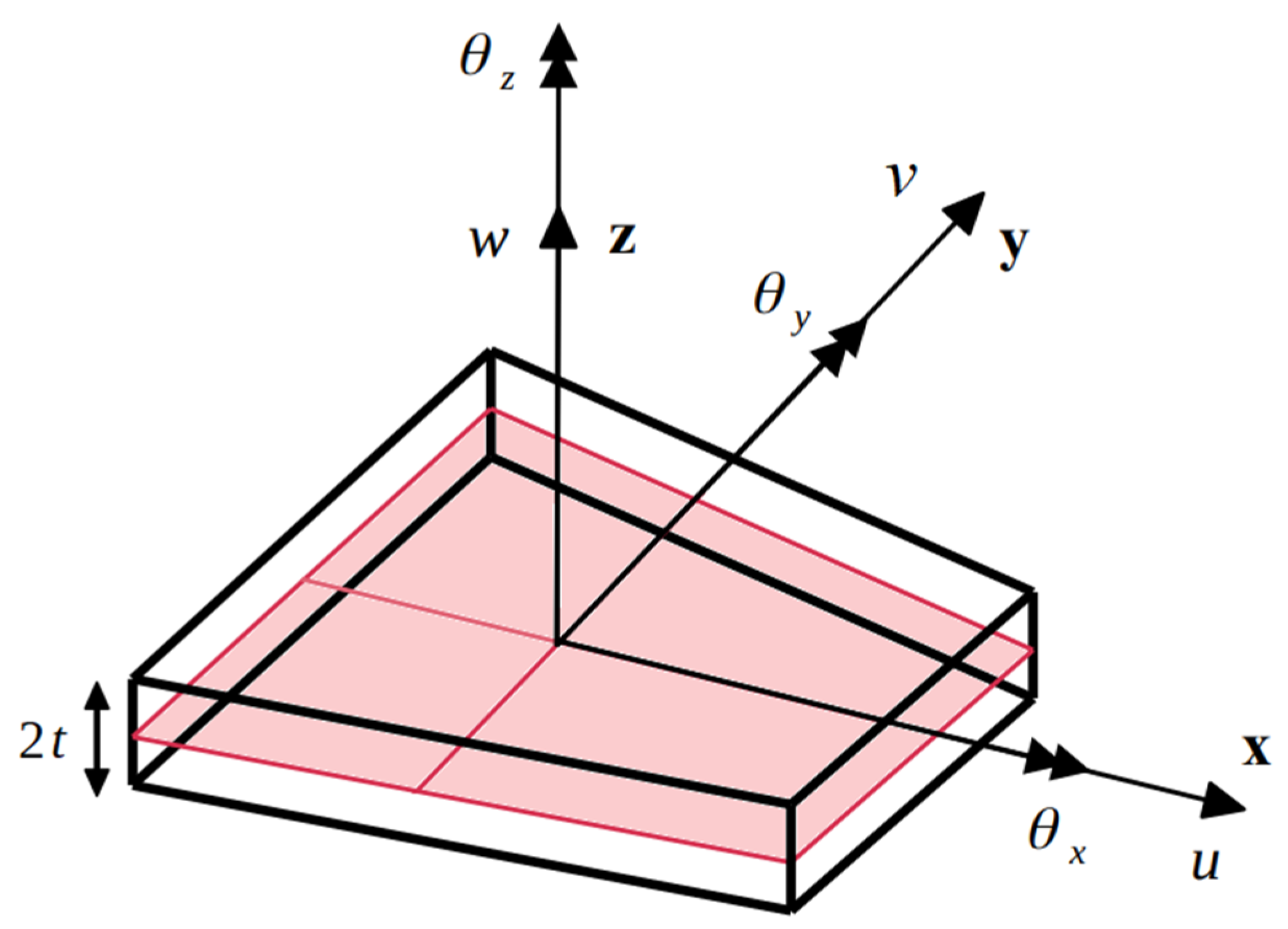
The iFEM formulation for plate/shell structures is based on the kinematic assumptions of Mindlin plate theory [
21,
22]. For a plate of thickness, 2
t, lying in a cartesian coordinate system, the components of the displacement vector are expressed as
where
and
are the kinematic variables associated with the mid-plane of the plate and are used to describe the displacement vector at any point of the structure. Variables
and
are average displacements along the
and
axis, respectively;
are the bending rotations about the
and
axis, respectively (see
Figure 1).
The linear strain displacement relations are used to obtain the strain field from the displacement assumptions of Equation (1)
The strain field of Equation (2) is represented by six strain measures; three membrane strain measures,
, representing the in-plane stretching of the mid-plane, and three bending strain measures,
, representing the bending and twisting curvatures. Additionally, Mindlin theory gives rise to two transverse shear strain measures,
. The eight strain measures are given as
Throughout this study, a four-node plate/shell element, iQS4 [
25], is used. The element is formulated using a set of anisoparametric C
0-continuous shape functions that enabled improved kinematic interdependency between the bending and shear deformations. Using the element shape functions, the strain measures can be expressed in terms of the element nodal degrees-of-freedom (DOF)
where
and
are matrices of shape function derivatives corresponding to the membrane, bending, and transverse shear strains, respectively. The vector,
, representing the element DOF of each element,
e, can be expressed as
where
denotes the vector of nodal DOF for each node
i, and
denotes the total number of nodes of the element. The membrane and bending strain measures,
and
, corresponding to experimental surface strain measurements at any location (
), are evaluated as
where
and
, are the in-plane normal and shear strains measured on the top and bottom surface of the structure, respectively, and
refers to the total number of strain-sensor locations corresponding to the mid-plane coordinates (
).
The iFEM variational formulation is based on a weighted-least squares error functional that minimizes the least-square errors between the analytic and experimental strain measures. The structural domain is discretized using the customary finite element framework, and the individual inverse finite elements are formulated on the basis of the error functional, given as
where
and
are vectors of weighting coefficients associated with the squared norms. The weighting coefficients are used to enforce a stronger or weaker correlation between the experimental strain measures and those described analytically. In elements where experimental strain measures are known, the coefficient vectors were assigned a value of unity (
,
), and the squared norms are expressed as
where
is the element area. In specific situations of a pure membrane or bending behavior, Equations (6) and (7) can be simplified further. When the plate is only under in-plane loads, the in-plane normal and shear strains on the top and bottom surfaces of the plate are equal. Strain measurements on only one surface of the plate are required to calculate
using Equation (6). In this case, the bending curvatures
in Equation (7) vanish identically. Similarly, when the plate is under pure bending, the strains on the top and bottom surfaces have the same magnitude with opposing signs (tension and compression). Measurements on only one surface of the plate are required to calculate
, whereas the membrane strain measures
vanish identically. In elements, where the experimental strain measures are unknown (due to the absence of experimental data), the coefficient vectors are assigned a relatively small value (
,
), and the corresponding squared norms reduce to
In cases where only specific components of membrane, bending, or transverse shear strains are experimentally measured at a point, two different strategies can be used for calculating the error functional of Equation (8). The first approach uses a suitable definition of the corresponding weighting coefficient vector. When using uniaxial strain sensors, where only specific components of the in-plane strains are measured at a point, the weighting coefficient vector for the membrane squared norms,
, is defined accordingly. For example, if the in-plane strain along the
x-axis (
) is the only strain component measured at a point. Then the corresponding weighting coefficient vector could be set as,
. The use of a small value for the weighting coefficient reduces the contribution of those unknown strain components to the element error functional. The second approach employs a smoothing technique. The smoothing technique uses the existing
strain measurements to obtain a smoothed value of
at points with no strain data. Using this approach, all unknown components of the membrane, bending or transverse shear strain measures, not experimentally measured at a point, can be obtained by smoothing strain data from other measurement locations of the plate. The latter approach is used in the current work; a detailed explanation of the steps involved is discussed in
Section 3.
The transverse shear strain measure,
, cannot be obtained directly using experimental strain measurements. Hence, the transverse shear squared norm (defined in Equation (10)) is associated with a small value of the corresponding weighting coefficient vector (
) for all elements. The error functional,
, is solved by minimizing with respect to the nodal DOF, yielding a set of linear algebraic equations
where the matrix,
, and vector,
, are functions of the strain sensor positions and measured surface strain data, respectively. Both
and
can be expanded and given as
Since the above terms involve area integrals, a suitable numerical integration scheme was used. The global matrices and vectors can be assembled by summing up the contributions from all the inverse elements,
,
where matrix,
, represents the element coordinate transformation matrix. The finite element assembly results in the global system of algebraic equations, given as
The solution of Equation (14) involves the application of the requisite displacement boundary conditions to restrain the structure against a rigid-body motion. Subsequently, provided is non-singular, the DOF vector, , can be uniquely determined.
3. Numerical Studies
The application of the iFEM method for strain field reconstruction using uniaxial strain data is presented using an example problem of a biaxially loaded square plate. The reconstructed strain field is further assessed to detect the presence of damage on the plate. The plate had a length
L = 3.8 m, thickness 2
t = 3.8 mm, and is made of an Aluminium alloy (Young’s modulus, E = 73 GPa, and Poisson’s Ratio, ν = 0.3). The plate is subjected to a uniform biaxial load of magnitude 10
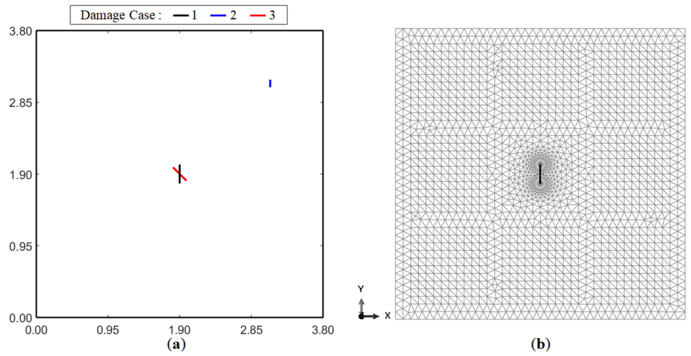
5 N/m. The damage on the plate is modeled as a crack, and three different damage scenarios of the plate (varying size, position, and orientation of the crack) are investigated (see
Figure 2a),
Damage Case-1: a 25 cm long crack is embedded at the center of the plate (crack position coordinates, ), with the crack front parallel to the vertical axis.
Damage Case-2: a 10 cm long crack is embedded near the corner of the plate (), with the crack front parallel to the vertical axis.
Damage Case-3: a 25 cm long crack is embedded at the center of the plate (), with the crack front oriented at 450 with the vertical axis.
Because of the pure membrane loading involved in this example problem, only the first term in Equation (8) is relevant for this iFEM application [
33]. This is because the membrane response is totally decoupled from the bending and transverse-shear deformations.
A high-fidelity FE model of the plate is developed in ABAQUS using the S3R element, a 3-node constant-strain shell element with reduced integration. A mesh convergence study is performed to ensure the convergence of the FE results. The FE model provided the simulated experimental strain measurements required for the iFEM analysis. The embedded crack is modeled in ABAQUS using the seam feature [
34], which created a set of overlapping duplicate nodes along the crack front. The FE model for Damage Case-1 used a total of 3368 elements, with a dense mesh near the crack tip (see
Figure 2b). The uniform biaxial loading condition is implemented in the FE model by prescribing a uniform distributed load on the top and right edge of the plate and imposing symmetric displacement boundary conditions on the left and bottom edge of the plate. The iFEM analysis is carried out using the 4-node iQS4 element [
25]. The iFEM mesh used has 16 elements along the plate length, leading to a total of 256 inverse elements (mesh is shown in
Figure 3). The absence of suitable displacement boundary conditions in the iFEM model can lead to a singular system matrix,
K (see Equation (14)), resulting in no available iFEM solution. Hence, the present iFEM model used symmetric displacement boundary conditions on the left (
), and bottom (
) edge of the plate (similar to the FE model).
The results of the iFEM reconstruction are presented as contour plots of the maximum principal strain
A damage index,
, which provides a normalized value of
within the range [0,1] is also proposed
where
and
define the minimum and maximum values of
for a reconstructed strain field. The damage index is used in setting thresholds for damage localization.
3.1. Benchmark iFEM Results
Before investigating the effects of uniaxial strain data, iFEM reconstruction using strain data measured by a dense grid of strain rosettes is used to establish a set of benchmark iFEM results. These results corresponded to a high accuracy iFEM reconstruction and are used as reference results for forthcoming comparisons. As the plate is under biaxial loading, in-plane strains are uniform across the plate thickness. Hence, only strain measurements made either on the top or bottom surface of the plate are required for calculating the experimental strain measures. In the present work, strain measurements made on the top surface of the plate are used. Membrane strain measures,
could be calculated using Equation (6)), while the bending strain measures,
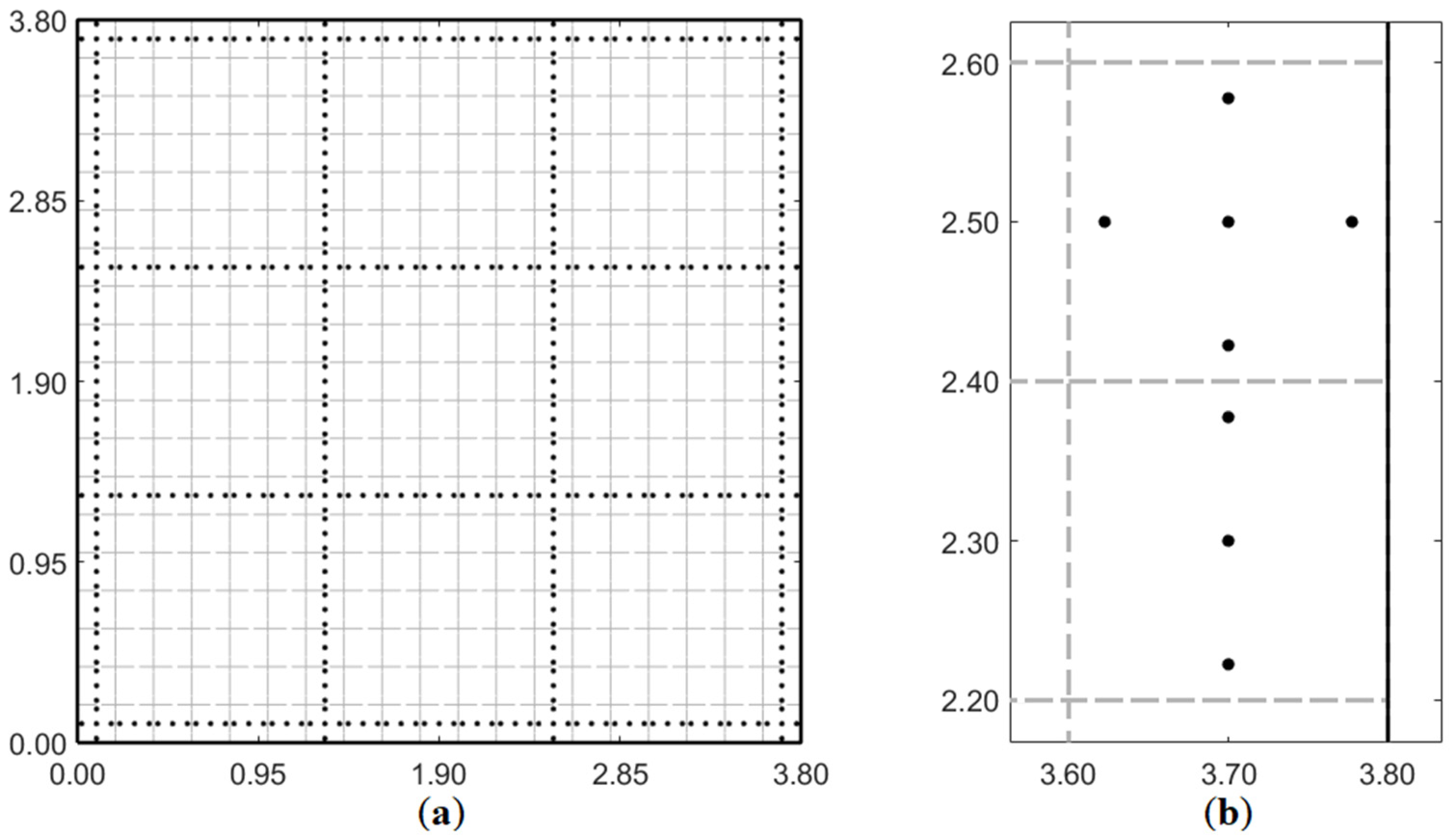
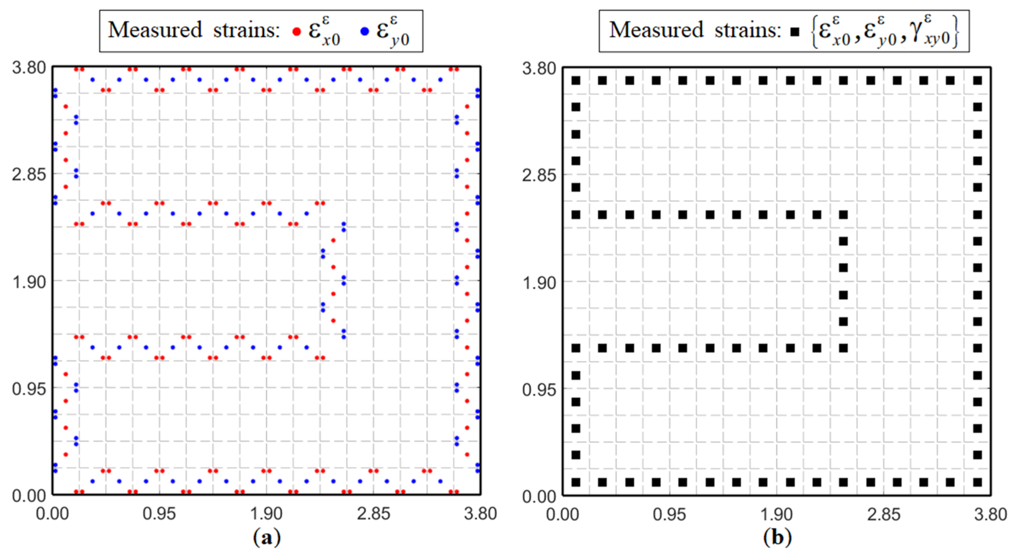
are equal to zero (Equation (7)). The sensor configuration used for the benchmark results is shown in
Figure 3a, where each point designates a strain rosette, and a total of 440 strain rosettes are used. Such a sensor grid divided the plate into nine square cells, where strain measurements are performed only along the cell boundaries. At each sensor position, the
and
components of strain are measured.
Figure 3b shows a magnified view of the sensor positions within some boundary elements. Depending on element position, strain measurements are available in at least three and at most five points within each element. For this analysis, the integrals of Equation (12) are integrated numerically using the 3 × 3 Gauss scheme.
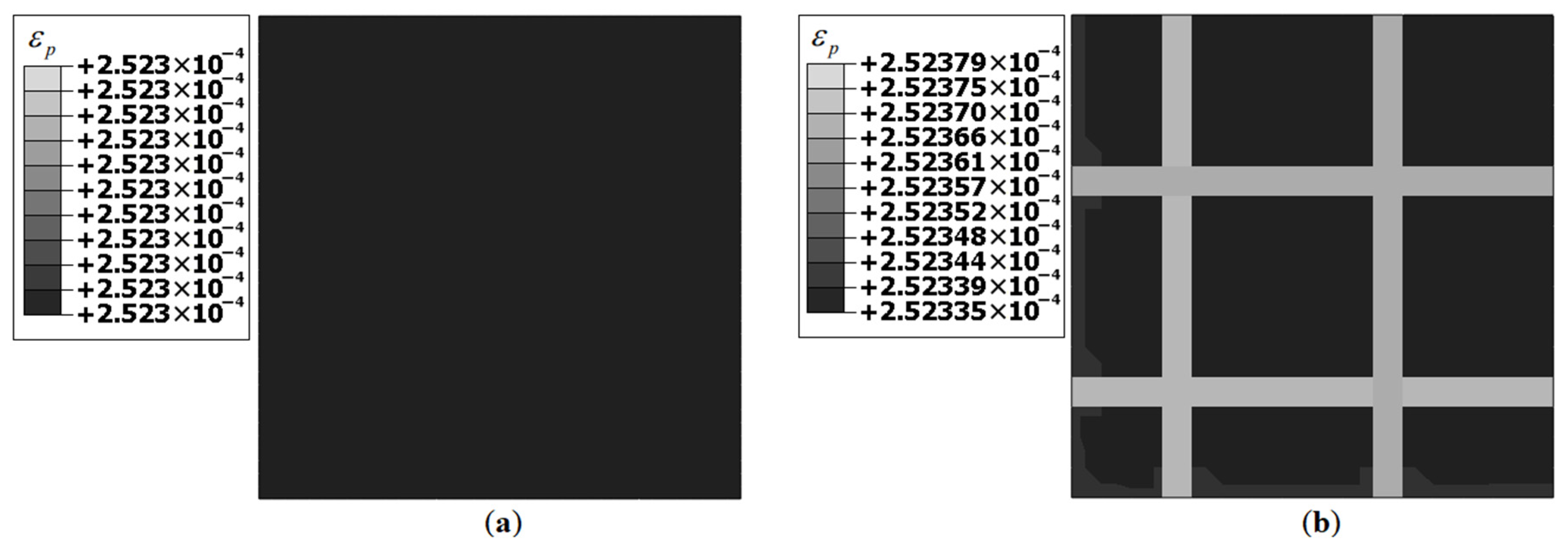
Initially, the benchmark iFEM model is used to reconstruct the strain field of an undamaged plate under biaxial loading. The FE and benchmark iFEM results for an undamaged plate are shown in
Figure 4. As the plate is under uniform biaxial loading, the in-plane normal strains are uniform, and the shear strain is negligible. Hence,
is a constant over the plate, as evident from the FE results (see
Figure 4a). The contour plot of iFEM results also showed a constant value of
, with minor variations of the order of 10
−8 (which are negligible). Accurate reconstruction of the undamaged far-field strains is essential for the damage detection strategy presented, as it acted as the baseline strain field of the structure. The present results clearly demonstrated the accuracy of the benchmark iFEM model in reconstructing the undamaged strain field. Next, the reconstruction accuracy of a damaged strain field is investigated.
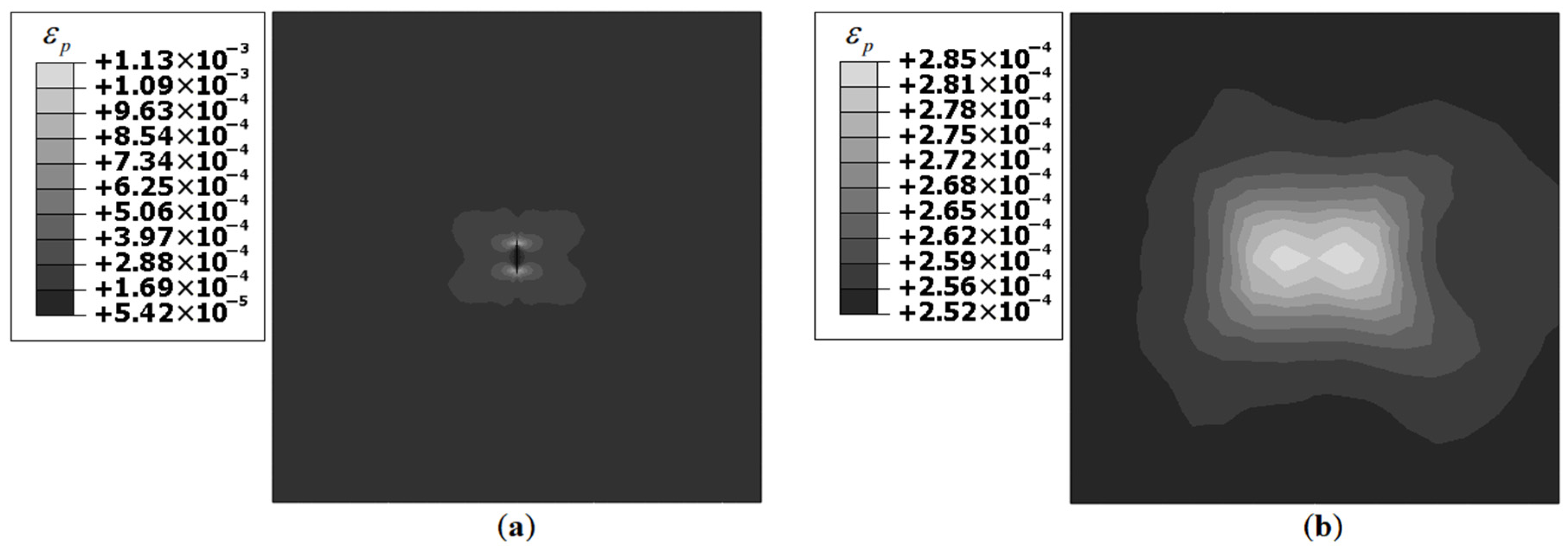
The FE and benchmark iFEM results for Damage Case-1 are shown in
Figure 5. Both plots showed a strain concentration in the vicinity of the crack, with the iFEM results having a more diffuse distribution and a lower magnitude of
. This is due to the absence of strain measurements close to the crack tip. The iFEM reconstruction utilized strains measured by the grid of sensors around the crack (see
Figure 3), and the sensors measured a lower strain magnitude than at the crack tip. This resulted in a lower magnitude and a more diffuse strain distribution in the iFEM results. Nevertheless, for damage detection, the iFEM results of
Figure 5b are promising as they successfully reconstructed a strain concentration at the damage site.
The FE and benchmark iFEM results for Damage Case-2 are shown in
Figure 6. In this case, the magnitude of
is smaller due to the smaller damage size. The FE results are highly localized, and the iFEM results showed a more diffuse
distribution at the damage site. The minimum value of
(corresponding to far-field strains) is similar in both plots of
Figure 6. This further corroborated the conclusions derived from
Figure 4, that the iFEM is accurate in reconstructing the undamaged far-field strains of the plate.
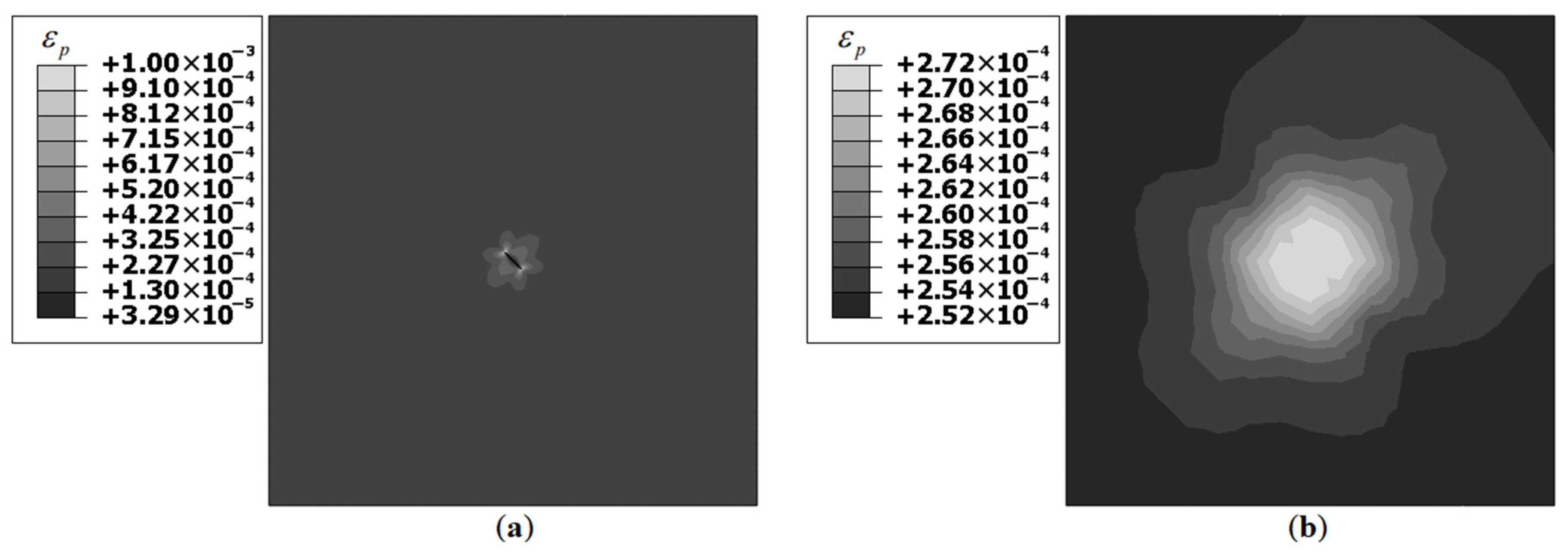
The results for Damage Case-3 are shown in
Figure 7. The inferences here are similar to those of Damage Case-1, except for a key feature, i.e., the strain field orientation. Both FE and iFEM results showed a greater
distribution perpendicular to the crack front, i.e., oriented at 45
0 with respect to the horizontal axis. This indicated that information regarding damage orientation could also be obtained by analyzing the reconstructed strain field.
The following conclusions could be drawn from the benchmark iFEM results. The iFEM procedure successfully reconstructed the far-field strains since the strain sensors are located far from the vicinity of the crack. Nevertheless, the presence and location of damage could be inferred from the iFEM results by contrasting the local strain peaks with the far-field strains (that acted as a healthy baseline state of the structure). It is noted that although a highly accurate reconstruction of the damaged strain field across the entire plate domain is preferred, it is not a prerequisite for the presented damage detection methodology. The current study aimed to maximize reconstruction accuracy and minimize the number of sensors used so that meaningful conclusions could be drawn from the reconstructed strain field for the purpose of damage detection. For the damage cases investigated, damage detection is successful regardless of the damage size and orientation. Although these benchmark results are promising, using such a large number of strain rosettes (440) may be generally impractical. This limitation could be overcome by using fiber optic strain sensors as discussed in the next section.
3.2. iFEM Studies Involving Uniaxial Strain Data
Fiber optic sensors are ideal candidates for strain field reconstruction using iFEM as they can provide a dense set of strain measurements over the fiber length. A typical strain rosette measurement system comprises sensors attached via a cable network to a Data Acquisition (DAQ) system. The measurements are processed into viable information and are subsequently stored and analyzed for decision making. In comparison, the cable network of a fiber optic system is composed entirely of the fiber with strain measurements all along the fiber length. The instrumentation systems used for fiber optic sensors depend on the specific sensing technology used [
10]. A distributed fiber optic system uses an interrogator to transmit optical pulses into the fiber and capture the backscattered light. The backscattered light is subsequently analyzed to obtain strain measurements along the fiber. In contrast to strain rosettes, fiber optic strain measurements are uniaxial, i.e., along the local fiber direction. Uniaxial strain measurements cannot provide all the components of in-plane strain (
) at a point, leading to inaccuracies in the iFEM reconstruction. The number and position of strain sensors used also affects the iFEM solution. Sensor configurations with an insufficient number of boundary elements with available strain data can lead to a singular system matrix and a breakdown of the iFEM solution. Similar is the case for configurations with discontinuous sensor patterns. Any proposed sensor configuration should avoid these conditions to ensure accurate iFEM results. In what follows, we describe efforts to reconstruct the strain field in a damaged plate using spatially distributed uniaxial fiber-optic strain sensors. The results are compared with the benchmark iFEM results of
Section 3.1.
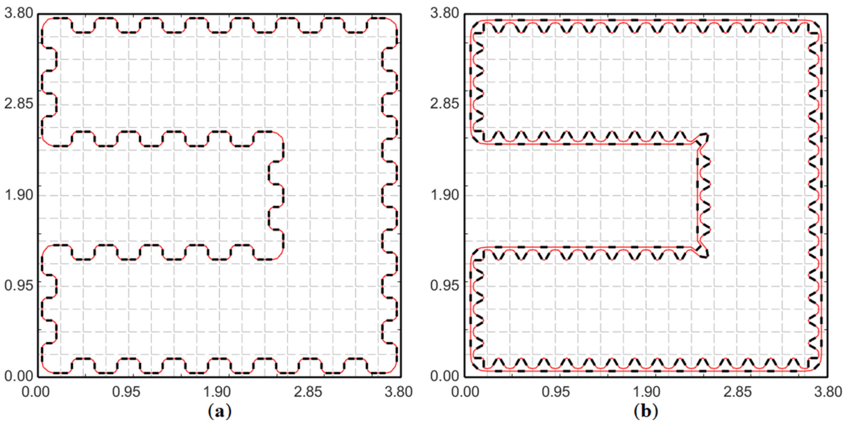
As the location and orientation of the strain measurements depend on the fiber arrangement, different fiber patterns are investigated. The plate is assumed to be instrumented with one or two continuous fibers to recreate the sensor pattern of the benchmark model (
Figure 3). The fiber arrangement should also maximize the quality and quantity of strain measurements, minimize fiber length, and avoid any self-intersections. Based on these requirements, two fiber arrangements are proposed (see
Figure 8),
Configuration-1: a continuous non-intersecting fiber arranged as a wave on the plate. The fiber arrangement within an element is referred to as ‘Unitcell-1’ (
Figure 9a), having the same pattern repeated across multiple elements. Strain measurements corresponding to Unitcell-1 are along the directions:
, which is a mixture of
and
strain data at different 3 × 3 Gauss integration points within an element. At most, three strain measurements are made per element.
Configuration-2: two continuous non-intersecting fibers are used to create a strain rosette within each element [
35]. The fiber arrangement within an element is referred to as ‘Unitcell-2’ (
Figure 9b), and the pattern is repeated across multiple elements. Strain measurements corresponding to Unitcell-2 are along directions:
. These three measurements formed a strain rosette and are used to calculate the
and
components of strain at the centroid of each element (
Figure 9b).
Strain measurements corresponding to Unicells-1 and 2 suffered from certain limitations. The fiber arrangements of
Figure 8 are unable to replicate the benchmark pattern of
Figure 3, resulting in certain boundary elements of the plate without any strain data (see
Figure 10), potentially leading to a singular system matrix,
K. This issue could be readily resolved by a pre-processing procedure that would enable these elements to be populated with strain data. For this purpose, a one-dimensional (1D) version of the Smoothing Element Analysis (SEA) [
36] is used herein.
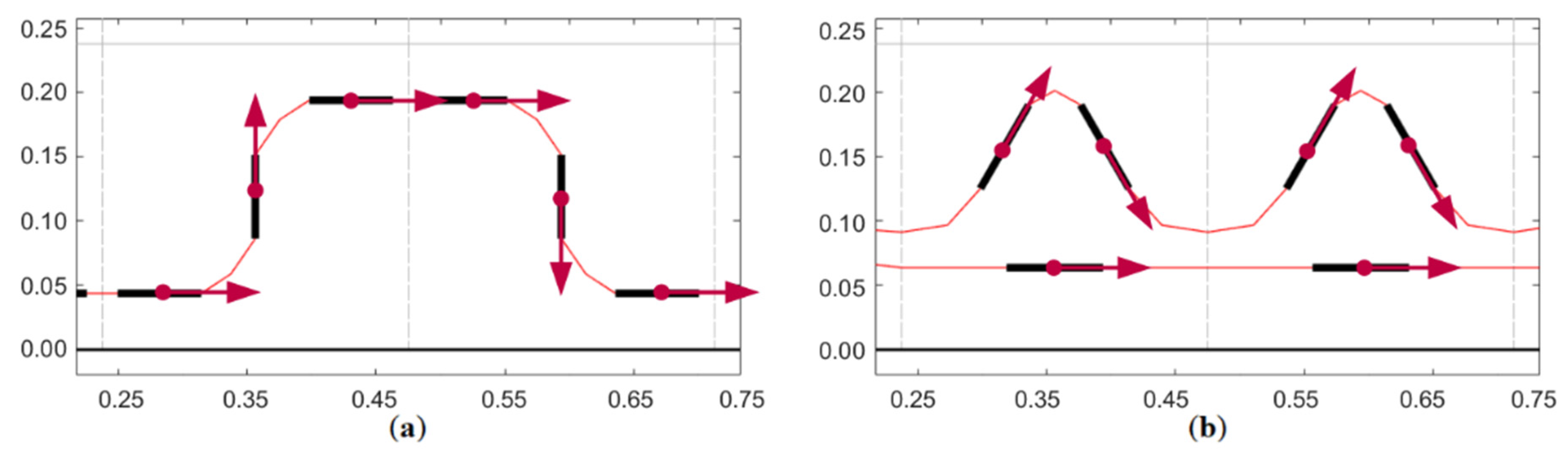
The SEA is a finite element (FE) based method that has been used as an FE post-processing tool for stress or strain ‘recovery’ (improved prediction) and error estimation. It is a variational based approach where the structural domain is discretized using smoothing elements. The problem is solved by minimizing a discrete least-squares error functional enforcing the continuity of the strains and their derivatives. Thus, the SEA recovers C1-continuous strains with C0-continuous derivatives. As the present work focused on a 1D formulation of the SEA, a two-node linear smoothing element with quadratic interpolation of strains and linear interpolation of the strain derivatives is used. The accuracy of the smoothed, SEA-generated strain data depended on the interpolation order of the smoothing element used and the complexity of the plate’s strain field. The SEA is expected to provide high accuracy results for an undamaged plate under uniform biaxial loading as the in-plane normal strains had uniform distributions, and the contribution of in-plane shear strain is negligible. For a damaged plate, recovering the strain field due to the crack is more challenging. In the presented context, however, the role of the SEA-based strain smoothing is to provide relatively accurate strain fields along the boundary of the plate. In addition to the in-situ measured strains, these smoothed strains would become input strains in the iFEM analysis.
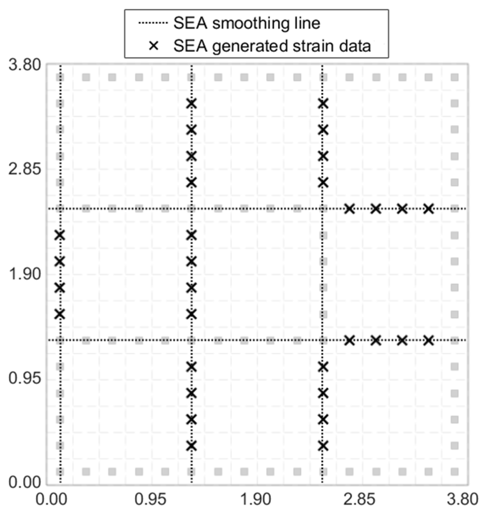
Figure 11 shows the use of the SEA on the strain data set of Unitcell-2. Along the grid lines, the SEA is used to interpolate existing FE strain data. Each grid line is discretized into a series of 1D smoothing elements, with at least one FE strain data point per element. The 1D SEA is used to smooth each in-plane strain component (
and
) individually. At the end of the smoothing procedure, each element of the grid would have tri-axial strain data at the element centroid. A similar SEA approach is used for Unitcell-1 as well. The use of fiber optics enabled strain measurements along long one-dimensional sensor paths, making it suitable for the 1D SEA methodology. However, different smoothing strategies, such as using 2D SEA elements or an alternate smoothing strategy, may also be used depending on the problem.
Note that Unitcell-1 lacked shear strain measurements, potentially leading to an inaccurate iFEM reconstruction. This issue is resolved by assuming a constant value of in-plane shear strain for all elements along the grid lines. A few additional strain rosettes are introduced in Configuration-1 to calculate shear strains at some discrete locations, and their average is used to represent the constant shear strain value for all elements along the grid lines. Although theoretically incorrect, this assumption is used to improve the quality of strain data available for the iFEM reconstruction. As the presented problem explored the plate cases under uniform biaxial loading, this assumption is expected to be moderately successful. However, in alternative problems involving more complex loading scenarios, the effect of in-plane shear strain would be more prominent, and this assumption would lead to erroneous results. The validity of this assumption will be discussed further when discussing the results in the following sections.
Different numerical integration strategies are employed for the iFEM analysis using strain data corresponding to the two Unitcells. As Unitcell-1 provided at most three strain measurement points within each element, the 3 × 3 Gauss scheme is used. In contrast, Unitcell-2 had only one measurement point within each element. Hence, the 2 × 2 Gauss scheme is used for Unitcell-2, with the same centroidal strain data used at all 4 Gauss points. This also led to an interesting investigation into using a constant set of strain data for integrating within an iQS4 element.
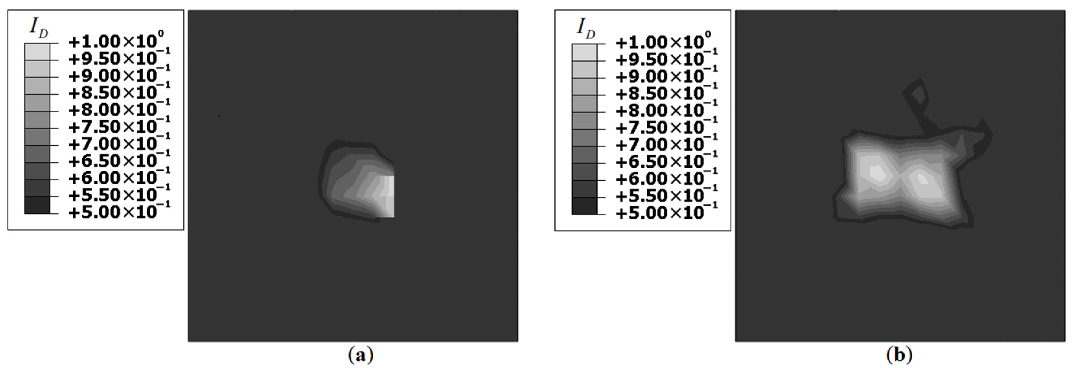
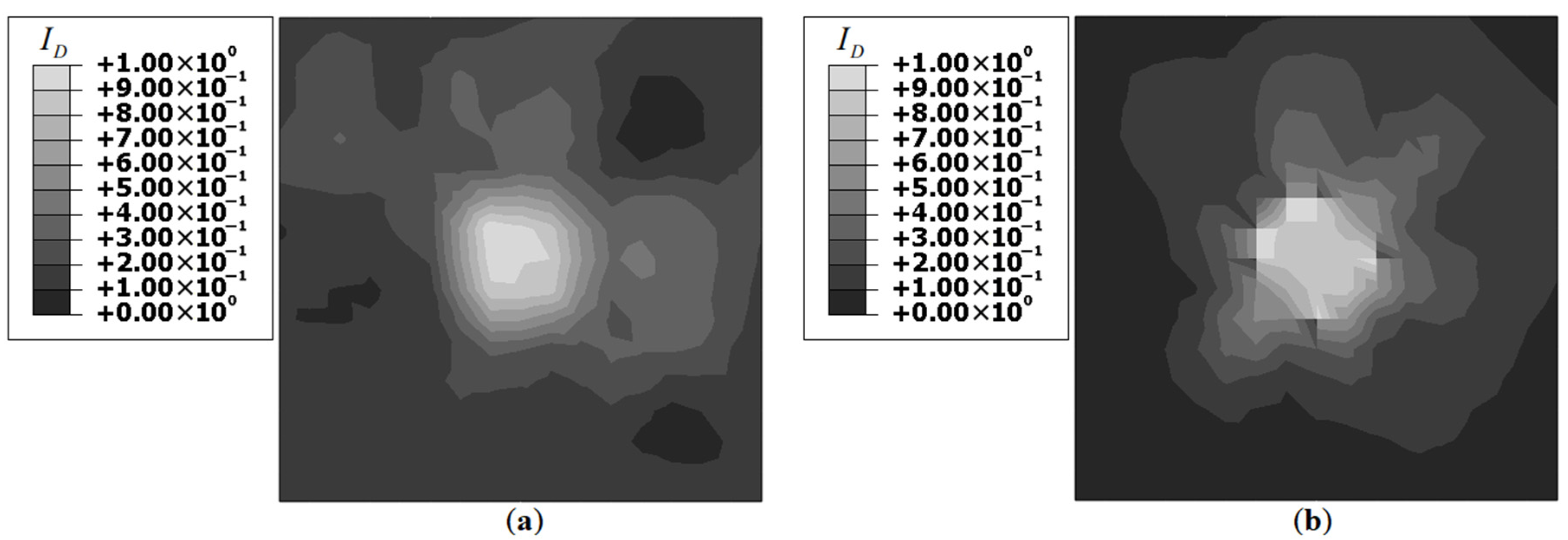
3.2.1. Results for Damage Case-1
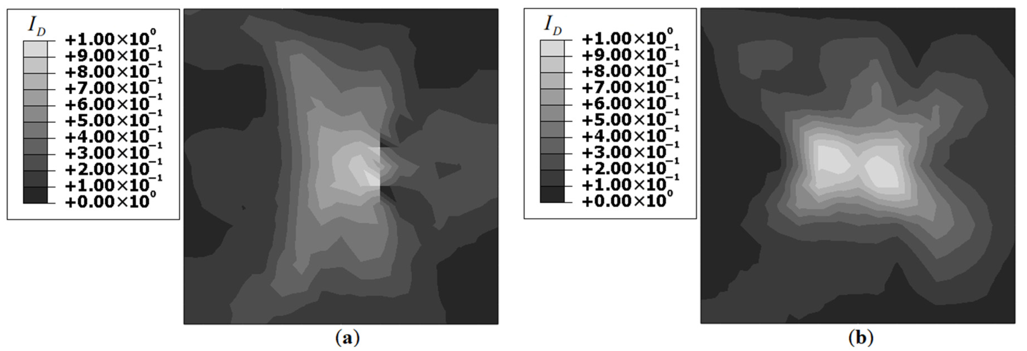
The iFEM results for Damage Case-1, using strain data corresponding to Unitcells-1 and 2 are shown in
Figure 12.
Results for Unitcell-2 are similar to the benchmark results, while Unitcell-1 results are deficient. Both plots showed a
concentration at the center of the plate; however, the results of Unitcell-1 are asymmetric. A greater
concentration is observed in the vicinity of those elements along which actual strain measurements are made using the optical fiber (see
Figure 12a). This asymmetry is not observed in the results of Unitcell-2. A comparison with the benchmark results revealed differences in the strain field distribution around the damage site. Compared to the benchmark results, the results of Unitcell-2 showed a greater dispersion of the damaged strain field to far-field locations. As the benchmark model used a greater number of strain-sensors along with a symmetric sensor grid, the results are symmetric with a well-defined strain peak at the center (see
Figure 5b). Despite these shortcomings, the plots of
Figure 12 offered sufficient information for successful damage detection.
Next, the effect of measurement noise on the results is investigated. The strain data is contaminated using random noise, added as a percentage of the strain magnitude. The noise distribution is based on a Gaussian curve with zero mean and the value of three standard deviations equal to 5%. The use of random noise in the measured strain data allowed for the introduction of various external factors that affected the method’s practical implementation. One key issue is the sensor bonding to the host structure [
37]. As the strain is transmitted from the host structure through the bonding surface (typically an epoxy adhesive) to the sensor, a strong and complete bond must be ensured for ideal strain transfer to the sensor and avoid any measurement errors. A similar issue is faced when fiber optic sensors are embedded within structures. Incorrect inclusion could lead to stress concentration between the structure and the sensor leading to erroneous measurements and potential damages to the host structure. Strain transfer analysis between the fiber cable, protective layer, bonding material, and the host structure [
38,
39] offers a way of identifying the parameters influencing the actual and measured strains and could be used for improving the strain measurements using fiber optic sensors. The current study adopted a more simplistic approach by using random noise to introduce these experimental effects in the numerical examples. The contour plots of
using contaminated strain data are shown in
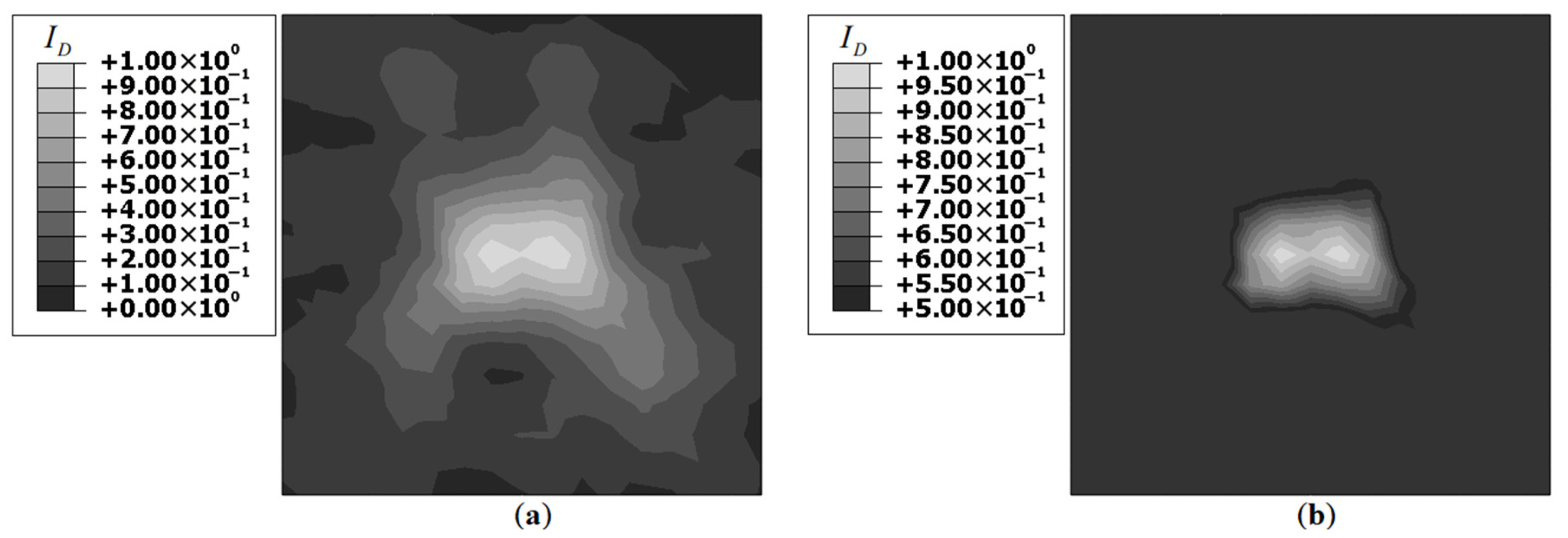
Figure 13.
Figure 13 shows that the introduction of noise lead to further diffusion of the strain field, with a prominent
peak at the center and smaller
peaks at far-field locations. This could be better illustrated using a
threshold of 0.5, i.e., the lower limit of the
plot is restricted to 0.5. The contour plots with this threshold level are shown in
Figure 14.
The use of a threshold helped to discriminate between regions with and without damage.
Figure 14 shows that the damage is located at the center of the plate. As discussed previously, asymmetry in
Figure 14a may lead to a false conclusion that the damage is not at the center but slightly off centric. Similarly, the dual peaks observed in
Figure 14b may also lead to a false interpretation of multiple damages present. Instead, these
distributions could be considered a feature of the method. These results are compared with benchmark iFEM results for Damage Case-1 using strain data contaminated with 5% noise and enforcing a threshold of 0.5 for isolating the damage location. These benchmark results are shown in
Figure 15. The threshold enforced
plot (
Figure 15b) depicted similar results to those of Unitcell-2 in terms of the distribution and location of the
peaks. Both cases showed the dual
peak at the center of the plate and no peaks at far-field locations. As demonstrated here, the use of a threshold to define a damage region rather than an exact point constituted an improved damage detection strategy for the present problem.
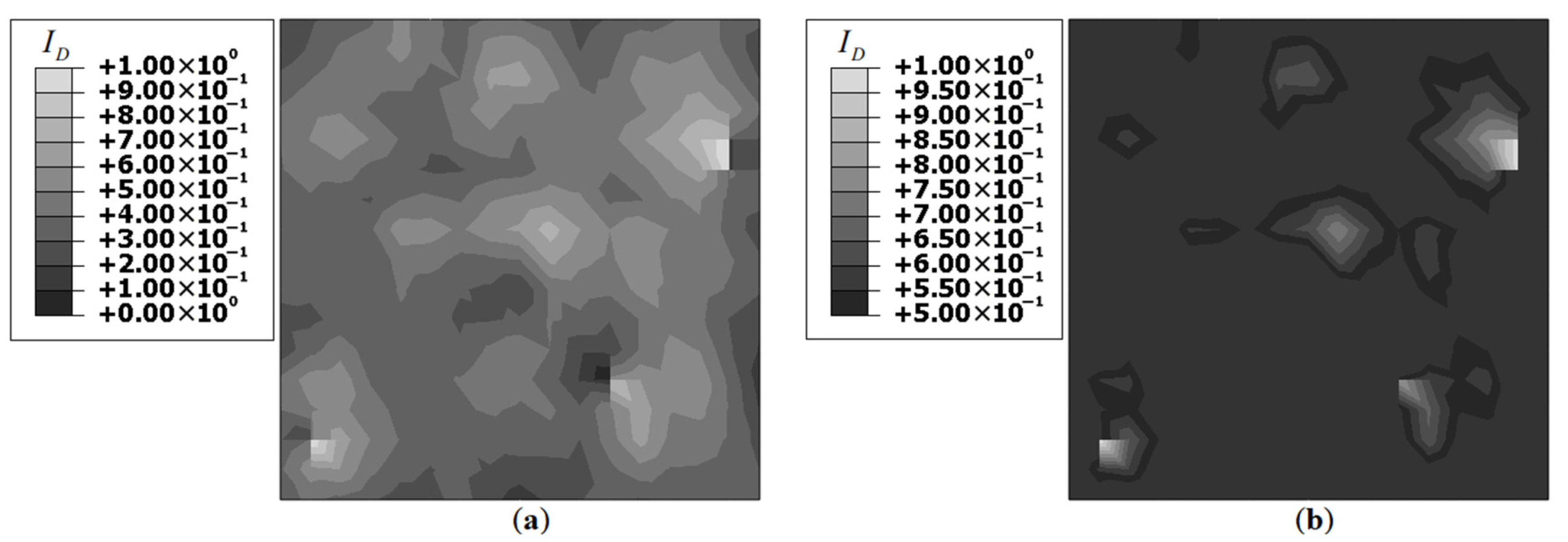
3.2.2. Results for Damage Case-2
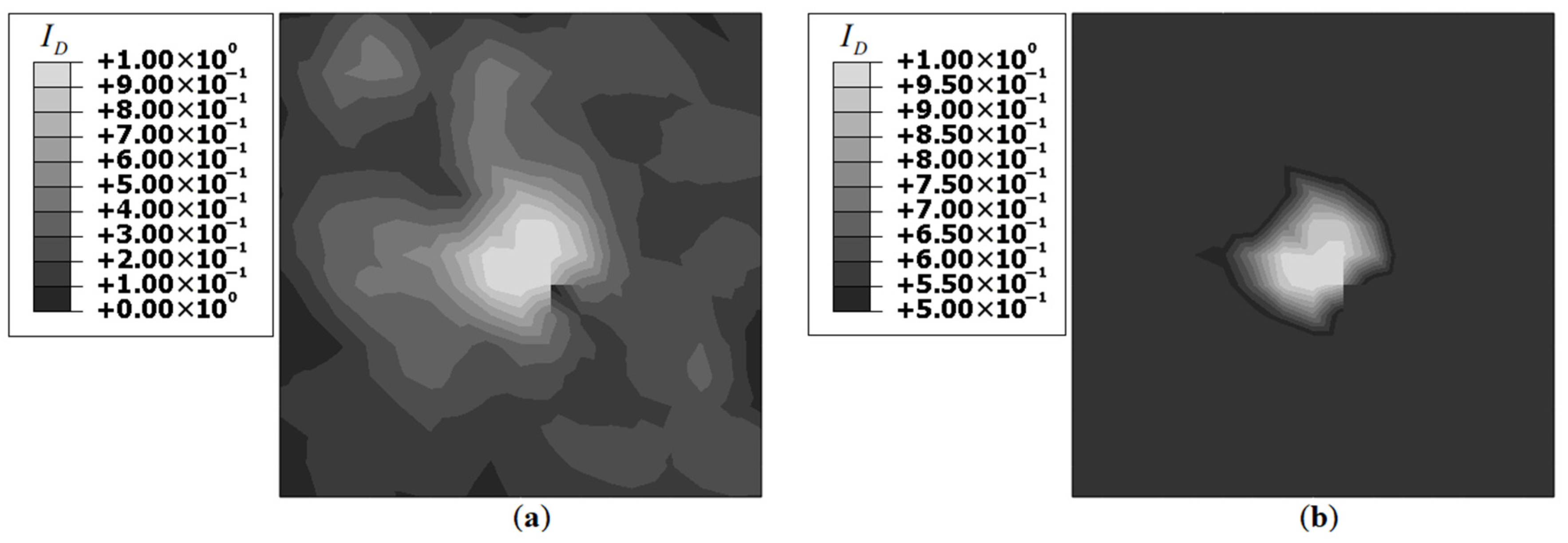
The iFEM results for Damage Case-2 are shown in
Figure 16. Despite the smaller damage size, the plots clearly showed a
peak near the actual damage site. Compared to the benchmark results (
Figure 6), the strain concentration is more diffuse; nevertheless, the plots illustrated the presence of damage near the corner of the plate. An interesting point to be noted is that even for Unitcell-2, the strain distribution far from the damage site is more prominent. This is not the case in the benchmark results where the far-field strains are virtually unaffected by the damage. The leakage of the strain field and subsequent contamination of the far-field strains are limitations of the Unitcell strategy. This illustrated potential difficulties in using the present strategy for detecting small-sized damages.
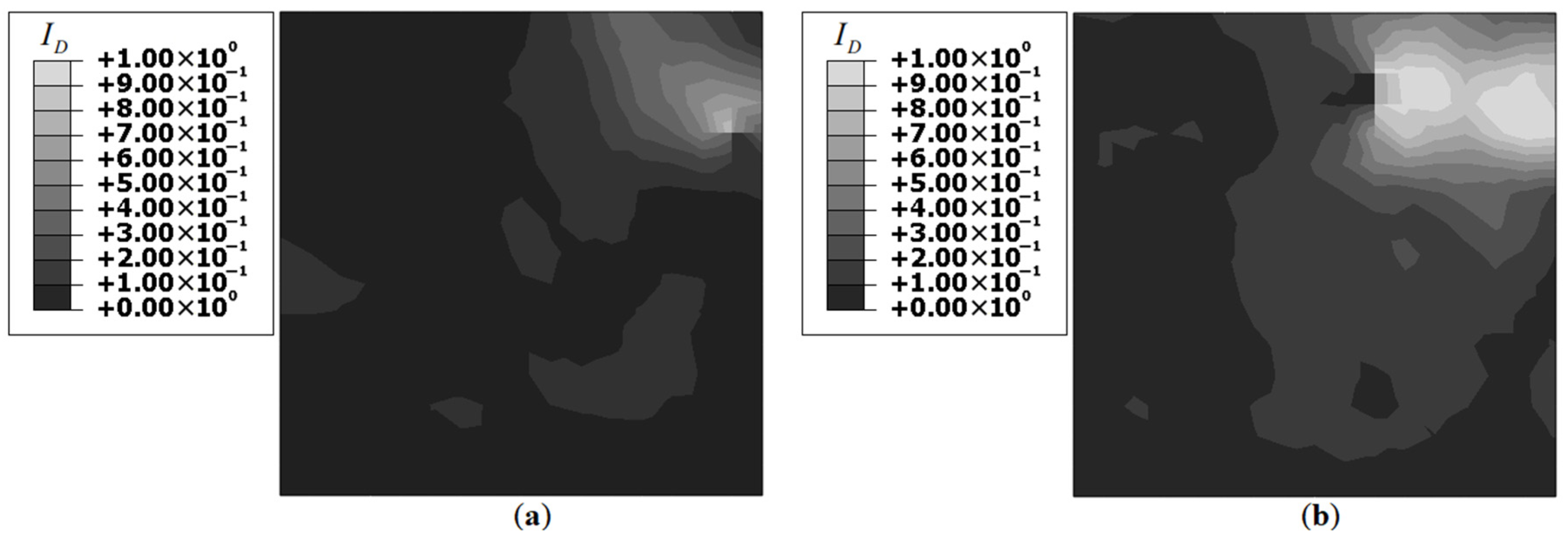
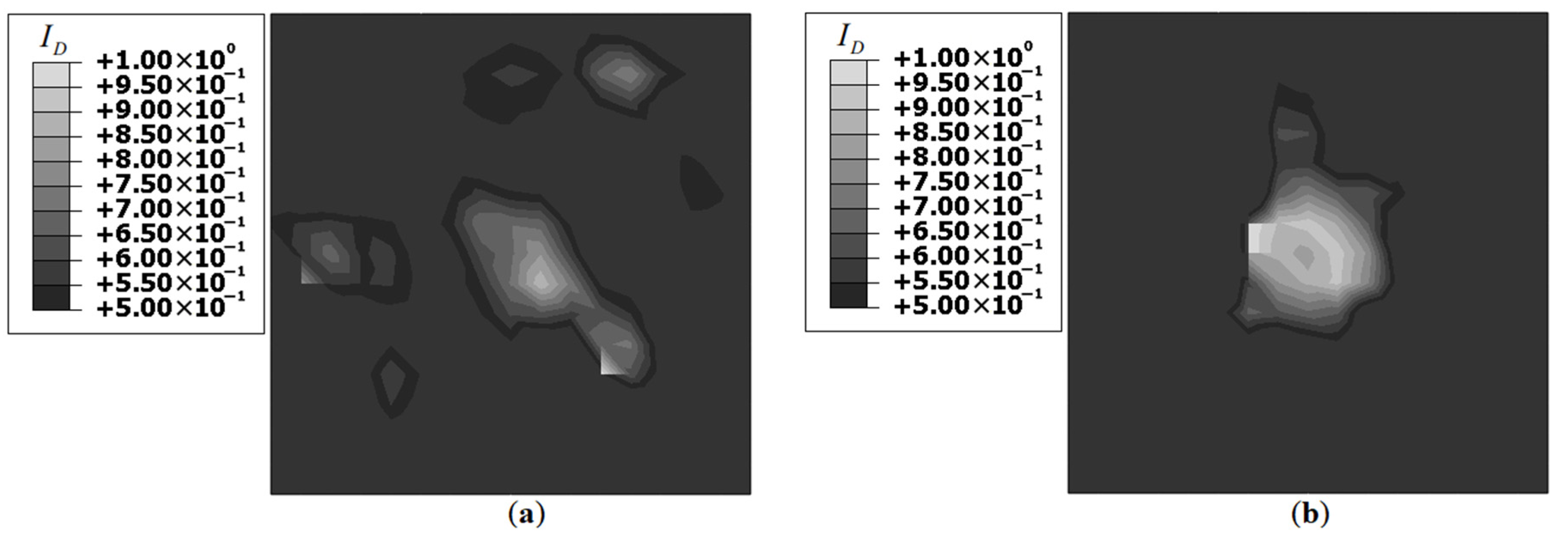
The iFEM results obtained using strain data contaminated with 5% noise are shown in
Figure 17.
The plots of
Figure 17 showed numerous
peaks at various locations of the plate. None of the peaks coincided with the actual damage site, leading to erroneous conclusions when used for damage detection. These results are compared with benchmark iFEM results for Damage Case-2 using contaminated strain data (5% noise). These benchmark results are shown in
Figure 18, and they also indicated a drop in damage detection performance due to the addition of noise. Compared to Unitcell-2, the benchmark results showed a prominent
peak near the damage site (
Figure 18b). The benchmark results also had the same limitations seen for Unitcell-2, where minor
peaks are seen at far-field locations. However, these results provided one significant inference: there is a lower limit to damage size that could be successfully detected using the proposed methodology. Successful damage detection is not possible as the strain perturbations due to the damage, measured by the strain-sensors, are smaller than the strain perturbations due to the added noise. It also pointed to possible alternative scenarios where similar-sized damages could be detected, e.g., when the damage is closer to one of the sensors and measures a higher strain perturbation.
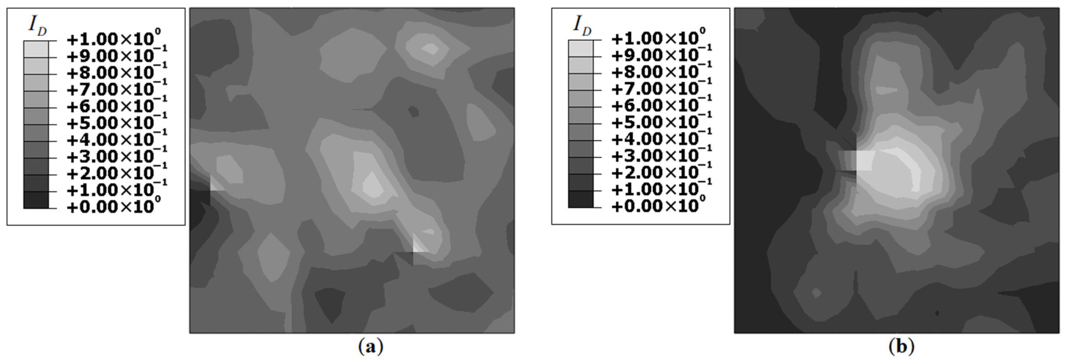
3.2.3. Results for Damage Case-3
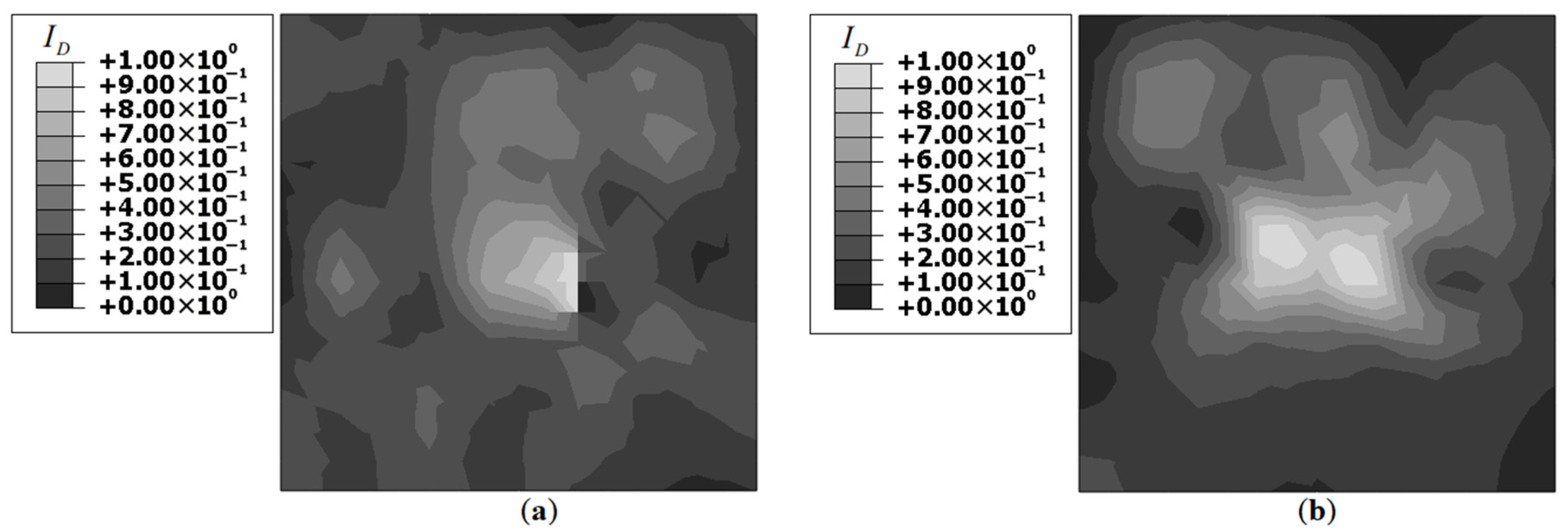
The iFEM results for Damage Case-3 are shown in
Figure 19. As seen in the benchmark results,
Figure 19 showed a
peak at the center of the plate and the damage orientation is reflected in the
distribution. Compared to the previous two cases, the results of Unitcell-2 are quite similar to the benchmark results, particularly in the regions around the damage and the strain distribution far away from the damage location.
Results of Unitcell-2 (
Figure 19b) showed a greater distribution of
perpendicular to the crack front. However, Unitcell-1 results are relatively symmetric, and no significant inference could be made regarding the damage orientation. The iFEM results obtained using strain data contaminated with 5% noise are shown in
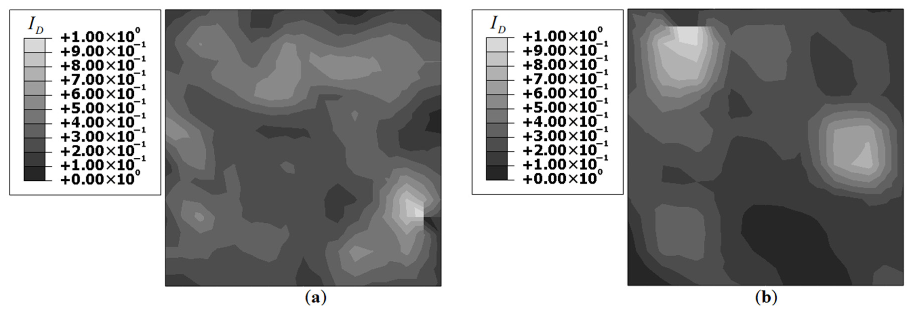
Figure 20.
The contour plots of
Figure 20 showed notable changes due to the addition of noise. Unitcell-1 results no longer presented an obvious damage location; however, improved predictions are obtained using Unitcell-2. These results are further refined using a threshold of 0.5; the corresponding plots are shown in
Figure 21. The use of a threshold showed multiple
peaks in the results of Unitcell-1, making accurate damage detection difficult. In contrast, the results of Unitcell-2 are of improved quality, with a well-defined
peak at the center. These results are again compared with the benchmark iFEM results for Damage Case-3 using strain data contaminated with 5% noise. The benchmark results are shown in
Figure 22. Compared to Unitcell-2, the benchmark results offered better directional information, with larger
distribution perpendicular to the crack front and a less diffuse strain field near the damage site. These results offer improved predictions of the crack position and orientation.
The superior predictions achieved with Unitcell-2 are attributed to its ability to provide the complete three strain component information within an element. Although the presented results focused on a relatively simple load case of a plate under biaxial loading, the real challenge is the strain field reconstruction near the damage site. Near the damage, the strain field distribution is complex, and the in-plane shear strain effect is significant. In this context, it is understandable that those sensor configurations with more in-plane shear strain measurements, i.e., the iFEM benchmark and Unitcell-2, yielded more accurate results. Although Unitcell-1 results are of theoretical interest, in most practical applications, the assumption of a constant in-plane shear strain over the plate is expected to produce somewhat erroneous results. In such situations, it would be of interest to investigate alternate configurations inspired by Unitcell-2.
Aside from the strain-sensor arrangement, the numerical integration scheme used and the smoothing strategy employed also influenced the iFEM accuracy. Both the 2 × 2 and 3 × 3 Gauss integration schemes are employed for the current set of results. Although an explicit claim regarding the superiority of one scheme over the other cannot be made, the accuracy of Unitcell-2 when using a constant set of centroidal strain data at all integration points of the 2 × 2 Gauss scheme is promising. This strategy reduced the number of strain measurement points required within an element, is more computationally efficient, and proved to be robust in the face of measurement noise. The choice of smoothing strategy also affected the iFEM results. Although the 1D smoothing strategy adopted in the present work produced good results, alternate strategies can also be explored and are expected to produce varying degrees of success. Regardless of the specific method considered, the relevant problem is the interpolation order of the smoothing strategy used and the complexity of the strain field investigated. A possible alternative is a 2D SEA scheme, where the plate is discretized using triangular smoothing elements. The refinement of the mesh could also be a contributing factor. The effect of the numerical integration scheme and the smoothing strategy employed are factors worthy of future investigation.
3.3. Damage Detection as a Function of Noise Level in Measured Strain Data
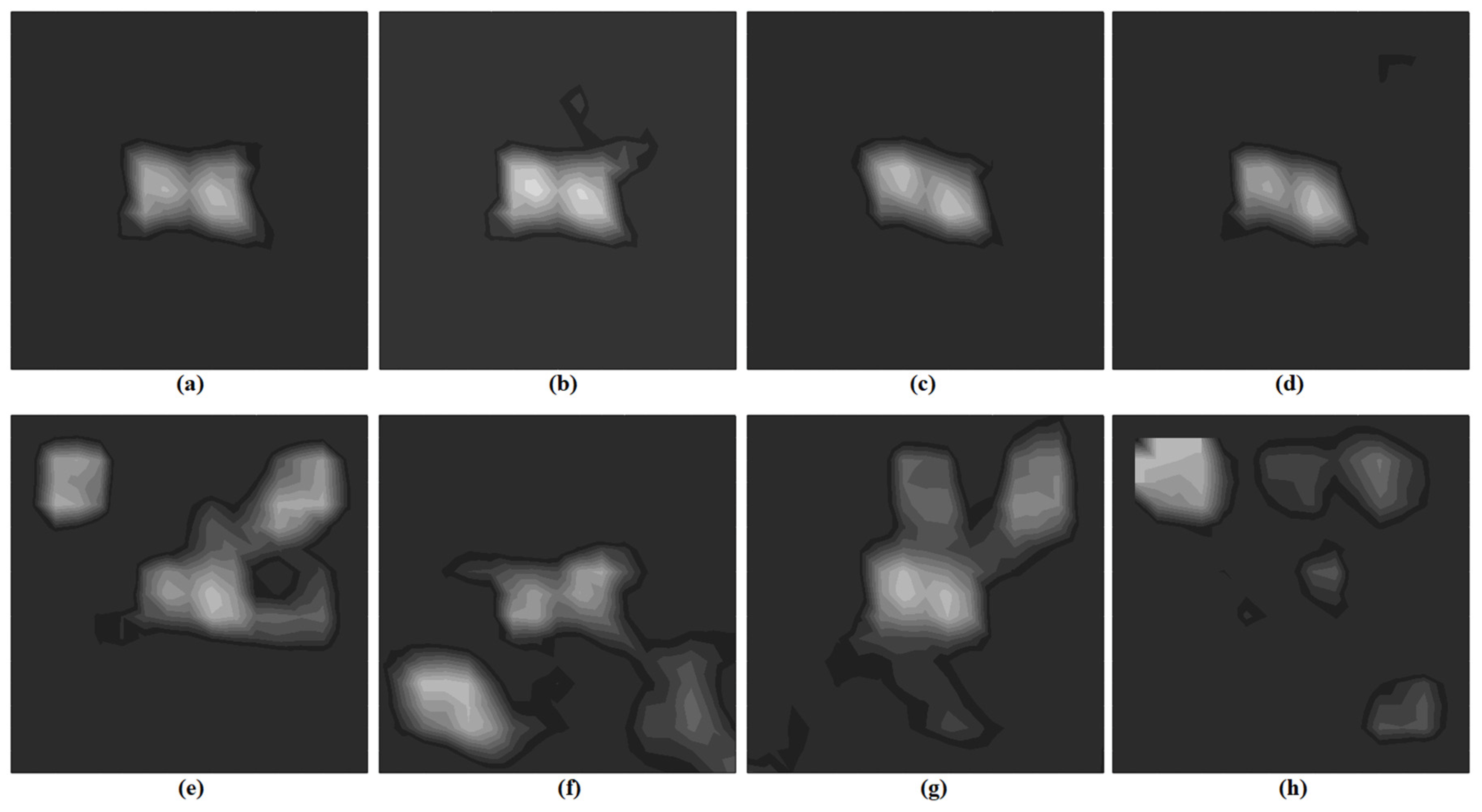
This section presents the results of a numerical study that explored the damage detection quality as a function of the noise level.
Section 3.2 reported iFEM results using strain data contaminated with 5% noise, where the two Unitcells reported a mixed level of success. The results of Unitcell-2 for Damage Cases-1 and 3 are successful in detecting damage and provided information regarding damage position and orientation. The effect of noise is further investigated here using Unitcell-2 strain data for reconstructing the strain field of Damage Case-1. The strain data is contaminated incrementally using eight different noise levels from 2.5% to 20%. The results of the study are presented as contour plots of
with a threshold of 0.5, and the plots are shown in
Figure 23.
The study results showed that successful damage detection is possible up to a noise level of 10%. For noise levels below 10%, the prominent peak is observed at the center of the plate, coinciding with the damage location. As the noise level increased further, additional peaks at far-field locations started to become more prominent. Even up to a noise level of 17.5%, it could be claimed that the prominent peak is at the center of the plate, and the use of a higher threshold could lead to successful damage detection by isolating the central peak. But that is no longer the case for noise levels of 20% or greater, as far-field peaks are dominant, and successful damage detection was no longer possible. The results further demonstrate the robustness of Unitcell-2 results in the presence of random noise and are promising for potential practical applications.


