Author Contributions
Conceptualization, N.M., D.G. and C.P.; Methodology, N.M., D.G. and C.P.; software, N.M.; validation, N.M., D.G. and C.P.; formal analysis, N.M. and C.P.; Investigation, N.M., D.G. and C.P.; Resources, D.G. and C.P.; Data Curation, N.M.; Writing, Original Draft Preparation, N.M.; Writing, Review and Editing, N.M., D.G. and C.P.; Visualization, N.M.; Supervision, N.M., D.G. and C.P. All authors have read and agreed to the published version of the manuscript.
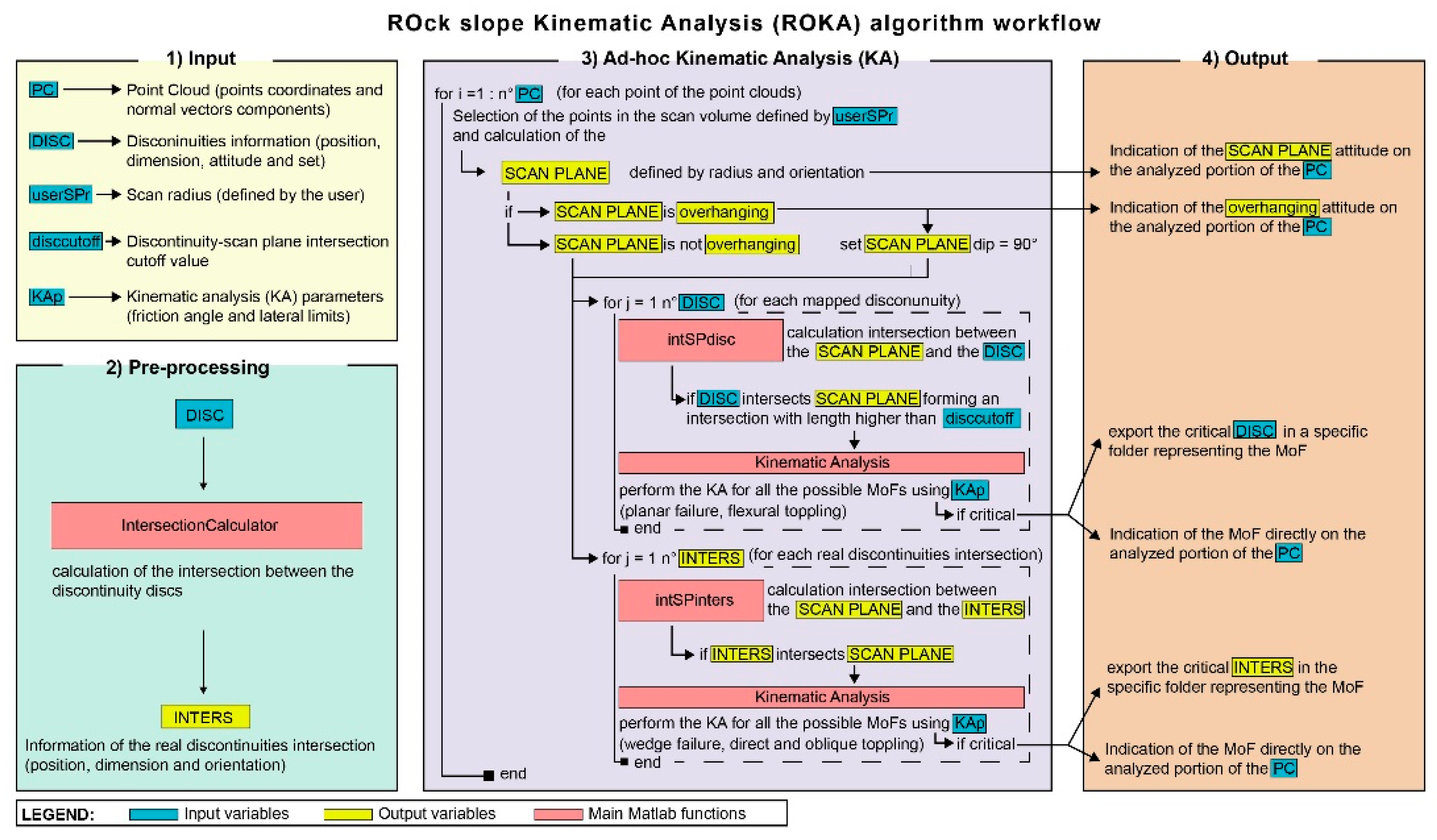
Figure 1.
Schematic representation of the workflow of the ROck slope Kinematic Analysis (ROKA) algorithm.
Figure 1.
Schematic representation of the workflow of the ROck slope Kinematic Analysis (ROKA) algorithm.
Figure 2.
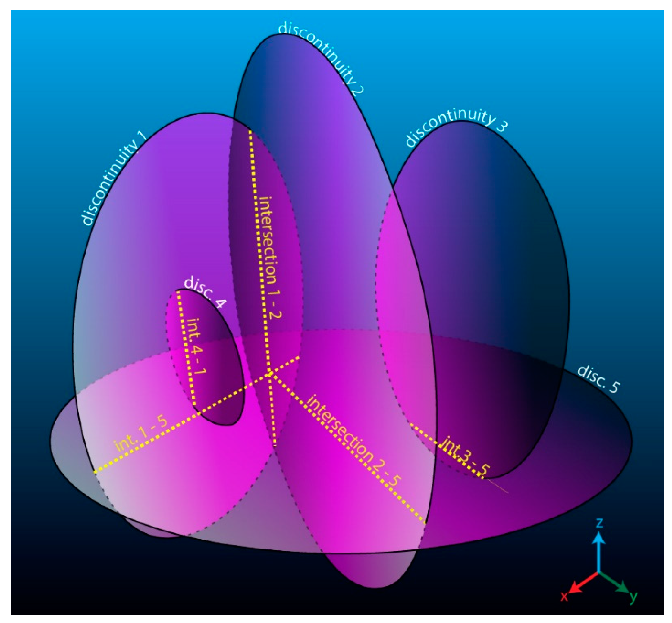
Representation of the Baecher’s disc model used to represent the discontinuity.
Figure 2.
Representation of the Baecher’s disc model used to represent the discontinuity.
Figure 3.
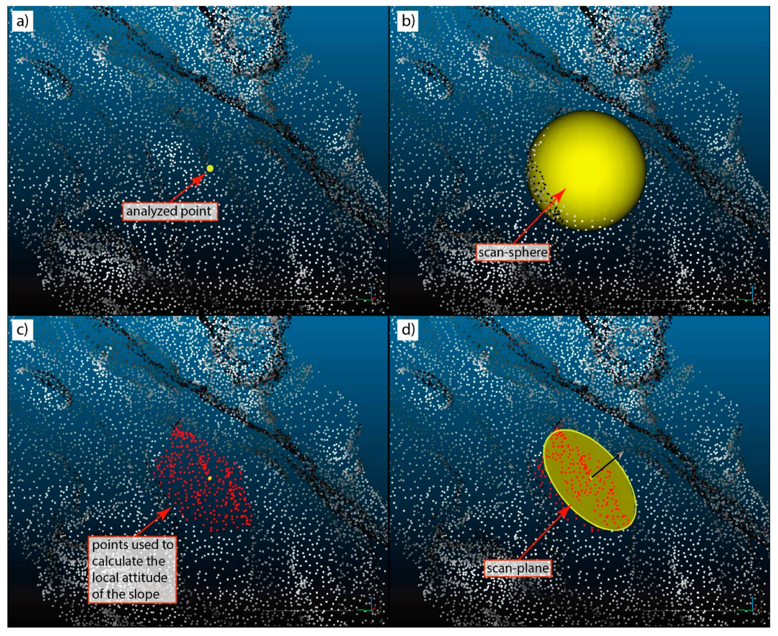
Example of the calculation influenced by the scan-radius. (a) For each point of the 3D point cloud, (b) a moving scan-sphere, with a scan-radius defined by the operator, (c) selects all the points used to calculate the local orientation of the slope. (d) A circular scan-plane, centered onto the analyzed point and oriented as the local portion of the slope (previously calculated using the scan-sphere), is defined. It will be used to verify if the discontinuity planes or intersections intersect the surface of the slope.
Figure 3.
Example of the calculation influenced by the scan-radius. (a) For each point of the 3D point cloud, (b) a moving scan-sphere, with a scan-radius defined by the operator, (c) selects all the points used to calculate the local orientation of the slope. (d) A circular scan-plane, centered onto the analyzed point and oriented as the local portion of the slope (previously calculated using the scan-sphere), is defined. It will be used to verify if the discontinuity planes or intersections intersect the surface of the slope.
Figure 4.
Example of the real intersection between the discontinuities represented by Baecher’s discs (modified after [
23]).
Figure 4.
Example of the real intersection between the discontinuities represented by Baecher’s discs (modified after [
23]).
Figure 5.
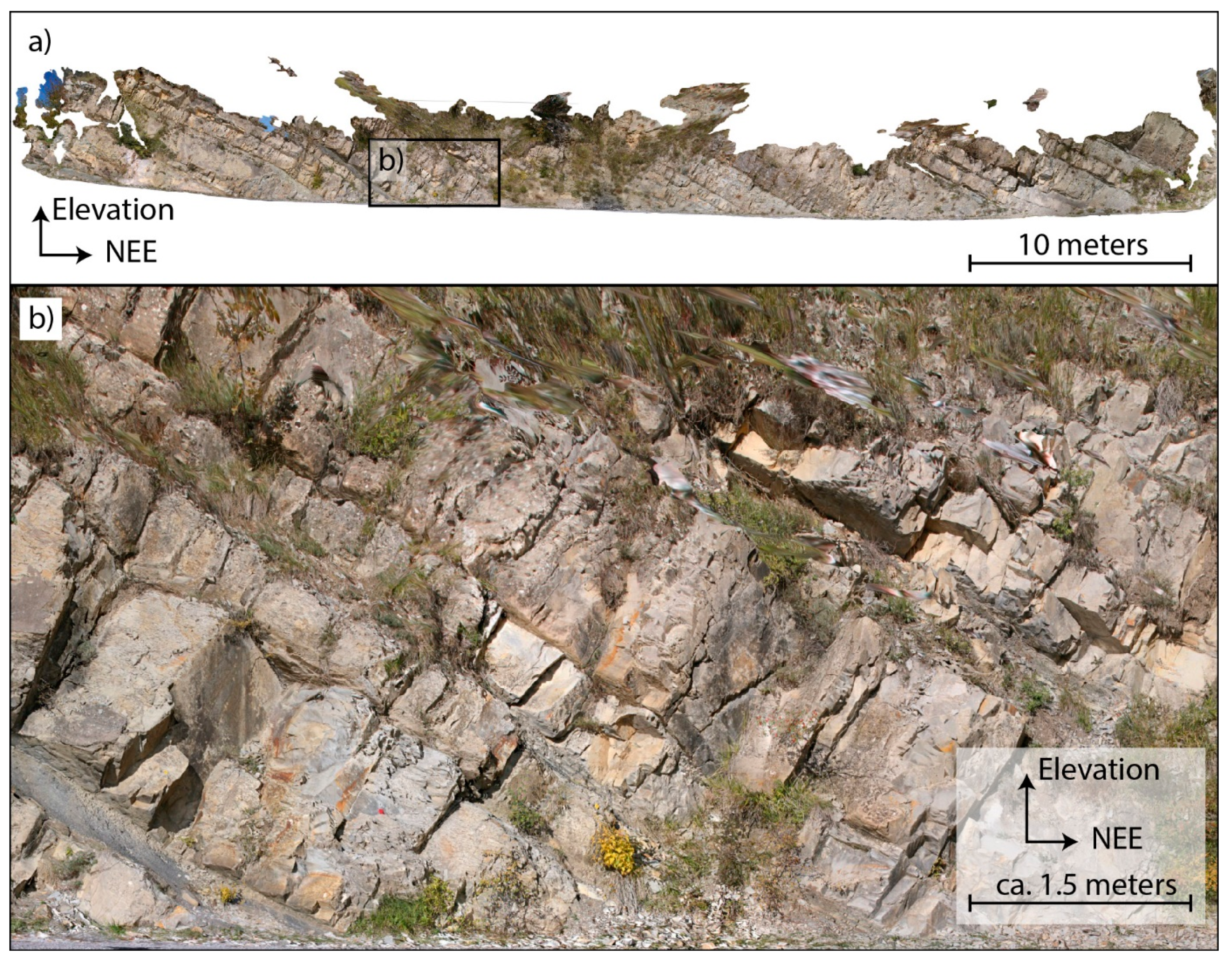
The study rock slope located along the upper Staffora Valley. The area delimited by the dashed yellow line indicates the portion of the outcrop investigated by Terrestrial Digital Photogrammetry.
Figure 5.
The study rock slope located along the upper Staffora Valley. The area delimited by the dashed yellow line indicates the portion of the outcrop investigated by Terrestrial Digital Photogrammetry.
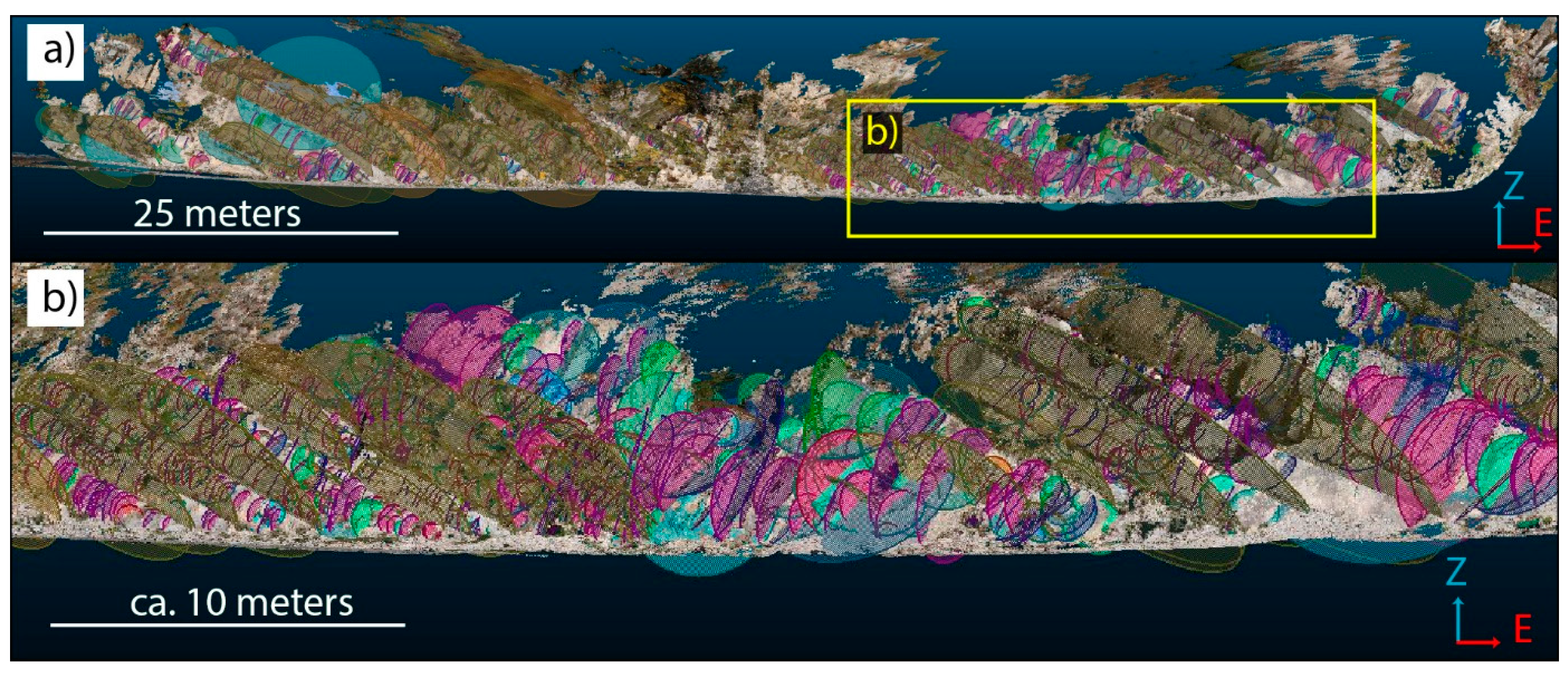
Figure 6.
(a) Three-dimensional (3D) model representing the outcrop acquired using the Terrestrial Digital Photogrammetry and (b) a detail of the 3D model. The visible discontinuities, bedding and fractures, delimitate unstable rock blocks. The abbreviation NEE means NorthEast-East
Figure 6.
(a) Three-dimensional (3D) model representing the outcrop acquired using the Terrestrial Digital Photogrammetry and (b) a detail of the 3D model. The visible discontinuities, bedding and fractures, delimitate unstable rock blocks. The abbreviation NEE means NorthEast-East
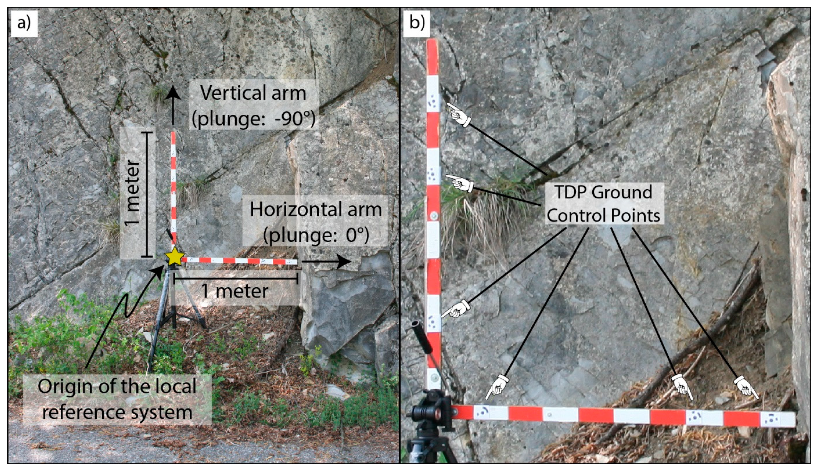
Figure 7.
(a) The L-shaped marker used to orient and scale the 3D model developed using the Terrestrial Digital Photogrammetry (TDP); (b) detail of the Ground Control Points (GCPs).
Figure 7.
(a) The L-shaped marker used to orient and scale the 3D model developed using the Terrestrial Digital Photogrammetry (TDP); (b) detail of the Ground Control Points (GCPs).
Figure 8.
(
a) The 3D discontinuities manually mapped onto the Digital Outcrop Model and (
b) a detail showing the circular-shape considered for the discontinuities following the Baecher’s disc model [
33].
Figure 8.
(
a) The 3D discontinuities manually mapped onto the Digital Outcrop Model and (
b) a detail showing the circular-shape considered for the discontinuities following the Baecher’s disc model [
33].
Figure 9.
Lower hemisphere projection and contour (Fisher distribution per 1% area) of the 1919 mapped discontinuities poles. The orientation (dip direction and dip) of the mean poles and planes of the five recognized sets are represented by the red dots and lines, respectively.
Figure 9.
Lower hemisphere projection and contour (Fisher distribution per 1% area) of the 1919 mapped discontinuities poles. The orientation (dip direction and dip) of the mean poles and planes of the five recognized sets are represented by the red dots and lines, respectively.
Figure 10.
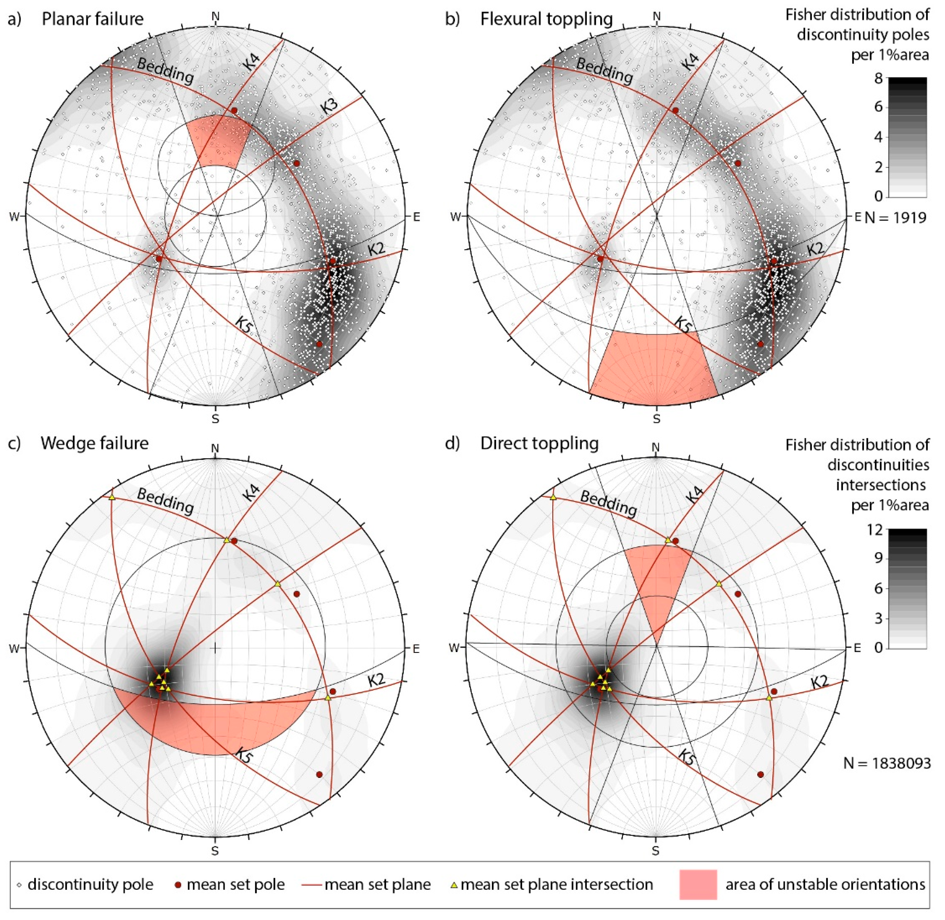
Traditional Kinematic Analysis (KA) of (a) planar failure, (b) flexural toppling, (c) wedge failure, and (d) direct toppling Modes of Failures (MOFs) performed onto a lower hemisphere and equal angle projection considering a mean slope attitude of 181°/56° (dip direction/dip), a friction angle of 30°, and the lateral limits in ± 20°. In the colored areas fall all the orientations of the critical discontinuities and their intersections.
Figure 10.
Traditional Kinematic Analysis (KA) of (a) planar failure, (b) flexural toppling, (c) wedge failure, and (d) direct toppling Modes of Failures (MOFs) performed onto a lower hemisphere and equal angle projection considering a mean slope attitude of 181°/56° (dip direction/dip), a friction angle of 30°, and the lateral limits in ± 20°. In the colored areas fall all the orientations of the critical discontinuities and their intersections.
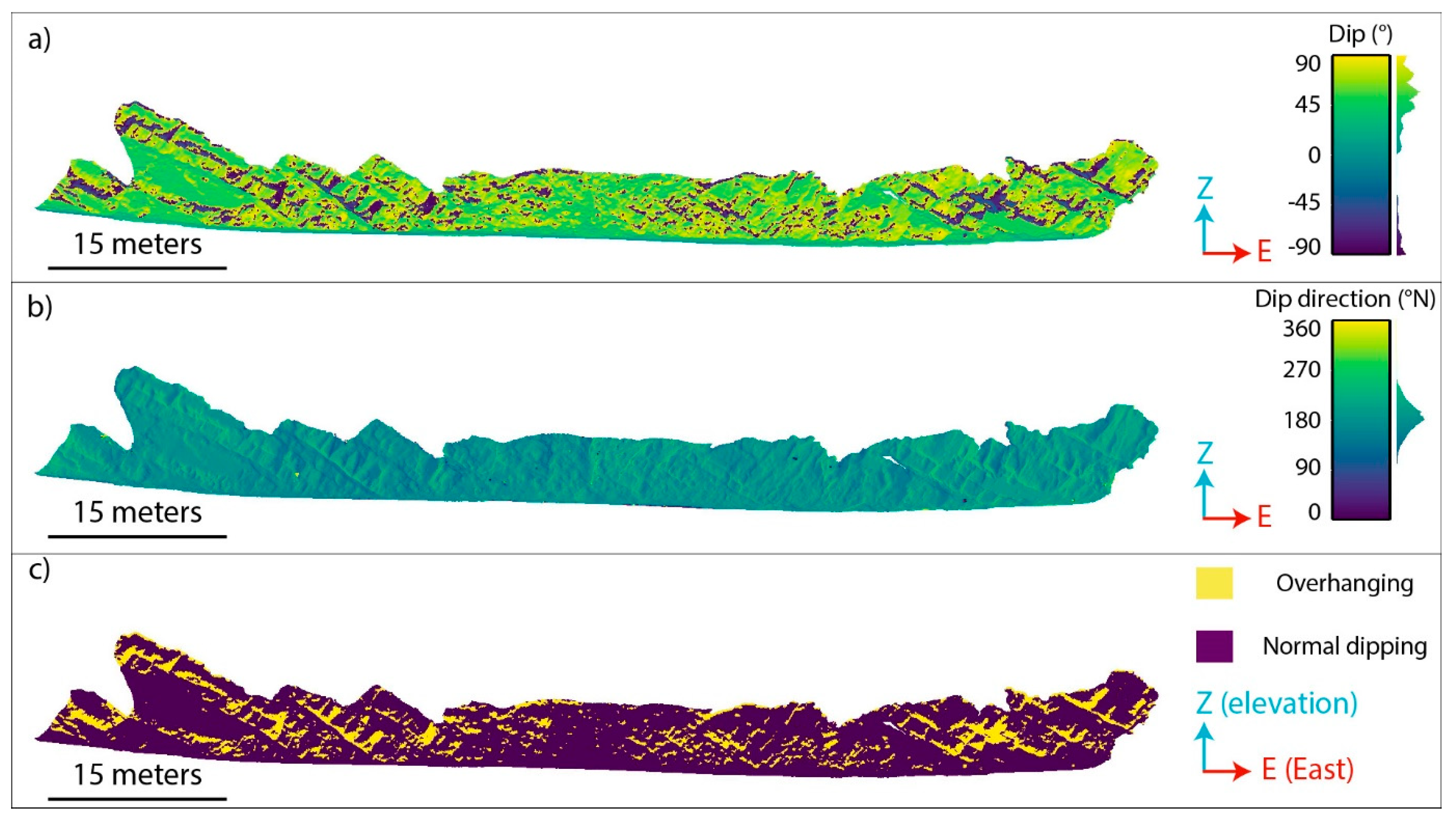
Figure 11.
The “local” orientation of the 3D model calculated from the normal vectors of the points that fall inside the moving scan-sphere, with a radius of 10 cm, is visualized as (a) dip and (b) dip direction. In (c), the areas in yellow represent portions of the slope that have an overhanging attitude.
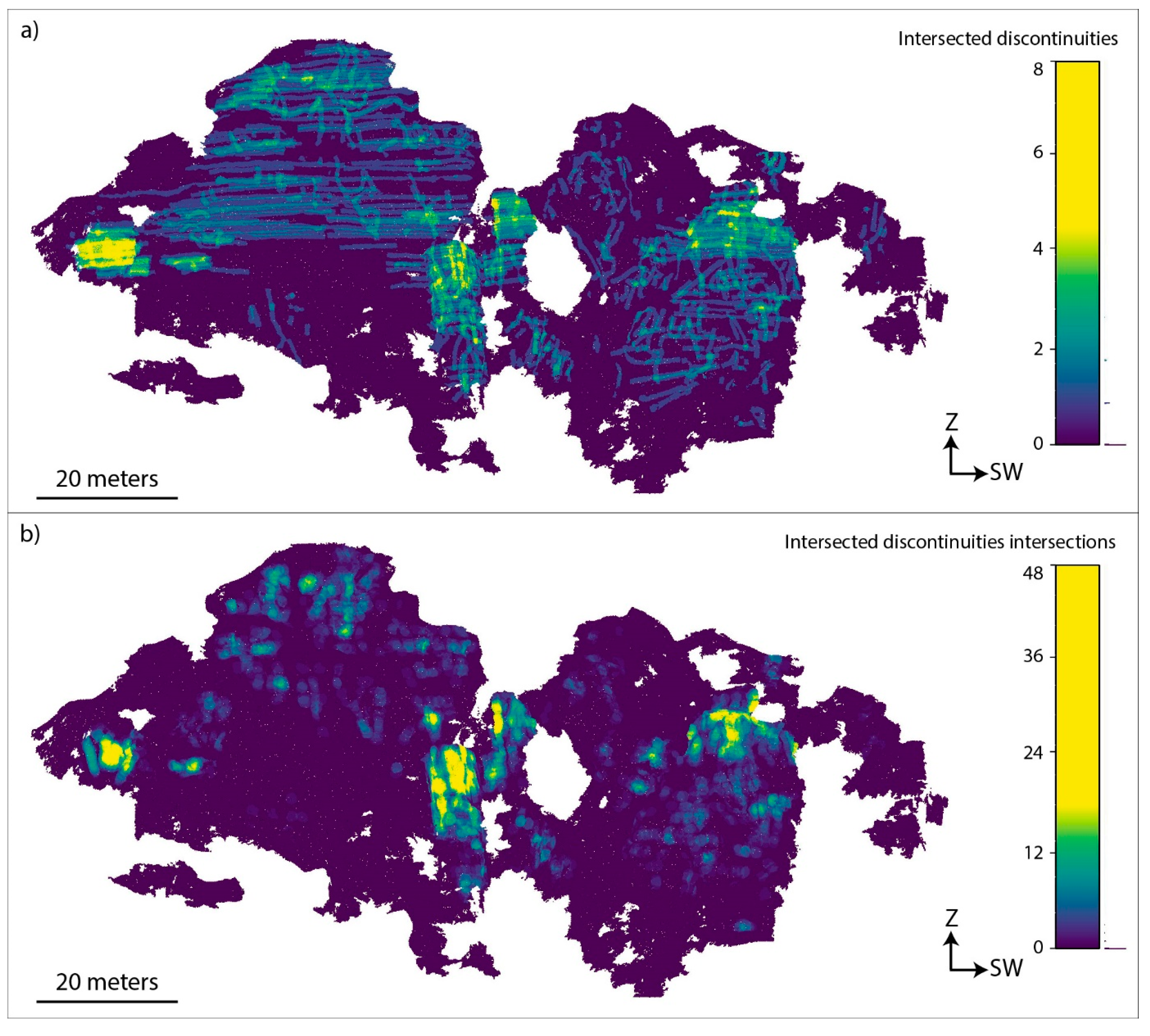
Figure 12.
Rendering of the 3D model of the slope indicating (
a) the number of the intersections between the scan-plane and discontinuities for every point of the cloud where the scan-plane (representing the local geometry of the slope) is centered, and (
b) the number of the intersections between the scan-plane and the discontinuity intersections. The middle of the outcrop shows no intersection because it is highly vegetated (see
Figure 6) and, therefore, no visible discontinuities were mapped (
Figure 8).
Figure 13.
Rendering of the 3D model indicating the results of the ROKA Kinematic Analysis (KA) of the possible Mode of Failure (MOF). The color scale represents the critical value of the discontinuity planes and intersections that could activate (
a) planar failure, (
b) flexural toppling, (
c) wedge failure, and (
d) direct toppling (see
Section 2.5 for the critical value definition).
Figure 14.
(
a) 3D discontinuities manually mapped onto the Digital Outcrop Model of the vertical rock cliff of Ormea [
23] and (
b) a detail of the preceding image. Al the discontinuities are represented by Baecher’s discs [
33].
Figure 14.
(
a) 3D discontinuities manually mapped onto the Digital Outcrop Model of the vertical rock cliff of Ormea [
23] and (
b) a detail of the preceding image. Al the discontinuities are represented by Baecher’s discs [
33].
Figure 15.
Lower hemisphere projection and contour (Fisher distribution per 1% area) of the poles of the 1036 mapped discontinuities. The orientations of the three recognized sets’ mean pole and plane values are represented by the red dots and lines, respectively, and the orientation is expressed in dip direction and dip.
Figure 16.
Traditional Kinematic Analysis (KA) of (a) planar failure, (b) flexural toppling, (c) wedge failure, and (d) direct toppling Modes of Failures (MOFs) performed onto a lower hemisphere and equal angle projection considering a mean slope attitude of 300°/75° (dip direction/dip). In the colored areas fall all the discontinuities and their intersections that could activate a specific MOF.
Figure 17.
(a) Dip and (b) dip direction of the local orientations of the 3D model of the slope calculated from the normal vectors of the points that fall inside the moving scan-sphere of a radius of 1 m. In (c), the areas in yellow represent portions of the slope that have an overhanging attitude.
Figure 17.
(a) Dip and (b) dip direction of the local orientations of the 3D model of the slope calculated from the normal vectors of the points that fall inside the moving scan-sphere of a radius of 1 m. In (c), the areas in yellow represent portions of the slope that have an overhanging attitude.
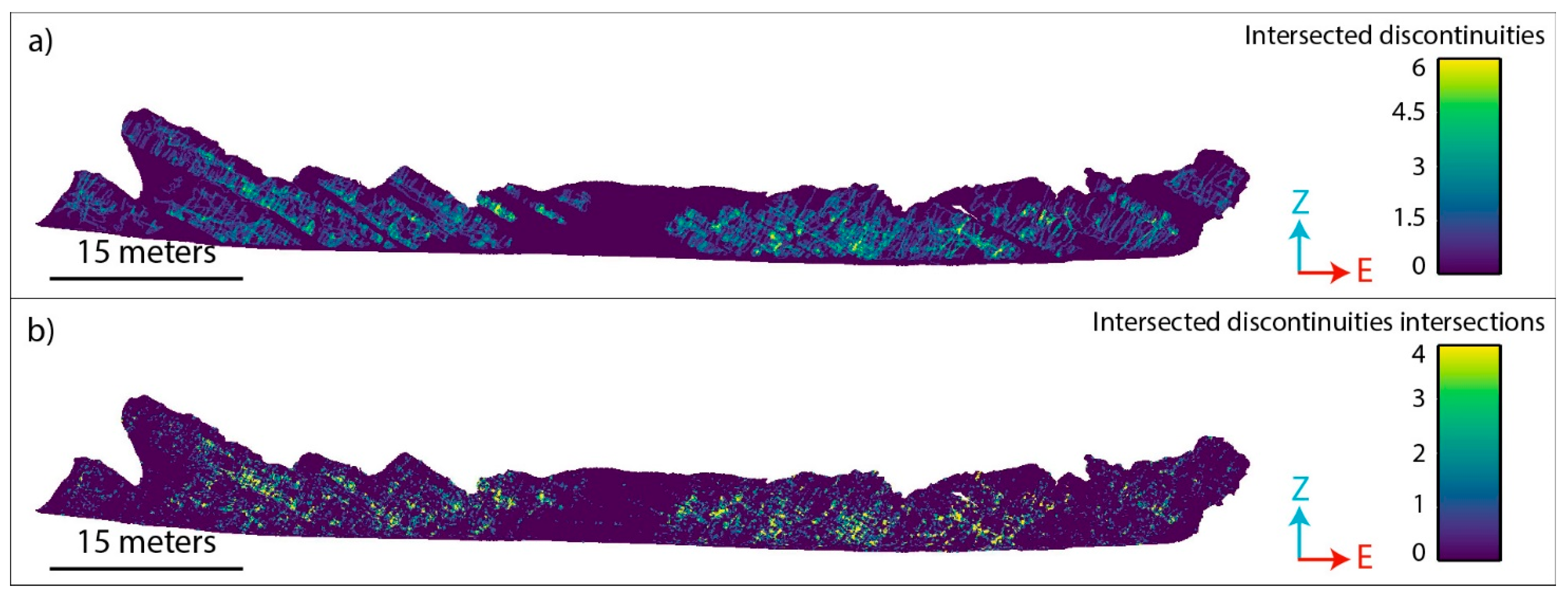
Figure 18.
Rendering of the 3D model of the slope indicating (a) the number of the intersections between the scan-plane and discontinuities for every point of the cloud where the scan-plane (representing the local geometry of the slope) is centered and (b) the number of the intersections between the scan-plane and the discontinuity intersections.
Figure 19.
Rendering of the 3D model indicating the results of the ROKA Kinematic Analysis of the possible modes of failure. The color scale represents the critical value of the discontinuity planes that could activate (
a) planar failure and (
b) flexural toppling (see
Section 2.5 for the critical value definition).
Figure 20.
Rendering of the 3D model indicating the results of the ROKA Kinematic Analysis of the possible modes of failure. The color scale represents the critical value of discontinuity intersections that could activate (
a) wedge failure and (
b) direct toppling, (see
Section 2.5 for the critical value definition).
Figure 21.
Lower hemisphere projection of the mean planes representing the slope used to perform the traditional Kinematic Analyses (KAs) and contour per 1% area of the poles indicating the slope’s local orientations in each point of the point clouds considered by ROKA algorithm. (a) Case study A and (b) case study B.
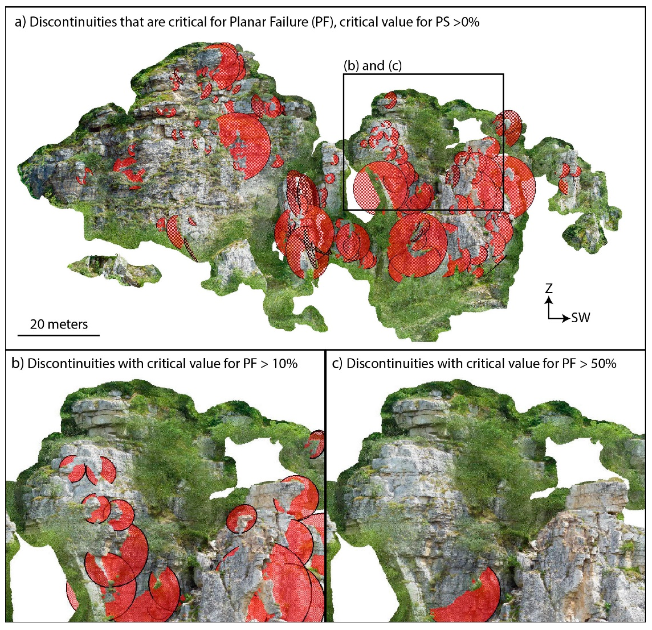
Figure 22.
(a) Identification of the critical parts of the slope for every specific MOF—the box identifies the sector presented in figures b and c—(b) visualization of the discontinuities that could activate the detected MOF and (c) their inspection and validation. In the figure, the ROKA algorithm results for planar failure MOF for case A are reported.
Figure 23.
(a) The ROKA algorithm allows the visualization and identification of the critical discontinuities for each MOF directly onto the 3D model of the rock slope—the box identifies the sector presented in figures b and c—and (b,c) to filter discontinuities considering their critical value based on the dimension of the intersection between the slope and the discontinuity.
Table 1.
Example of outfit of a XLSX file where the discontinuity geometry information is stored. The data reported in this table are rounded to fit well the text. The user can change the precision of the data as preferred.
Table 1.
Example of outfit of a XLSX file where the discontinuity geometry information is stored. The data reported in this table are rounded to fit well the text. The user can change the precision of the data as preferred.
| Dip | DipDirection | Radius | Xcenter | Ycenter | Zcenter | Nx | Ny | Nz |
|---|
| 83 | 119 | 2.56 | 67.66 | −46.94 | 845.85 | 0.86 | −0.48 | 0.11 |
| 75 | 327 | 3.01 | 67.94 | −45.74 | 847.04 | −0.51 | 0.82 | 0.24 |
| 85 | 287 | 2.35 | 67.95 | −46.30 | 846.46 | −0.94 | 0.30 | 0.07 |
| 86 | 284 | 1.08 | 67.49 | −46.55 | 847.56 | −0.96 | 0.2 | 0.06 |
| 11 | 108 | 18.16 | 101.61 | −26.32 | 891.34 | 0.19 | −0.06 | 0.97 |
Table 2.
According to the traditional Kinematic Analysis, the table shows the number of discontinuities that could activate the planar failure and flexural toppling modes of failure.
Table 2.
According to the traditional Kinematic Analysis, the table shows the number of discontinuities that could activate the planar failure and flexural toppling modes of failure.
| Discontinuity Set | Total Number of Discontinuities | Planar Failure | Flexural Toppling |
|---|
| K2 | 307 | 87 | 28% | 0 | 0% |
| K3 | 383 | 0 | 0% | 20 | 5% |
| Random | 176 | 0 | 0% | 6 | 3.4% |
| All sets | 1919 | 87 | 5% | 26 | 1% |
Table 3.
The table shows the number of discontinuities intersections that could activate the wedge failure and the direct toppling modes of failure according to the traditional Kinematic Analysis.
Table 3.
The table shows the number of discontinuities intersections that could activate the wedge failure and the direct toppling modes of failure according to the traditional Kinematic Analysis.
| Total Number of Critical Discontinuities | Wedge Failure | Direct Toppling |
|---|
| 1,838,093 | 202,196 | 77,411 |
| Percentages | 11% | 4% |
Table 4.
According to the ROKA Kinematic Analysis, the table shows the number of discontinuities that could activate planar failure and flexural toppling modes of failure.
Table 4.
According to the ROKA Kinematic Analysis, the table shows the number of discontinuities that could activate planar failure and flexural toppling modes of failure.
| Discontinuity Set | Considered Discontinuities | Planar Failure | Flexural Toppling |
|---|
| Bedding | 146 | 0 | 0% | 52 | 36% |
| K2 | 383 | 22 | 6% | 144 | 38% |
| K3 | 563 | 7 | 1% | 78 | 14% |
| K4 | 344 | 172 | 50% | 0 | 0% |
| K5 | 307 | 237 | 77% | 0 | 0% |
| Random set | 176 | 0 | 0% | 0 | 0% |
| All | 1919 | 438 | 23% | 278 | 14% |
Table 5.
According to the ROKA Kinematic Analysis, the table shows the number of discontinuities intersections that could activate wedge failure and direct toppling modes of failure.
Table 5.
According to the ROKA Kinematic Analysis, the table shows the number of discontinuities intersections that could activate wedge failure and direct toppling modes of failure.
| Total Number of Critical Discontinuities | Wedge Failure | Direct Toppling |
|---|
| 4349 | 1214 | 153 |
| Percentual | 28% | 4% |
Table 6.
According to the traditional Kinematic Analysis, the table shows the number of discontinuities that could activate planar and flexural toppling modes of failure. The bedding and K3 fracture set are not reported because their planes orientation does not suggest this possible failure.
Table 6.
According to the traditional Kinematic Analysis, the table shows the number of discontinuities that could activate planar and flexural toppling modes of failure. The bedding and K3 fracture set are not reported because their planes orientation does not suggest this possible failure.
| Discontinuity Set | Total Number of Discontinuities | Planar Failure | Flexural Toppling |
|---|
| K2 | 334 | 28 | 8% | 21 | 6% |
| Random | 340 | 24 | 7% | 22 | 6.5% |
| All | 1036 | 52 | 5% | 43 | 4% |
Table 7.
According to the traditional Kinematic Analysis, the table shows the number of discontinuities that could activate wedge and direct toppling modes of failure.
Table 7.
According to the traditional Kinematic Analysis, the table shows the number of discontinuities that could activate wedge and direct toppling modes of failure.
Total Number of Critical
Discontinuities Intersections | Wedge Failure | Direct Toppling |
|---|
| 564,373 | 73,536 | 14,007 |
| Percentages | 13% | 2% |
Table 8.
According to the ROKA Kinematic Analysis, the table shows the number of discontinuities that could activate planar and flexural toppling modes of failure.
Table 8.
According to the ROKA Kinematic Analysis, the table shows the number of discontinuities that could activate planar and flexural toppling modes of failure.
| Discontinuity Set | Considered Discontinuities | Planar Failure | Flexural Toppling |
|---|
| Bedding | 277 | 0 | 0% | 3 | 1% |
| K2 | 436 | 123 | 28% | 29 | 7% |
| K3 | 167 | 11 | 7% | 21 | 13% |
| Random set | 183 | 0 | 0% | 0 | 0% |
| All | 1063 | 134 | 13% | 53 | 5% |
Table 9.
According to the ROKA Kinematic Analysis, the table shows the number of discontinuities intersections that could activate wedge and direct toppling modes of failure.
Table 9.
According to the ROKA Kinematic Analysis, the table shows the number of discontinuities intersections that could activate wedge and direct toppling modes of failure.
| Total Number of Critical Discontinuities Intersections | Wedge Failure | Direct Toppling |
|---|
| 4667 | 538 | 710 |
| Percentual | 12% | 15% |
Table 10.
Comparison of the results of the different KA of wedge and direct toppling modes of failure.
Table 10.
Comparison of the results of the different KA of wedge and direct toppling modes of failure.
| Case of Study | Type of KA | Considered Discontinuities Intersections | Wedge Failure | Direct Toppling |
|---|
| Case A | Traditional | 1,838,093 | 202,196 | 11% | 74,411 | 4% |
| ROKA | 4349 | 1214 | 28% | 153 | 4% |
| Case B | Traditional | 564,373 | 73,536 | 13% | 14,007 | 2% |
| ROKA | 4667 | 538 | 12% | 710 | 15% |
Table 11.
Comparison of the results of the different KA of planar and flexural toppling modes of failure.
Table 11.
Comparison of the results of the different KA of planar and flexural toppling modes of failure.
| Case of Study | Type of KA | Considered Discontinuities | Planar Failure | Flexural Toppling |
|---|
| Case A | Traditional | 1919 | 87 | 5% | 26 | 1% |
| ROKA | 1919 | 438 | 23% | 278 | 14% |
| Case B | Traditional | 1036 | 52 | 5% | 43 | 4% |
| ROKA | 1063 | 134 | 13% | 53 | 5% |
Table 12.
Summary of the advantages and limitations of the ROKA algorithm.
Table 12.
Summary of the advantages and limitations of the ROKA algorithm.
| Advantages | Limitations |
|---|
- ✓
Only the “real” intersections between the 3D mapped discontinuities are considered, evaluating their effective position, orientation, and dimension ( Figure 4); - ✓
All the “real” orientations of the slope are calculated, using a scan-sphere ( Figure 3), and these local attitudes are used to perform the KA only when a discontinuity, or two discontinuities that form a wedge, intersect the local portion of the slope; - ✓
The KA can be validated by visualizing the results onto the 3D model of the rock slope ( Figure 22); - ✓
The critical discontinuities can be located in the 3D space and classified according to the extent of their intersection with the slope ( Figure 23), giving great help to the user that must perform the stability analysis
| - ✕
The Baecher’s disc model considered by ROKA can lead to miscalculation of the possible dimensions and positions of the discontinuities intersections (wedge) due to the presence of discontinuities of different shapes; - ✕
Pitfalls of the remote sensing technique used to build the slope 3D model (e.g., unsatisfying resolutions or occlusion effects) can cause inaccuracies in the detection and mapping of the discontinuities; - ✕
The possible modes of failure (planar failure, wedge failure, flexural toppling, and direct toppling) are determined considering only the discontinuities and slope orientations, without considering other important features as aperture, roughness, filling, and seepages of the discontinuities.
|


