Article

Aerodynamic Design Optimization of a Morphing Leading Edge and Trailing Edge Airfoil–Application on the UAS-S45

Research Laboratory in Active Controls, Avionics and Aeroservoelasticity (LARCASE), Université du Québec, École de Technolgie Supérieure, 1100 Notre-Dame West, Montreal, QC H3C1K3, Canada
*
Author to whom correspondence should be addressed.
Appl. Sci. 2021, 11(4), 1664; https://doi.org/10.3390/app11041664
Submission received: 10 December 2020 / Revised: 3 February 2021 / Accepted: 6 February 2021 / Published: 12 February 2021
(This article belongs to the Special Issue Aircraft Modeling and Simulation)

Abstract

:
This work presents an aerodynamic optimization method for a Droop Nose Leading Edge (DNLE) and Morphing Trailing Edge (MTE) of a UAS-S45 root airfoil by using Bezier-PARSEC parameterization. The method is performed using a hybrid optimization technique based on a Particle Swarm Optimization (PSO) algorithm combined with a Pattern Search algorithm. This is needed to provide an efficient exploitation of the potential configurations obtained by the PSO algorithm. The drag minimization and the endurance maximization were investigated for these configurations individually as two single-objective optimization functions. The aerodynamic calculations in the optimization framework were performed using the XFOIL solver with flow transition estimation criteria, and these results were next validated with a Computational Fluid Dynamics solver using the Transition γ R e θ Shear Stress Transport (SST) turbulence model. The optimization was conducted at different flight conditions. Both the DNLE and MTE optimized airfoils showed a significant improvement in the overall aerodynamic performance, and MTE airfoils increased the efficiency of CL3/2/CD by 10.25%, indicating better endurance performance. Therefore, both DNLE and MTE configurations show promising results in enhancing the aerodynamic efficiency of the UAS-S45 airfoil.

1. Introduction

1.1. Outline of the Research

The goal of reducing global fuel consumption and fuel-related emissions has placed tremendous pressure on the aviation industry. In 2018, the aviation industry was responsible for 895 million tons of CO2 emissions globally emitted into the atmosphere [1]. Reducing fuel consumption will benefit both the world environment and the air transport industry. According to the Aviation Transport Action Group (ATAG), a reduction in fuel burning will have a significant impact on the aviation industry because the largest operating cost of this industry is fuel [1]. Drastic measures are still required even though some steps have already been taken to reduce these emissions. Various solutions have been implemented by the aviation industry, including smart material technology, laminar flow technology, air traffic management technologies, advanced propulsion techniques and sustainable fuels [2,3,4]. Morphing wing technology is one of the technologies showing high potential in decreasing aircraft fuel consumption [5,6,7,8]. Even though there is no settled definition for “morphing”, this term is borrowed in Aviation Technology from avian flight to describe the ability to modify maneuvers at certain flight characteristics in order to obtain the best possible performance. This type of application requires morphing structures capable of adapting to changing flight conditions. Morphing systems include several wing shape modifications, span or sweep changes, changes in twist or dihedral angle [9] and variations of the airfoil camber [7] or of the thickness distribution [4]. In the design phase, both military and civilian aircraft traditionally fly at a single or few optimum flight conditions; morphing, however, is envisioned to increase the number of optimum operational points for a given aircraft [5].
The morphing strategy scope is broad in the sense that an optimal solution can be generated in various ways with respect to a wide spectrum of mission profiles and types, and flight regimes. Novel technologies need to be part of recent efforts to produce environmentally sustainable and efficient aircraft. To meet environmental guidelines, including those of the International Civil Aviation Organization’s (ICAO’s) Committee on Aviation Environmental Protection (CAEP), innovative technologies such as “morphing” are fascinating as they provide advantages over conventional wing configurations [10]. Additionally, “morphing” is more practically applied in Unmanned Aerial Vehicles (UAVs) because of their reduced scale and lower complexity in terms of wing design structure and energy consumption expressed in terms of actuation power [6,11,
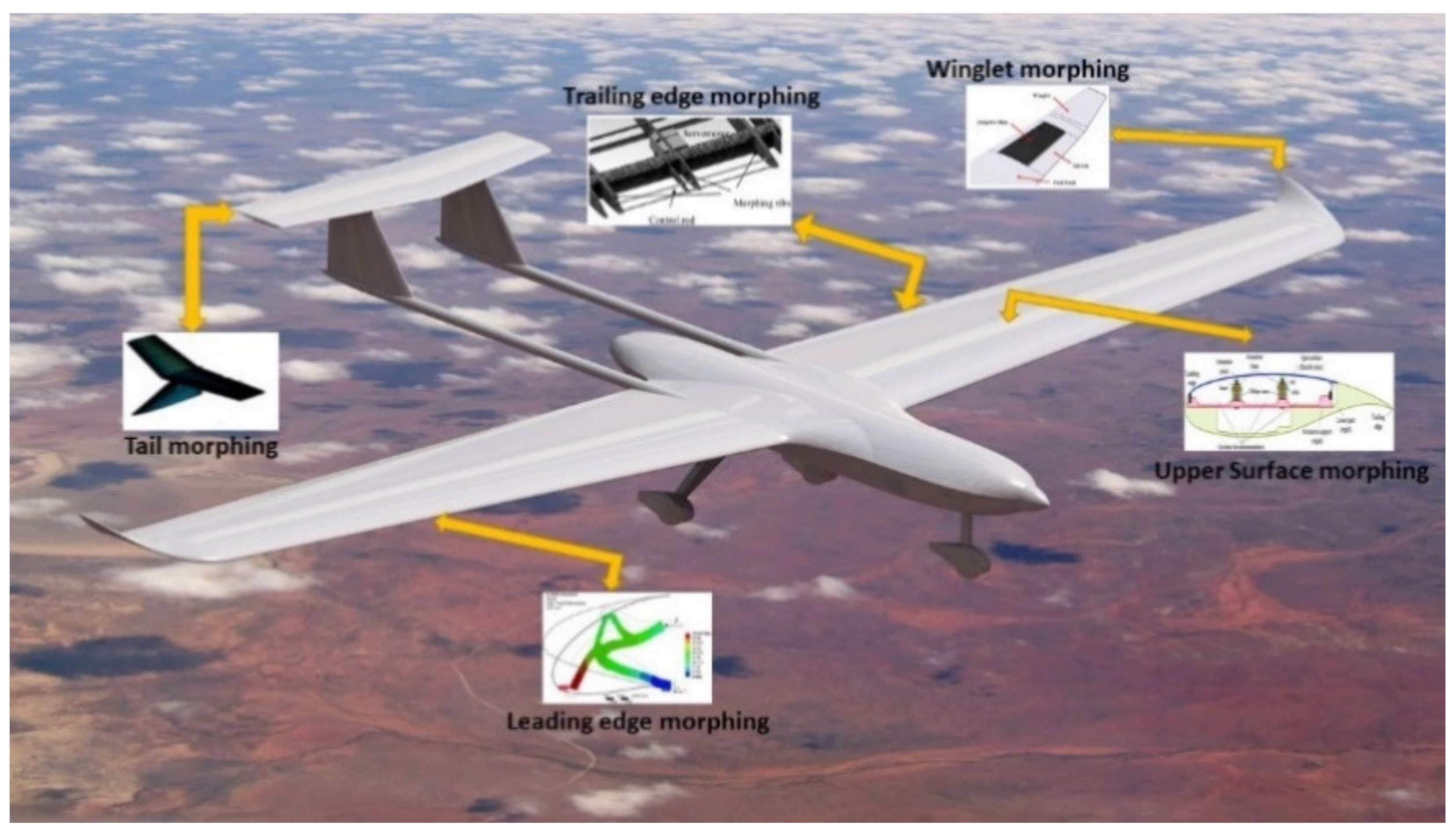
12], in addition to the advantages that morphing designs are lighter and less noisy than their conventional designs. Some morphing opportunities with potential benefits for increasing aerodynamic performance of the UAS-S45 are shown in Figure 1.
Aircraft are designed to achieve optimal aerodynamic performance (maximum lift-to-drag ratio) for a mission specification and for an extended range of flight conditions. Nevertheless, these mission specifications change continuously throughout the different flight phases, and an aircraft often flies at non-optimal flight conditions. Although the conventional hinged high lifting devices and trailing edge surfaces (discrete control surfaces) in aircraft are effective in controlling the airflow for different flight conditions, they create surface discontinuities, which increase the drag [13,14]. The disadvantages of these hinged surfaces are found in both their deployed and retracted configurations [15]. When deployed, the gaps between the high lifting surface and the wing can cause noise and turbulence, and therefore can produce a turbulent boundary layer and thus increase drag. Even when retracted, the trailing edge hinges still produce a turbulent boundary layer. Numerous researchers believe that the laminar flow technology has the maximum potential to reduce drag and to avoid flow separation [16,17]. For this goal, the wings require the design of thin airfoils, seamless high-quality surfaces and variable droop leading edges. The use of these high continuous smooth lifting devices in UAVs will further broaden their flight envelope and extend their endurance. These challenges can be addressed by using morphing technology in the current aviation industry.
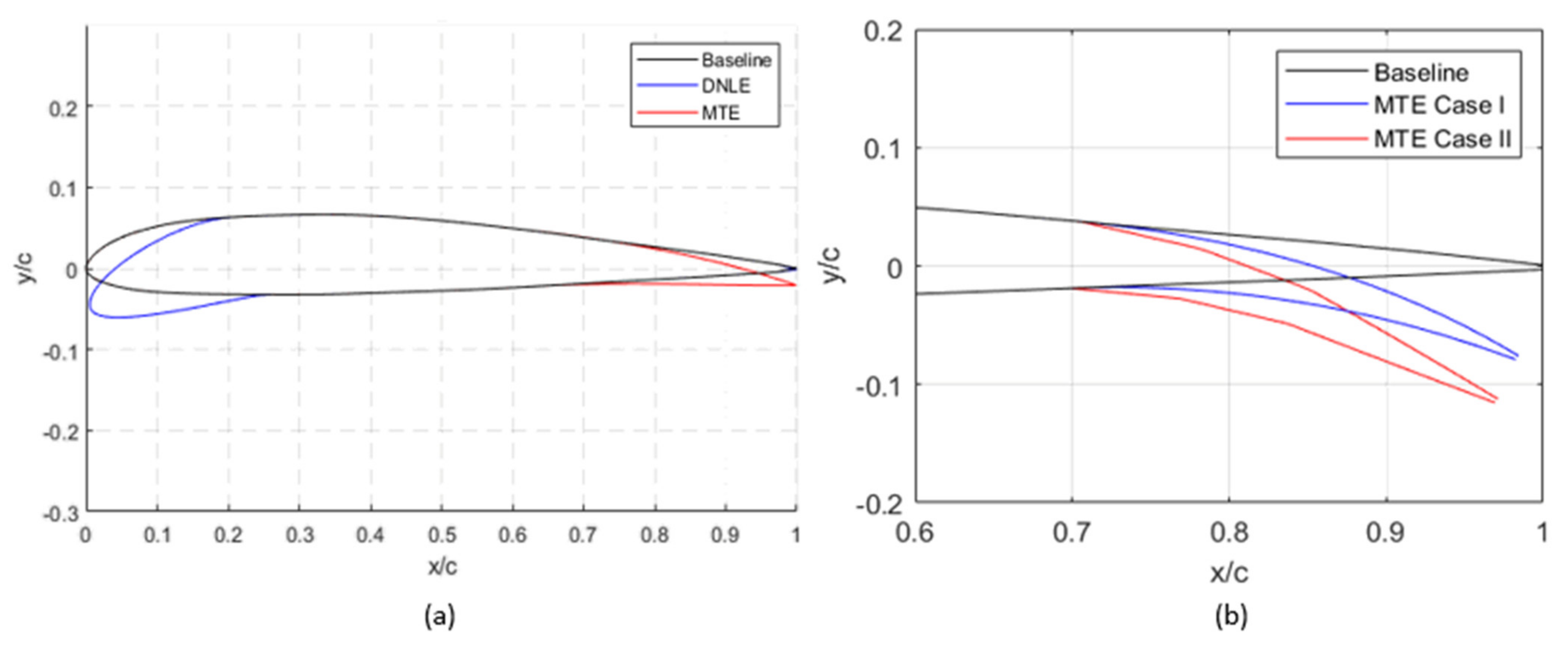
The aim of this study is thus to investigate the aerodynamic optimization by employing constrained shape parameterization for UAS-S45 root airfoil using Droop Nose Leading Edge (DNLE) and Morphing Trailing Edge (MTE) technologies. The aerodynamic design of continuous morphing wing surfaces employed to replace traditional discrete control surfaces, such as flaps, ailerons or sometimes slats, to adjust the camber of the wing, are discussed in this paper along with the parameterization strategy and the optimization algorithm.

1.2. Literature Survey

The potential in the field of aircraft morphing is evident as hundreds of research groups worldwide have been dedicated to studying the different aspects of morphing. Two of the earliest groups were launched by NASA, and they worked within the “Active Flexible Wing program” and the “Mission Adaptive Wing program” [18,19]. In these programs, flutter suppression, load alleviation and load control during rapid roll maneuvers were investigated.
One of the potential consequences of flexible morphing structures is that both dynamic properties and aerodynamic loads of the wing are affected. Hence, the aeroelastic effects arising from interactions between the configuration-varying aerodynamics and the morphing structure are significant. Li et al. have presented important morphing studies in terms of aeroelastic, control and optimization aspects [20].
The nonlinear aeroelastic behaviour of a composite wing with morphing trailing-edge has been studied [21]. Moreover, the nonlinear aeroelastic behaviour of a composite wing with morphing trailing-edge has been studied.
Aero-elastically stable configurations of a morphing wing trailing edge driven by electromechanical actuators have been investigated [22]. The effects induced by trailing-edge actuators stiffnesses on the aeroelastic behaviour of the wing were simulated using different approaches. The results revealed that flutter could be avoided if sufficient stiffness was provided by these actuators.
An analytical sensitivity calculation platform for flexible wings has been studied [23,24]. This platform has been used to perform wing aeroelastic optimization and stability analysis.
In another study, a low-fidelity model of an active camber aero-elastic morphing wing was developed to investigate the critical speed values by varying its chord-wise dimension [25]. A wide range of configurations was explored to predict the dynamic behaviour of these active camber morphing wings.
The combined flutter behaviour and gust response of a series of flexible airfoils has been investigated [26]. Rayleigh’s beam equation was used to model this series of flexible airfoils. The effect of chordwise flexibility of a compliant airfoil was investigated numerically to demonstrate its dynamical stability [27,28]. An actuated two-dimensional membrane airfoil was investigated experimentally and numerically, and it was found that membrane flexibility decreased the drag and delayed the stall.
These aeroelastic studies are significant in understanding the flexible morphing wing and its potentially relevant effects. However, our study does not consider the structural effects of morphing, and therefore the optimization is aimed to improve the aerodynamic drag performance and endurance in the given range of angles of attack.
Other research projects in the US and Canada include the “Smart Materials and Structures Demonstration” program initiated to develop new affordable smart materials to establish the performance gains by investigating smart rotors, the smart aircraft and the marine propulsion system; the “Aircraft Morphing” program [29]; the “Advanced Fighter Technology Integration” (AFTI) program, aimed to develop and demonstrate in flight a smooth variable camber wing and flight control system capable of adjusting the wing’s shape in response to flight conditions to maximize aerodynamic efficiency; the “Active Aeroelastic Wing” program, demonstrated to improve aircraft roll control through aerodynamically induced wing twist on a full-scale high-performance aircraft at transonic and supersonic speeds; the “Morphing Aircraft Structures” program [30]; the “Mission Optimized Smart Structures” (MOSS), in which aerodynamic optimization was performed with the stretching of the leading edge using a novel skin material developed with a nanocomposite at the National Research Council of Canada [31]; and the “Controller Design and Validation for Laminar Flow Improvement on a Morphing Research Wing–Validation of Numerical Studies with Wind Tunnel Tests—CRIAQ MDO 7.1” [32,33]. The CRIAQ 7.1 project took place at our Laboratory of Applied Research in Active Controls, Avionics and AeroServoElasticity LARCASE.
The European Union has conducted several projects, including the “Active Aeroelastic Aircraft Structures” (3AS) project, to develop novel active aeroelastic control strategies to improve aircraft performance (structural weight, better control effectiveness) by controlling structural deformations to modulate the desired aerodynamic deformations [34]; the “Aircraft Wing Advanced Technology Operations” (AWIATOR) project, in which novel fixed wing configurations were introduced aimed at reducing the vortex hazard by implementing larger winglets and further improving aircraft efficiency and reducing farfield impact [35]; the “New Aircraft Concepts Research” (NACRE) project, in which Powered Tails and Advanced Wings were studied to obtain high environmental performance (noise and CO2 emissions)—both high aspect ratio low-sweep wings and forward-swept wings (with natural laminar flow) contributed to achieving good fuel efficiency [36]; the “Smart Leading Edge Device” (SmartLED) project [13]; the “Smart High Lift Devices for Next Generation Wings” (SADE) project [37]. Both SmartLED and SADE were aimed to develop and investigate the morphing high lift devices, “smart leading edge” to enable seamless high lift devices and therefore enable laminar wings and “smart single-slotted flap”, for the next generation aircraft of high surface quality for drag reduction. Projects by the European Union also included the “Smart Fixed Wing Aircraft” (SFWA) project [38] and the “Smart Intelligent Aircraft Structures” (SARISTU) project to address the physical integration of smart intelligent structural concepts. The SARISTU included a series of research collaborations to addresses aircraft weight and operational cost reductions as well as an improvement in the flight profile specific aerodynamic performance [39]. Other projects by the European Union were the “Novel Air Vehicle Configurations” (NOVEMOR) project, in which morphing wing solutions (span and camber strategies and wing-tip devices) were proposed to enhance lift capabilities and maneuvering [40]; the “Clean-Sky 1 and 2” projects [41,42]; the “Combined Morphing Assessment Software Using Flight Envelope Data” (CHANGE) project, which developed a modular software architecture capable of determining and achieving optimum wing shape [43]; and the “Sustainable and Energy Efficient Aviation” (SE2A) project aimed to investigate the Morphing structures for the 1g-wing to exploit the nonlinear structural behavior of wing design components to achieve passive load alleviation [44].
The “Morphing Architectures and Related Technologies for Wing Efficiency Improvement-CRIAQ MDO 505” was also realized at the LARCASE in the continuation of the CRIAQ 7.1 project mentioned above. The achievements of the international Canadian-Italian CRIAQ MODO 505 project are mentioned in various publications [45,46].
The aircraft optimization process has evolved dramatically over the past decades. The design of new intelligent algorithms and computational solvers has substantially impacted the overall design process, including the “morphing aircraft optimization”. The verification and validation of aircraft design using optimization techniques has reduced its huge experimental costs and has been achieved by the use of efficient algorithms and computational solvers [47,48]. An optimization process is initiated by minimizing or maximizing an objective function for the target design concept with respect to design variables subjected to given constraints, which were applied to limit the search space and therefore to yield physically feasible optimization results. Both gradient-based and gradient-free intelligent algorithms have been used in these optimization processes, and their results are dependent on the type of optimization problem to be solved [47]. These algorithms are discussed in the following sections. Many optimization techniques based on bioinspired processes and Surrogate-Assisted natural methods have been formulated, and mathematical and statistical analysis of these algorithms has been performed [49,50,51,
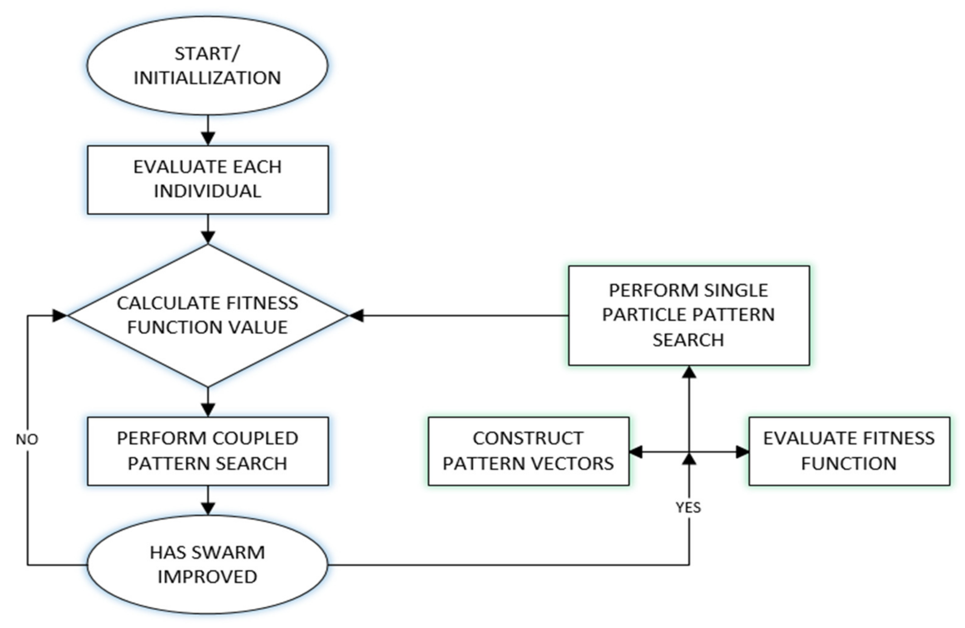
52]. The comparative performance study based on convergence trends was performed with different geometry parameterization techniques. Both advantages and disadvantages can be found in these optimization algorithms for complex shape functions. However, the goal of this study is to perform aerodynamic design optimization of morphing airfoil using Particle Swarm Optimization (PSO) algorithm combined with Pattern Search technique.
Similarly, various computational solvers are employed based on their desired solution accuracy and computational cost [53]. Researchers have conducted various aerodynamic and structural optimization studies, including design studies of different surfaces (components) of the wing, such as its upper surface, trailing edge or leading edge. Adjoint-based airfoil optimization has been studied using Euler equations [54], while other researchers have implemented extensive gradient-based aerodynamic shape optimization methodologies for transonic wing design using high-fidelity RANS solvers [55]. Many other optimization studies have been performed using different optimization techniques. Some of the most notable works are summarized in Table 1.
The study presented in this paper analyses the aerodynamic optimization of the Hydra Technologies S45 Balaam UAS airfoil. This unmanned aerial surveillance (UAS) system is needed to provide security and surveillance capabilities for the Mexican Air Forces, as well as civilian protection in dangerous situations. This study of Morphing Wing Technology has the aim to enhance the aerodynamic efficiency and the effective range of the UAS S45, as well as to extend the flight time. The next section of this paper presents the optimization framework of the overall methodology, which includes two objective functions’ formulations (“drag minimization” and “endurance maximization”). The parameterization technique is also presented in Section 2 and has the aim to obtain the “optimal aerodynamic shapes”; the computational solvers for calculating aerodynamic coefficients and the optimization algorithms employed are also presented. The results obtained by these solvers and algorithms for the UAS-S45 optimized designs are compared with the baseline UAS-S45 model results.

2. Method

This optimization framework study performs the aerodynamic optimization of the leading edge and trailing edge of a morphing airfoil by using an intelligent and iterative process based on user-defined aerodynamics and constraints. The methodology involves the objective function formulation integrated with a geometrical shape parameterization model, an aerodynamic flow solver and the optimization algorithm.
For this study, an optimization framework is designed to allow the integration of shape generation using the direct manipulation of the airfoil shape variables while respecting the geometrical constraints. The optimization procedure framework is described in Figure 2, and it consists of a parameterization block based on the Bezier–Parsec (BP) parameterization airfoil shape technique and an aerodynamic solver, such as the panel solver XFOIL (Version 6.99, MIT, USA, 2013 ). The validation of its results is done using high-fidelity solver in Fluent based on Reynolds-averaged Navier–Stokes (RANS) equations in the Transition SST model. A hybrid optimizer based on Particle Swarm Optimization (PSO) algorithm combined with the Pattern Search technique is also used. The optimization procedure is shown in Figure 2 and is described in detail in Section 2.1, Section 2.2, Section 2.3, Section 2.4.

2.1. Objective Function Definition

Numerous researchers have stated that there is always a trade-off between aerodynamic coefficients and performance parameters in aerodynamic design problems [66]. A difficult balance exists between increasing aircraft performance and meeting design constraints efficiently in practical aerodynamic design problems. For example, the objective of aerodynamic optimization is lift maximization, drag minimization or maximization of the lift-to-drag ratio while keeping CL and/or CD constant as constraints. Likewise, various airfoil shapes are optimized for their morphing by considering an increased lift-to-drag ratio and, at the same time, for meeting the given constraints. Other airfoil shape optimizations may involve those of multiple aerodynamic coefficients based on performance parameters such as range, loiter and control. Such optimization techniques can be applied to solve complex aerodynamic design problems for a broad range of flight conditions.
In addition, the design problem shown in this paper must consider the extended range of flight operating conditions that a UAV is expected to encounter within its flight envelope. As mentioned above, this study considers the optimization of the airfoil shape for drag minimization and for endurance maximization as individual target objective functions.
The mathematical formulation of the drag minimization objective function is the following.
m i n i m i z e   C D x ; x   ϵ   a i r f o i l   s e t
Su bject   to
C L m a x   ( x ,   α ,   M   ) 1 · 608 C L m o r p h C L m i n ,   b a s e l i n e x ,   α ,   M
where
  x a i r f o i l   s e t , t h e   v e c t o r   o f   a i r f o i l   s h a p e   f u n c t i o n   d e s i g n   v a r i a b l e s  
The lift coefficients of the UAS-S45 are calculated for each angle of attack using design parameters mentioned in a previous paper of our team [67]. The constraints implemented are both maximum lift coefficient and lift coefficient of baseline airfoil at each angle of attack. The optimization runs are executed with a minimum lift coefficient at each angle of attack. Constraints are applied by penalty functions to the objective function to ensure optimum performance is obtained at each given angle of attack.
For the design of a long-endurance UAV, Equations (2) and (3), which are needed to determine the endurance (E) of a propeller-powered UAV, are well established using the Breguet formula [68].
E = η p r c p C L 3 2 C D 2 ρ S   1 W f 1 W i
where c p is the specific fuel consumption, η p r is the propeller efficiency, ρ is the free stream density, S is the wing planform area, W i is the initial weight of the aircraft, W f is the final weight of the aircraft and C L and C D are the lift and drag coefficients, respectively.
The parameters that do not affect the airfoil shape design in the endurance performance can be neglected in Equation (2), and the parameters that can affect the airfoil shape design are only the two aerodynamic coefficients C L and C D ; therefore, Equation (2) can be reformulated as
E a = C L 3 2 C D
Therefore, an optimized airfoil maximizes the lift and minimizes the drag coefficients in the above Equation (3); therefore, the overall endurance aerodynamic efficiency is maximized. The weighted average of the flight envelope is used to find out the time that the UAV would have to spend in different flight regimes. Since the present study concerns the surveillance UAS-S45 optimization, it is assumed that 80% of total flight time is spent in loiter flight conditions, which require maximum endurance. Therefore, the objective function to maximize the endurance aerodynamic efficiency with the same constrained optimization is given by the following equation:
maximize   E a x = C L 3 2 C D
where x a i r f o i l   s e t , t h e   v e c t o r   o f   a i r f o i l   s h a p e   f u n c t i o n   d e s i g n   v a r i a b l e s  

2.2. Parameterization Strategy

Parameterization of the airfoil shapes for the UAS design and optimization requires a mathematical formulation, and it becomes an important part of the overall optimization process. Studies have shown that the choice of shape parameterization technique has a strong influence on the solution accuracy, robustness and computational time of the overall optimization process [69]. In order to obtain an optimal aerodynamic solution, the shape function must be directly related to the airfoil geometry, have a flexible design space, and be robust for the control of all parameters. Some of the well-known methods are the Discrete Based Approach, the Bezier curves, the B-Spline or NURBS curves, the Cubic Spline and the Free-Form Representation [69,70]. The drawbacks of these methods are that they do not use airfoil shape parameters, they require a large number of design variables and they often provide inaccurate shapes for the leading edge and trailing edge of an airfoil.
These limitations have been partly removed by using the polynomial-based functions, such as PARSEC and CST. “PARSEC” is characterized by eleven design coefficients that control airfoil shape parameters, and they are the: (a) edge radius, (b) upper crest abscissa, (c) upper crest ordinate, (d) upper crest curvature, (e) lower crest abscissa, (f) lower crest ordinate, (g) lower crest curvature, (h) trailing edge ordinate, (i) trailing edge thickness, (j) trailing edge direction and (k) trailing edge wedge angle. Several studies have shown PARSEC method’s superior performance with respect to the Discrete Based Approach, based on their convergence rate, flexibility and epistasis, which is due to the nonlinear dependency of the objective function on the design parameters [71]. However, it has also been found that the leading edge and trailing edge design coefficients in this parameterization method do not provide accurate airfoil shape; therefore, implementing morphing design using only these PARSEC design coefficients might further increase the airfoil shape complexity.
Therefore, a combined approach, the Bezier-PARSEC (BP) parameterization method, was developed [72] that included the advantages of Bezier with PARSEC combination, and it was found to be suitable for this study. The BP parameterization was implemented in this paper with the aim to increase the solution accuracy, flexibility and efficiency of morphing leading edge and trailing edge optimizations. More significantly, this technique provides the large search space needed for morphing leading edge and trailing edge design, and it reduces the computational time.
The BP method has been further divided into two parameterization sub-methods: BP3333 and BP3434. Four third-order Bezier curves are used to represent the airfoil shape in the BP3333 parameterization sub-method. The BP3434 parameterization has a 3rd-degree edge thickness curve, a 4th-degree trailing edge thickness curve, a 3rd-degree leading edge camber curve and a 4th-degree trailing edge camber curve. Due to the smaller number of degrees of freedom in the BP3333 method with respect to those of the BP3434 method, specifically at the trailing edge and at the leading edge, the BP3434 method was chosen in this research.
A fourth-degree Bezier curve is given by:
x u = x 0 1 u 2 + 4 x 1 u 1 u 3 + 6 x 2 u 2 1 u 2 + 4 x 3 u 3 1 u + x 4 u 4
and
y u = y 0 1 u 2 + 4 y 1 u 1 u 3 + 6 y 2 u 2 1 u 2 + 4 y 3 u 3 1 u + y 4 u 4
The parameterization is controlled by 15 parameters: 10 aerodynamic and 5 Bezier parameters. Figure 3 shows the graphical representations of these parameters.
The control points definitions for the leading and trailing edge Bezier curves are given in Table 2 for the thickness profile curve, and in Table 3 for the camber profile curve [73]. The upper and lower bound values of the parameters used in the BP parameterization optimization method calculated in this study for the UAS-S45 are presented in Table 4.

2.3. Description of Flow Solvers

Various solvers have been employed in aerodynamic optimization studies, such as the Fully Potential Flow, Coupled Boundary-Layer, Euler and Viscous Navier–Stokes solvers [74]. The type of solver chosen by a user depends upon the type of optimization problem. Results obtained with the flow solver must be consistently accurate in order for the optimization to be considered highly adequate.
For this aerodynamic research, incompressible flow solvers are needed as they can perform fast computation, and also can provide high accuracy results. Therefore, in this paper, two types of aerodynamic solvers are used for the aerodynamic optimization: a Panel-based method and a Reynolds-Averaged Navier–Stokes equations (RANS) solver. The choice to keep the computational cost low for an airfoil analysis leads directly to the use of the XFOIL code, which is known for its very good combination of execution speed and accuracy of results. Furthermore, in order to obtain higher accuracy results for solving the viscous boundary layer and the flow separation than the XFoil solver, a well-established high-fidelity Computational Fluid Dynamics (CFD) solver, Ansys Fluent was also used in this morphing airfoil analysis.

2.3.1. XFoil

XFoil is a code for airfoil design and analysis consisting of inviscid, inverse and viscous formulations [75]. The viscous formulation can be used to calculate free or imposed forced flow transition to handle transitional separation bubbles, to calculate aerodynamic coefficients and to cope with moderately trailing edge separation. It uses an approximate eN envelope method to calculate the flow transition. The turbulence level settings are kept as default with free transition features. Both the boundary layer and the wake parameters are calculated with a two-equation integral boundary layer formulation as shown in Equations (8) and (9), respectively [76].
d θ d ξ + 2 + H M e 2 θ u e d u e d ξ = C f 2 + υ 0 u e
θ d H * d ξ + 2 H * * + H * 1 H θ u e d u e d ξ = 2 C D H * C f 2 + 1 H * υ 0 u e
where shape factors H * and H * * are defined in the following equations
x H * = 0 u U 1 u U 2 d y 0 u U 1 u U d y
and
H * * = 0.064 H k 0.8 + 0.251 M e 2   with   H k = H 0.290 M e 2 1 + 0.113 M e 2
At high angles of attack where stall occurs, XFoil has difficulties in giving a converging solution for the airfoil analysis. To obtain the convergence of the solution, non-converged solutions are given a high penalty by setting the fitness function arbitrarily large via a penalty function, and thus they are eventually eliminated during the design process. The solver tolerance value used for this penalty function calculation is 0.002.
Many researchers have employed XFoil software in morphing airfoil studies. In one of these studies, the results obtained using XFoil were compared with those obtained using the Reynolds-Averaged Navier–Stokes (RANS) solvers for camber morphing, and only a slight difference between the results was observed [77].

2.3.2. CFD Fluent Solver

The validation of solvers and mesh settings is needed before carrying out the optimization studies. The validation studies were performed at a Reynolds number of 2.4 × 10⁶ and a Mach number of 0.10. The range of angles of attack was considered from 0° to 16° to include the stall angle. The aerodynamic coefficients and the pressure distribution were obtained and further used for solution validation. A C-shaped computational domain with structured grids, as seen in Figure 4, was used in domain discretization after the performance of the mesh convergence test. The turbulence model used in this study was the Transition γ R e θ SST. This model uses a combination of SST K-ω coupled with intermittency γ and transition onset Reynolds number. R e θ is the critical Reynolds number where the intermittency starts [78]. Four transport equations of the Transition γ R e θ SST model are given below:
ρ k t + ρ U j k x j = P k D k + x j μ + σ k μ t k x j
ρ ω t + ρ U j ω x j = P ω D ω + x j μ + σ ω μ t ω x j + 2 1 F 1 ρ σ ω 2 ω k x j ω x j
ρ γ t + ρ U j γ x j = P γ E γ + x j μ + μ t σ γ γ x j
ρ R e θ t ¯ t + ρ U j R e θ t ¯ x j = P θ t + x j σ θ t μ + μ t R e θ t ¯ x j
The spatial discretization used in the solution is of the second order for all the turbulence statistical parameters, including the momentum, the turbulent kinetic energy, the specific dissipation rate, the intermittency and the Reynolds momentum thickness.
ANSYS Fluent was used in this study to carry out the numerical analysis. The meshing was done using ANSYS Mesher, as shown in Figure 4. The rectangular computational domain was designed around the airfoil geometries. The outlet length was selected to be 30c, which was adequate to allow for the full development of the wake flow, based on the size of the computational domain adopted in previous studies. The distance from the domain inlet to the airfoil was 10c to prevent the inlet boundary from unphysically impacting the induction field upstream of the airfoil. The high-quality grids were generated with dense grids in the boundary layer of the airfoil with a gradual decrease of grid cells away from the airfoil surface. The first layer’s thickness was calculated based on inlet velocity and adopted accordingly to capture the laminar and transitional boundary layer regions. Furthermore, the grid sensitivity analysis was performed according to the number of cells in the computational domain.
A freestream velocity of 34 m/s with a turbulence rate of 0.01 percent was imposed at the inlet. The surface of the airfoil was modelled as a zero-roughness no-slip wall, and its values were executed on the grid domain, which prescribed its motion relative to the rest of the computational domain. A symmetry boundary condition was applied to achieve a parallel flow at the top and bottom of the domain by assuming zero normal velocity and zero normal gradients of the flow quantities. A zero static gauge pressure was applied at the exit of the domain. Iterations were finalized when all scaled residuals were below 1 × 10⁶.

2.4. Optimization Algorithm

An intelligent search algorithm is essential for the direct numerical optimization of airfoil design. This algorithm operates iteratively and utilizes the inputs of the shape parameterization method to define the airfoil shape, and then it uses the flow solver to calculate the aerodynamic coefficients. Its efficiency is assessed according to its ability to provide a global optimal solution with reasonable computational resources. Therefore, the choice of such an algorithm influences the solution convergence and its feasibility.
Researchers have implemented various algorithms, such as the Gradient-Based, Adjoint-Based and Evolutionary algorithms with the aim to investigate and solve various optimization problems [74]. These algorithms have been considered to solve different aerodynamic optimization problems based on their advantages and disadvantages. The hybrid optimizer based on the Particle Swarm Optimization (PSO) algorithm was used in this paper for the UAS-S45 optimization, and it was further combined with the Pattern Search algorithm in order to enhance the solution convergence and its refinement.
Evolutionary algorithms have attracted the attention of shape designers due to their characteristics, such as their suitability for modelling discontinuous shape functions, obtaining global optimal solutions, ease of parallel computing, etc. During morphing airfoil optimization, gradient-based algorithms converge fast, but they only cover a small area out of a large airfoil search space, and thus a local minimum solution instead of global minimum solution is found. It is also difficult to find the gradient of the non-linear flow fields for gradient-based optimizers.
Therefore, a PSO algorithm is used, based on a simplified social behavior closely related to the swarming theory, where the solutions are represented by a set of particles that heuristically navigate through a design space [79]. The efficiency of PSO algorithms over genetic algorithms is due to their independence from parameters, such as crossovers and mutations; instead, the solution is updated by sharing its information amongst its populations of particles.

2.4.1. PSO Algorithm

In the PSO algorithm, each particle is a solution to a given optimization problem and is composed of two vectors: “position” and “velocity”. A position vector   x i n is used to store the positioning of the particles in the given dimensional space. The velocity vector v i n is updated using the following equation for each iteration k:
v i n   k = v i n k 1 + c 1 r 1 p b e s t i n x i n k 1 + c 2 r 2 p b e s t g i n x i n k 1
where x i n   = position vector; v i n = randomly generated velocity vector of the particles at search initialization; p b e s t i n = vector representing the best solution achieved by the particle; p b e s t g i n = vector representing the “global best solution” collectively achieved by the swarm; c 1 and c 2 = stochastic acceleration terms that pull each particle toward p b e s t i n and p b e s t g positions respectively; r 1 and r 2 = random numbers in the uniform range [0, 1];
The update of the position vector at the k t h iteration is given by the following equation:
x i n k = x i n k 1 + v i n k
The PSO procedure can be outlined as follows:
  • Generate an initial swarm with arbitrary values of the particle position and arbitrary initial velocities in the n-dimensional search space;
  • Evaluate the fitness of each particle of the swarm by searching a new velocity vector applied to each individual particle; the new velocity vector is influenced by its best position, the swarm’s best position and its previous velocity;
  • Update the velocity of the particles as shown in Equation (14) and the position of the particles as shown in Equation (15) and evaluate the new fitness function;
  • Repeat steps 2 and 3 until the maximum number of iterations is reached or until the results no longer improve for a given number of iterations.
Pattern Search (PS) is a direct search optimization method that is used to minimize a function by comparing its value at each iteration with its value at its previous iteration in a finite set of trial points. The method is outlined as follows:
  • Select the initial solution;
  • Explore the direction search by evaluating each objective function value, one at a time;
  • Evaluate the objective function. If the objective function is minimized, then update it; otherwise, do not update it;
  • Evaluate the next values of the objective function following the previous steps 2 to 3;
  • After exploring the search of all possible values of the objective function and the minimization of the overall objective function, the PS method follows a pattern move; and
  • If the overall objective function has not been minimized, repeat the process.

2.4.2. Hybrid Optimization Scheme

A hybrid optimizer is used in this study, as shown in Figure 5. In this figure, the hybrid optimization implies that the PSO-based optimization process is applied firstly to its variables to obtain their optimized values. Since the first optimization process may not be accurate as it would result in low variations of values to be optimized, a second optimization process would then be applied to the results of the first optimization process. In this case, PSO, a non-elitist algorithm, is then followed by Pattern Search, using hybrid optimization. The PSO and Pattern Search can then be used to find a local optimum in a limited search area; the use of both PSO and PS algorithms through hybrid optimization ensures better results than a single optimization process. The independent variables given as inputs to the optimization process are also limited due to their upper and lower bounds. These bounds ensure that the search space for both the PSO and Pattern Search algorithms remains within them. During the PSO algorithm execution, if a solution is found outside the bounds of the search space, any such solution outside these bounds will have its value replaced by that of its given upper and/or lower bounds, without any influence on other solutions. The hybrid optimizer’s procedure is shown in Figure 5.

3. Discussion and Results

The aerodynamic optimization considered in this study applies to both Droop Nose Leading Edge Morphing (DNLE) and Morphing Trailing Edge (MTE) configurations. To utilize the full potential of the “morphing” concept, a baseline shape optimization was carried out followed by its morphing shape design at various flight conditions given in Table 5. These cases are based on various altitudes and Reynolds numbers that are computed for the airspeed of 34 m/s. These given flight conditions are chosen because of the fact that the UAS-S45 can reach altitudes of 20,000 ft and a stall speed of 34 m/s. The design framework uses endurance maximization as an optimization function to enhance the performance of the UAS-S45 over a large part of its flight regimes. Figure 6 shows the flight envelope of UAS-S45. From a physical standpoint, every flight condition is defined by a specific Mach number, altitude (Reynolds number and temperature are calculated according to ISO standard atmosphere) and a fixed lift coefficient. The present study considered the optimization of the leading edge and trailing edge of the UAS S45 conventional wing that could be both morphed. The difference of performances obtained between the baseline airfoil and the morphed one demonstrate the overall benefits of morphing airfoil design. Figure 7 shows the design of Droop Nose Leading Edge (DNLE) and Morphing Trailing Edge (MTE) airfoil configurations versus the baseline airfoil. Figure 7a shows the basic concept of the morphing wing with combined morphing leading and trailing edge deflections and Figure 7b shows two cases of MTE designs.
Figure 8 shows the aerodynamic coefficients CL and CD variations of the baseline UAS-S45 root airfoil for two Reynolds numbers Re = 1.2 × 10⁶ and Re = 2.4 × 10⁶, which were calculated using the XFoil and the Transition γ R e θ SST in Ansys/Fluent software. As seen in Figure 8, the lift coefficients’ variations with the angle of attack were predicted accurately, while small differences were found in drag coefficient variations with the angle of attack. These differences in the drag coefficients’ variations are found largely at angles of attack higher than 4° because the pressure-based drag coefficient becomes the dominant component of the total drag coefficient and flow separation conditions result in a decreased friction-based drag coefficient. This result implies that drag forces are very sensitive to turbulence effects and the Transition γ R e θ SST model can solve the turbulence problems more accurately than the XFoil solver.
Figure 9a shows the friction coefficient variations with the chord for the angles of attack of 0°, 2° and 6° obtained by use of the Transition   γ R e θ SST model; this figure indicates very good accuracy in predicting the flow separation phenomena as the skin friction coefficient increases slightly with the increase in angle of attack. Figure 9a,b also shows the initial flow separation, the separated region and its reattachment. It is seen in Figure 9a that the laminar-to-turbulent transition region is located at 18% of the chord (0.18c) at an angle of attack of 6° and at 43% of the chord (0.43c) at an angle of attack of 2°.The variations of the skin friction coefficient along the chord were assessed at different angles of attack using the Transition γ R e θ SST model in Figure 9.
The velocity magnitude contours plots at three angles of attack (4°, 10°, 16°) at Re = 2.4 × 10⁶ are shown in Figure 10. The turbulent intensities play an important role in understanding the flow behavior over an airfoil, and they are shown in Figure 10 for the angles of attack of 4° and 10°.
The contour lines remain attached to the airfoil at low angles of attack such as 4°, as shown in Figure 10a; the flow starts to separate at the trailing edge of the airfoil at an angle of attack of 10° as shown in Figure 10b and changes into a fully separated flow at the angle of attack of 16° as shown in Figure 10c. It is important to understand that boundary layer separation takes place at an angle of attack of approximately 10°. The separation region shown in Figure 10c causes increased drag as it induces a large wake that completely changes the flow downstream of the point of separation. It is clear that the turbulent intensity is minimal at the airfoil leading edge at a low angle of attack of 4°, as seen in Figure 11a, while at the angle of attack of 10°, the turbulent intensity increases over the airfoil surface, including at its leading edge.

3.1. Optimization of Morphing Leading Edge

The Droop Nose Leading Edge (DNLE) optimization was performed to satisfy the objective functions defined in Equation (1) for drag minimization and in Equation (5) for endurance maximization. The optimization processes were carried out for two cases of DNLE control point deflections, defined as “Opt. Case I” and “Opt. Case II”.
In “Opt. Case I”, a morphing DNLE is a smooth single structural layout with a morphing leading edge starting location fixed at 22% of the chord. The trailing-edge is not allowed to move, while the leading edge points are only allowed to move in the vertical direction to effectively adapt the chord-length variation of the baseline airfoil.
In “Opt. Case II”, the morphing DNLE is free to change its shape anywhere from 0 to 22% of the chord. The starting point and the end point of the leading edge are used to represent the morphing DNLE shape. The parameterization of the DNLE shape was obtained by using the Bezier–PARSEC (BP) method, in which the leading edge radius of the airfoil and 5 Bezier control points were used to maintain the slope continuity within the airfoil shape.
The XFoil software was used to efficiently investigate the aerodynamics of the optimized morphing geometries. The aerodynamic performance of the DNLE was evaluated to determine its best airfoil design shape for each flight condition. The computations were performed for the three flight conditions listed in Table 5. The results were obtained in terms of aerodynamic lift and drag coefficients variations with angle of attack and pressure distributions versus the airfoil chord locations for the optimized airfoil geometries.
Figure 12a illustrates the initial (reference) versus the final (optimized or morphed) airfoil shape, while Figure 12b shows the convergence trend for the minimum drag optimization function for an optimized airfoil shape with DNLE at an angle of attack of 50. The algorithms PSO with Pattern Search converge to the optimal solution after 90 iterations. The x-axis indicates the number of function evaluations, and the y-axis shows the value of the fitness. The fitness value is the objective function value of each particle of the algorithm, expressing the performance of any airfoil shapes.
These results for the droop nose leading edge (DNLE) optimization are shown in Figure 13 and Figure 14, and the UAS-S45 baseline airfoil aerodynamic coefficients were compared to those of the optimized airfoils. Figure 13a–d show the variations of lift coefficients with the angles of attack. The lift coefficient variations for all three flight conditions for Opt. Case I and Opt. Case II and the baseline airfoil in Figure 13a–c show that higher lift coefficients were obtained for Opt. Cases I and II than those of the baseline airfoil. Figure 13d shows that the DNLE designs for Opt. Case I at three different flight conditions. It is found that Opt. Case I DNLE design is the best at Flight Condition III. These optimal shapes revealed that maximum increment of the lift coefficient with respect to the baseline airfoil of up to almost 21% was found for Opt. Case I design seen in Figure 13c. In addition, an increase of 9.6% was obtained for the maximum lift coefficient, associated with a stall angle delay of 3° as seen in Figure 13c. Therefore, it was found that both Opt. Case I and Opt. Case II results are better than the baseline airfoil results. These better results can be explained by the pressure distribution change around the airfoil. The DNLE design does not cause an adverse pressure gradient as the flap configuration, but instead, it decreases the maximum speed at the airfoil leading edge, which is similar to the findings [80].
Figure 14 presents the evaluation of the lift vs. drag polar of the baseline airfoil and of the optimized airfoils for three different flight conditions. Therefore, the increased aerodynamic performance of optimized airfoils in terms of their lift versus drag variation for all three flight conditions can be seen in Figure 14a–d.
The pressure coefficients’ variations with the chord of optimized airfoils for three flight conditions are shown in Figure 15. It is clear that the major changes in pressures take place near the leading edge at its upper surface, and that the pressure peaks then remain smooth on the rest of the airfoil for all configurations in Figure 15a for an angle of attack of 4° and in Figure 15b for an angle of attack of 10°. The chord-wise pressure distribution reveals that increased performance was obtained for DNLE configurations. By comparing the chord-wise pressure distributions for different configurations at angles of attack of 10° for the baseline versus optimized airfoils, it is found that a kink in the suction peak is followed by a constant pressure distribution. The DNLE-optimized configuration at flight condition III undergoes flow separation, and reattaches shortly on the airfoil surface, as seen in Figure 15b.
Figure 16a illustrates the initial (reference) versus the final (optimized or morphed) airfoil shape, while Figure 16b presents the convergence for aerodynamic endurance optimization while utilizing the PSO algorithm with Pattern Search for the DNLE-optimized airfoil at an angle of attack of 50°. A downward trend followed by constant values is clearly visible for the function, thus indicating the approach to the global optimum.
Figure 17 shows that the optimization process led to an increase in endurance maximization characterized by CL3/2/CD in the optimized DNLE airfoils for three different flight conditions. The maximum endurance capability given by CL3/2/CD for the same lift coefficient of the baseline airfoil to the lift coefficient of the morphing DNLE configuration Opt. Case I was found to be 1.17 and 1.21, respectively. Furthermore, the values of CL3/2/CD increased from 117 to 132, thus indicating better endurance performance for the UAS-S45 DNLE airfoil configurations than for its baseline airfoil at three flight conditions.
The flow transition behavior can be seen in the velocity contour plots of one of the DNLE airfoils, as shown in Figure 18a for an angle of attack of 4° and in Figure 18b for an angle of attack of 10°. The comparison of baseline airfoil and DNLE configurations at a 10° angle of attack shows that higher gradients are formed for the DNLE airfoil in comparison with those of the baseline airfoil, illustrated in Figure 10. However, the trailing edge flow separation region remains the same for both airfoils. In addition, the Turbulent Kinetic Energy (TKE) for the baseline airfoil and for the DNLE airfoils by use of the Transition γ R e θ SST turbulence model are shown in Figure 18c,d. It is evident that the leading edge is propagating the energy towards the downstream; thus a considerable decrease is observed in the wake turbulence. The TKE occurring in the baseline airfoil, which starts from the upper surface and moves towards the trailing edge was not observed in the DNLE-optimized airfoil at an angle of attack of 4°, as seen in Figure 18c.

3.2. Morphing Trailing Edge Optimization

The optimization process defined in Section 3.1 was implemented on the MTE airfoil by using the same two optimization functions defined by Equation (1) for drag minimization and by Equation (5) for endurance maximization. The optimization of the Morphing Trailing Edge (MTE) airfoil shape for the three flight conditions given in Table 5 was performed.
The optimization processes were carried out for two types of MTE control points. In the first type, referred to as Opt. Case I, MTE is a smooth single shape with a morphing starting point and trailing edge end point. The leading edge is not allowed to move, while the trailing edge points are only allowed to move in the vertical direction with respect to the baseline airfoil.
In the Opt. Case II, the MTE is a three-segmented finger-like configuration. The points are outlined to represent the morphing trailing edge starting location, the length of the first segment and the length of the second segment. The morphing location was kept at x/c = 0.60, so that enough space was provided for the actuation mechanism, and which is where its upper and lower limits were given as constraints. The upper bounds and the lower bounds were chosen to prevent the generation of morphing airfoil shapes with no likelihood of having very good aerodynamic efficiency. XFoil was used as an aerodynamic solver and therefore as a powerful tool that allowed obtaining fast convergence solutions. The results were later validated by the use of a RANS models in Ansys/Fluent solver.
Figure 19a illustrates the initial (reference) versus the final (optimized or morphed) airfoil shape, while Figure 19b illustrates the convergence trend for the minimum drag optimization function for an optimized airfoil shape with MTE at an angle of attack of 50. It is seen that the graph in Figure 19b trends to a constant after some iteration steps, which shows convergence to its optimal solution.
The first set of results obtained for MTE for different flight conditions are shown in Figure 20a–d. The lift coefficients are presented for the three different flight conditions in the two different cases of Opt. Case I and Opt. Case II. The lift coefficients of the optimized airfoil design have higher values than those of the baseline airfoil; therefore, the optimized shapes produce an improvement of the lift coefficient with respect to the baseline airfoil of up to almost 26%, as seen in Figure 20c for Opt. Case I. In addition, an increase of 8% is obtained for the maximum lift coefficient for the optimized airfoils with respect to the baseline airfoil.
Figure 21 presents the evaluation of the lift versus drag variation (polar) of the baseline airfoil and the optimized airfoils for different flight conditions. The increased aerodynamic performance of optimized airfoils for all three flight conditions can be seen in Figure 21a–d.
The pressure coefficients of the MTE airfoil cases at three different flight conditions are shown in Figure 22. It can be observed that the suction peaks of the optimized airfoils are higher than those of the baseline airfoil. The MTE airfoil results expressed in terms of “effective camber change” lead to a significant increase in the negative pressure value at the trailing edge surface. The low performance of the baseline airfoil compared to that of the optimized airfoils can be related to the unfavorable pressure gradient on its upper surface near the leading edge, thereby causing an earlier laminar–turbulent transition of the boundary layer by slightly increasing the drag.
Figure 23a illustrates the initial (reference) versus the final (optimized or morphed) airfoil shape, while Figure 23b presents the convergence graph of the aerodynamic endurance optimization for the given MTE optimized airfoil while utilizing the PSO algorithm with pattern search. Figure 23b shows that the algorithm performs well and improves the airfoil shape to maximize the endurance.
The optimization process using the endurance maximization objective function led to improved endurance performance in the optimized airfoils with respect to the endurance performance of the baseline airfoil. The performance measured in terms of CL3/2/CD variation with CL is shown for three different flight conditions in Figure 24. The endurance performance of each optimized airfoil shows a higher value in the MTE Opt. Case I with respect to its baseline airfoil configurations. For the same endurance performance defined by the CL3/2/CD ratio, the lift coefficients were found to be 1.17 for the baseline airfoil and 1.45 for the MTE airfoil configuration for the optimized flight condition II, respectively. Furthermore, as seen in Figure 24, the efficiency of CL3/2/CD increased by approximately 10.25% for flight condition III; this finding indicates the improved endurance performance of the UAS-S45 airfoil.
The difference between the results obtained by the two objective functions of drag minimization and endurance maximization to obtain optimal airfoil configurations was determined. The optimized airfoil geometrical shapes were obtained for drag minimization and endurance maximization as shown in Figure 25. The main difference observed in the airfoil geometries, as shown in Figure 25, is that the trailing edge obtained with the drag minimization objective function gave a smaller deflection than the baseline airfoil. Likewise, the endurance maximization objective function requires higher airfoil deflection with a continuous trailing edge.
The contour plots of the velocity magnitude and of the turbulent kinetic energy are visualized for the baseline airfoil and for the airfoils optimized by the Transition γ R e θ SST turbulence model in Figure 26. These contour plots reveal that for a given MTE deflection, larger TE separation regions are found at 4° angles of attack than at 10° angles of attack. Similarly, the vertex of turbulent kinetic energy (TKE) originating from the MTE at an angle of attack of 40° has more strength than the vertex an the angle of attack of 10°. The TKE contour plot of the baseline airfoil at an angle of attack of 4° is approximately comparable to the TKE contour plot of the MTE airfoil at an angle of attack of 10°. Therefore, the MTE-optimized airfoils can provide increased aerodynamics performance with respect to the performance of the original airfoils.

4. Conclusions

This study was conducted to perform aerodynamic optimization of Morphing Trailing Edge (MTE) and Droop Nose Leading Edge (DNLE) airfoils for the UAS-S45 at different flight conditions. A new hybrid optimization technique was chosen by coupling the Particle Swarm Optimization (PSO) with the Pattern Search (PS) algorithms. The optimization function was designed to minimize drag with respect to given constraints such as airfoil lower and upper bounds, as well as to increase endurance in given flight conditions. The Bezier–PARSEC (BP) technique was used to parameterize the baseline airfoil shape, as well as to obtain its various optimized morphing configurations by using different constraints on the morphing of both the Morphing Trailing Edge (MTE) and the Droop Nose Leading Edge (DNLE) of the wing.
Within the aerodynamics optimization framework, the low-fidelity solver XFoil and the high-fidelity CFD solver Ansys Fluent were used. The results obtained using both solvers were compared for their validation. Specifically, the flow transition was predicted using Menter’s Transition γ R e θ SST turbulence model. In addition, the optimization framework was done from an aerodynamics perspective, and therefore, no structural studies were taken into consideration.
Both DNLE and MTE airfoil optimizations were aimed to increase the aerodynamic performance of the UAS-S45 for a wide range of angles of attack. For each of the three considered flight conditions, enhanced aerodynamic efficiency was obtained by optimizing the morphing airfoil design with respect to its UAS-S45 baseline airfoil. The optimization results have shown an increase of lift coefficients in DNLE airfoils until the stall angle of attack and thus a delay in the stall angle. An improvement in the lift coefficient was produced for the DNLE airfoils with respect to the baseline airfoil of up to 21%. In addition, an increase of 9.6% was obtained for the maximum lift coefficient, and the stall angle was also delayed by 3 degrees. Similarly, the aerodynamic performance showed a significant improvement for the MTE configurations. An increase in the maximum lift coefficient of up to 8.13% and of the efficiency of CL3/2/CD by 10.25% was obtained, thus indicating an increased endurance performance for the MTE airfoils of the UAS-S45. The delay of the leading edge separation by use of DNLE airfoils was another interesting result.
The flight conditions were chosen from the UAS-S45 manufacturer Hydra Technology user manual. These conditions do not cover aircraft maneuvers or gust responses. UAS-S45 maneuvers and gust response studies could be done in the future. Other objectives of this morphing optimization study will include the three-dimensional analysis of a UAS-S45 wing with a combined droop nose leading edge (DNLE) and continuous morphing trailing edge (MTE). The improvements at the performance level, such as the typical fuel savings with the optimized morphing concepts for a given flight mission, will also be studied in the future. Based on the aero-structural studies, various configurations will be analyzed, and the internal actuation mechanism will be implemented. Wind tunnel and flight tests could be further performed to validate the optimized UAS-S45 model.

Author Contributions

Conceptualization; methodology, M.B.; software, S.L.-M., and M.B.; validation, M.B.; investigation, M.B., and S.L.-M.; writing—original draft preparation, M.B.; writing— review and editing, R.M.B.; visualization, M.B., S.L.-M. and R.M.B.; supervision, R.M.B.; and T.W.; funding acquisition, R.M.B. All authors have read and agreed to the published version of the manuscript.

Funding

This research received no external funding.

Institutional Review Board Statement

Not applicable.

Informed Consent Statement

Not applicable.

Data Availability Statement

The data presented in this study are available on request from the corresponding author.

Acknowledgments

Special thanks are due to the Natural Sciences and Engineering Research Council of Canada (NSERC) for the Canada Research Chair Tier 1 in Aircraft Modelling and Simulation Technologies funding. We would also like to thank Odette Lacasse for her support at the ETS, as well as to Hydra Technologies’ team members Carlos Ruiz, Eduardo Yakin and Alvaro Gutierrez Prado in Mexico.

Conflicts of Interest

The authors declare no conflict of interest.

Nomenclature

c l Lift force per unit span
c d Drag force per unit span
C L Lift coefficient
C D Drag coefficient
c Chord
c p Specific fuel consumption
C f Skin friction coefficient
D Drag force
D k Destruction term (Turbulent kinetic energy)
D ω Destruction term (Specific Dissipation Rate)
d z t e Trailing edge thickness
e Non-dimensional Oswald efficiency number
E Endurance
  E a Aerodynamic Endurance Efficiency
E γ Source terms (Vortex)
f Function
H Shape factor
k Turbulent kinetic energy
L Lift force
M Mach number
P k Production term (kinetic energy)
r l e Leading edge radius
R e θ Reynolds number with respect to the momentum thickness
S Wing planform area
U Boundary layer edge velocity
v i n Velocity vector
V Free stream velocity
W i Initial weight of the aircraft
W f Final weight of the aircraft
  x i n Position vector
x c Upper crest position in horizontal coordinates
y c Upper crest position in vertical coordinates
z t e Trailing edge offset in the vertical direction

Greek Symbols

α Angle of attack
α t e Trailing edge direction
β t e Trailing edge wedge angle
η p r Propeller efficiency
ρ Free stream density
Differential operator
θ Momentum thickness
ξ Streamwise coordinate
μ Dynamic viscosity coefficient
σ Source
ω Specific Dissipation Rate
γ Vortex

References

  1. BBC News, Q. ATAG Beginner’s Guide to Aviation Efficiency; The Intergovernmental Panel on Climate Change (IPCC): Geneva, Switzerland, 2019. [Google Scholar]
  2. Gerhards, R.; Szodruch, J. Industrial Perspectives of Drag Reduction Technologies. In Aerodynamic Drag Reduction Technologies; Springer: Berlin/Heidelberg, Germany, 2001; pp. 259–266. [Google Scholar]
  3. Valasek, J. Morphing Aerospace Vehicles and Structures; John Wiley & Sons: Hoboken, NJ, USA, 2012; Volume 57. [Google Scholar]
  4. Botez, R. Morphing wing, UAV and aircraft multidisciplinary studies at the Laboratory of Applied Research in Active Controls, Avionics and AeroServoElasticity LARCASE. Aerosp. Lab 2018, 1–11. [Google Scholar] [CrossRef]
  5. Barbarino, S.; Bilgen, O.; Ajaj, R.M.; Friswell, M.I.; Inman, D.J. A review of morphing aircraft. J. Intell. Mater. Syst. Struct. 2011, 22, 823–877. [Google Scholar] [CrossRef]
  6. Ameduri, S.; Concilio, A. Morphing wings review: Aims, challenges, and current open issues of a technology. Proc. Inst. Mech. Eng. Part C J. Mech. Eng. Sci. 2020. [Google Scholar] [CrossRef]
  7. Communier, D.; Botez, R.M.; Wong, T. Design and Validation of a New Morphing Camber System by Testing in the Price—Païdoussis Subsonic Wind Tunnel. Aerospace 2020, 7, 23. [Google Scholar] [CrossRef] [Green Version]
  8. Botez, R.; Koreanschi, A.; Sugar-Gabor, O.; Mebarki, Y.; Mamou, M.; Tondji, Y.; Guezguez, M.; Tchatchueng Kammegne, J.; Grigorie, L.; Sandu, D. Numerical and experimental transition results evaluation for a morphing wing and aileron system. Aeronaut. J. 2018, 122, 747–784. [Google Scholar] [CrossRef]
  9. Ameduri, S.; Galasso, B.; Ciminello, M.; Concilio, A. Shape memory alloys compact actuators for aerodynamic surfaces twisting. In Proceedings of the AIAA Scitech 2020 Forum, Orlando, FL, USA, 6–10 January 2020; p. 1299. [Google Scholar]
  10. Marino, M.; Sabatini, R. Advanced lightweight aircraft design configurations for green operations. In Proceedings of the Practical Responses to Climate Change Conference, Melbourne, Australia, 27 November 2014; p. 207. [Google Scholar]
  11. Noviello, M.C.; Dimino, I.; Amoroso, F.; Pecora, R. Aeroelastic Assessments and Functional Hazard Analysis of a Regional Aircraft Equipped with Morphing Winglets. Aerospace 2019, 6, 104. [Google Scholar] [CrossRef] [Green Version]
  12. Dimino, I.; Pecora, R.; Arena, M. Aircraft morphing systems: Elasticity of selected components and modelling issues. In Proceedings of the Active and Passive Smart Structures and Integrated Systems XIV, 19 May 2020; p. 113760M. [Google Scholar]
  13. Pantelakis, S.; Horst, P.; Kintscher, M.; Wiedemann, M.; Monner, H.P.; Heintze, O.; Kühn, T. Design of a smart leading edge device for low speed wind tunnel tests in the European project SADE. Int. J. Struct. Integr. 2011, 2, 383–405. [Google Scholar]
  14. Carossa, G.M.; Ricci, S.; De Gaspari, A.; Liauzun, C.; Dumont, A.; Steinbuch, M. Adaptive Trailing Edge: Specifications, Aerodynamics, and Exploitation. In Smart Intelligent Aircraft Structures (SARISTU); Springer: Berlin/Heidelberg, Germany, 2016; pp. 143–158. [Google Scholar]
  15. Li, Y.; Wang, X.; Zhang, D. Control strategies for aircraft airframe noise reduction. Chin. J. Aeronaut. 2013, 26, 249–260. [Google Scholar] [CrossRef] [Green Version]
  16. Abbas, A.; De Vicente, J.; Valero, E. Aerodynamic technologies to improve aircraft performance. Aerosp. Sci. Technol. 2013, 28, 100–132. [Google Scholar] [CrossRef]
  17. Arena, M.; Nagel, C.; Pecora, R.; Schorsch, O.; Dimino, I. Static and Dynamic Performance of a Morphing Trailing Edge Concept with High-Damping Elastomeric Skin. Aerospace 2019, 6, 22. [Google Scholar] [CrossRef] [Green Version]
  18. Perry III, B.; Cole, S.R.; Miller, G.D. Summary of an active flexible wing program. J. Aircr. 1995, 32, 10–15. [Google Scholar] [CrossRef]
  19. DeCamp, R.; HARDY, R. Mission adaptive wing research programme. Aircr. Eng. Aerosp. Technol. 1981, 53, 10–11. [Google Scholar] [CrossRef]
  20. Li, D.; Zhao, S.; Da Ronch, A.; Xiang, J.; Drofelnik, J.; Li, Y.; Zhang, L.; Wu, Y.; Kintscher, M.; Monner, H.P. A review of modelling and analysis of morphing wings. Prog. Aerosp. Sci. 2018, 100, 46–62. [Google Scholar] [CrossRef] [Green Version]
  21. Li, D.; Guo, S.; Xiang, J. Modeling and nonlinear aeroelastic analysis of a wing with morphing trailing edge. Proc. Inst. Mech. Eng. Part G J. Aerosp. Eng. 2013, 227, 619–631. [Google Scholar] [CrossRef]
  22. Pecora, R.; Magnifico, M.; Amoroso, F.; Monaco, E. Multi-parametric flutter analysis of a morphing wing trailing edge. Aeronaut. J. 2014, 118, 1063–1078. [Google Scholar] [CrossRef]
  23. Su, W.; Song, W. A real-time hybrid aeroelastic simulation platform for flexible wings. Aerosp. Sci. Technol. 2019, 95, 105513. [Google Scholar] [CrossRef]
  24. Hang, X.; Su, W.; Fei, Q.; Jiang, D. Analytical sensitivity analysis of flexible aircraft with the unsteady vortex-lattice aerodynamic theory. Aerosp. Sci. Technol. 2020, 99, 105612. [Google Scholar] [CrossRef]
  25. Zhang, J.; Shaw, A.D.; Wang, C.; Gu, H.; Amoozgar, M.; Friswell, M.I.; Woods, B.K. Aeroelastic model and analysis of an active camber morphing wing. Aerosp. Sci. Technol. 2021, 106534. [Google Scholar] [CrossRef]
  26. Berci, M.; Gaskell, P.H.; Hewson, R.W.; Toropov, V.V. A semi-analytical model for the combined aeroelastic behaviour and gust response of a flexible aerofoil. J. Fluids Struct. 2013, 38, 3–21. [Google Scholar] [CrossRef]
  27. Murua, J.; Palacios, R.; Peiró, J. Camber effects in the dynamic aeroelasticity of compliant airfoils. J. Fluids Struct. 2010, 26, 527–543. [Google Scholar] [CrossRef] [Green Version]
  28. Cook, J.R.; Smith, M.J. Stability of Aeroelastic Airfoils with Camber Flexibility. J. Aircr. 2014, 51, 2024–2027. [Google Scholar] [CrossRef] [Green Version]
  29. Sanders, B.; Crowe, R.; Garcia, E. Defense advanced research projects agency–Smart materials and structures demonstration program overview. J. Intell. Mater. Syst. Struct. 2004, 15, 227–233. [Google Scholar] [CrossRef]
  30. Pendleton, E.W.; Bessette, D.; Field, P.B.; Miller, G.D.; Griffin, K.E. Active aeroelastic wing flight research program: Technical program and model analytical development. J. Aircr. 2000, 37, 554–561. [Google Scholar] [CrossRef]
  31. Fortin, F. Shape optimization of a stretchable drooping leading edge. In Proceedings of the AIAA Scitech 2019 Forum, San Diego, CA, USA, 7–11 January 2019; p. 2352. [Google Scholar]
  32. Koreanschi, A.; Oliviu, S.G.; Acotto, J.; Botez, R.M.; Mamou, M.; Mebarki, Y. A genetic algorithm optimization method for a morphing wing tip demonstrator validated using infra red experimental data. In Proceedings of the 34th AIAA Applied Aerodynamics Conference, Washington, DC, USA, 13–17 June 2016; p. 4037. [Google Scholar]
  33. Koreanschi, A.; Sugar-Gabor, O.; Botez, R.M. Drag optimisation of a wing equipped with a morphing upper surface. Aeronaut. J. 2016, 120, 473–493. [Google Scholar] [CrossRef]
  34. Arena, M.; Palumbo, R.; Pecora, R.; Amoroso, F.; Amendola, G.; Dimino, I. Flutter clearance investigation of camber-morphing aileron tailored for a regional aircraft. J. Aerosp. Eng. 2019, 32, 04018146. [Google Scholar] [CrossRef]
  35. Oliviu, S.G.; Koreanschi, A.; Botez, R.M.; Mamou, M.; Mebarki, Y. Analysis of the aerodynamic performance of a morphing wing-tip demonstrator using a novel nonlinear vortex lattice method. In Proceedings of the 34th AIAA Applied Aerodynamics Conference, Washington, DC, USA, 13–17 June 2016; p. 4036. [Google Scholar]
  36. Frota, J. NACRE novel aircraft concepts. Aeronaut. J. 2010, 114, 399–404. [Google Scholar] [CrossRef]
  37. Schweiger, J.; Suleman, A.; Kuzmina, S.; Chedrik, V. MDO concepts for an European research project on active aeroelastic aircraft. In Proceedings of the 9th AIAA/ISSMO Symposium on Multidisciplinary Analysis and Optimization, Atlanta, GA, USA, 4–6 September 2002; p. 5403. [Google Scholar]
  38. Sawyers, D. AWIATOR Project Perspectives: Passive Flow Control on Civil Aircraft Flaps Using Sub-Boundary Layer Vortex Generators. In Proceedings of the KATnet II Separation Control Workshop, San Francisco, CA, USA, 5–8 June 2006. [Google Scholar]
  39. Monner, H.; Kintscher, M.; Lorkowski, T.; Storm, S. Design of a smart droop nose as leading edge high lift system for transportation aircrafts. In Proceedings of the 50th AIAA/ASME/ASCE/AHS/ASC Structures, Structural Dynamics, and Materials Conference 17th AIAA/ASME/AHS Adaptive Structures Conference 11th AIAA No, Palm Springs, CA, USA, 4–7 May 2009; p. 2128. [Google Scholar]
  40. König, J.; Hellstrom, T. The Clean Sky “Smart Fixed Wing Aircraft Integrated Technology Demonstrator”: Technology targets and project status. In Proceedings of the 27th International Congress of the Aeronautical Science, Nice, France, 19–24 September 2010; pp. 5101–5110. [Google Scholar]
  41. Wölcken, P.C.; Papadopoulos, M. Smart Intelligent Aircraft Structures (SARISTU): Proceedings of the Final Project Conference; Springer: Berlin/Heidelberg, Germany, 2015. [Google Scholar]
  42. Arena, M.; Concilio, A.; Pecora, R. Aero-servo-elastic design of a morphing wing trailing edge system for enhanced cruise performance. Aerosp. Sci. Technol. 2019, 86, 215–235. [Google Scholar] [CrossRef]
  43. Suleman, A.; Vale, J.; Afonso, F.; Lau, F.; Ricci, S.; De Gaspari, A.; Riccobene, L.; Cavagna, L.; Cooper, J.; Wales, C. Novel air vehicle configurations: From fluttering wings to morphing flight. In Proceedings of the World Congress on Computational Mechanics (WCCM XI), Barcelona, Spain, 20–25 July 2014; pp. 20–25. [Google Scholar]
  44. Ameduri, S.; Dimino, I.; Pecora, R.; Ricci, S. AIRGREEN2-Clean Sky 2 Programme: Adaptive Wing Technology Maturation, Challenges and Perspectives. In Proceedings of the ASME Conference on Smart Materials, Adaptive Structures and Intelligent Systems, San Antonio, TX, USA, 10–12 September 2018; Volume 51944, p. V001T04A023. [Google Scholar]
  45. Grigorie, T.L.; Botez, R.M.; Popov, A.V.; Mamou, M.; Mébarki, Y. A hybrid fuzzy logic proportional-integral-derivative and conventional on-off controller for morphing wing actuation using shape memory alloy Part 1: Morphing system mechanisms and controller architecture design. Aeronaut. J. 2012, 116, 433–449. [Google Scholar] [CrossRef] [Green Version]
  46. Popov, A.V.; Grigorie, T.L.; Botez, R.M.; Mébarki, Y.; Mamou, M. Modeling and testing of a morphing wing in open-loop architecture. J. Aircr. 2010, 47, 917–923. [Google Scholar] [CrossRef]
  47. Skinner, S.N.; Zare-Behtash, H. State-of-the-art in aerodynamic shape optimisation methods. Appl. Soft Comput. 2018, 62, 933–962. [Google Scholar] [CrossRef]
  48. Hicken, J. Efficient Algorithms for Future Aircraft Design: CONTRIBUTIONS to Aerodynamic Shape Optimization; University of Toronto: Toronto, ON, Canada, 2009. [Google Scholar]
  49. Safari, A.; Lemu, H.G.; Jafari, S.; Assadi, M. A comparative analysis of nature-inspired optimization approaches to 2D geometric modelling for turbomachinery applications. Math. Probl. Eng. 2013, 2013, 716237. [Google Scholar] [CrossRef]
  50. Zhang, J.; Xia, P. An improved PSO algorithm for parameter identification of nonlinear dynamic hysteretic models. J. Sound Vib. 2017, 389, 153–167. [Google Scholar] [CrossRef]
  51. Chugh, T.; Sun, C.; Wang, H.; Jin, Y. Surrogate-assisted evolutionary optimization of large problems. In High-Performance Simulation-Based Optimization; Springer: Berlin/Heidelberg, Germany, 2020; pp. 165–187. [Google Scholar]
  52. Lee, D.-S.; Gonzalez, L.F.; Periaux, J.; Srinivas, K. Robust design optimisation using multi-objective evolutionary algorithms. Comput. Fluids 2008, 37, 565–583. [Google Scholar] [CrossRef]
  53. Martinelli, L.; Jameson, A. Computational aerodynamics: Solvers and shape optimization. J. Heat Transf. 2013, 135, 011002. [Google Scholar] [CrossRef] [Green Version]
  54. Jameson, A.; Shankaran, S.; Martinelli, L. Continuous adjoint method for unstructured grids. Aiaa J. 2008, 46, 1226–1239. [Google Scholar] [CrossRef] [Green Version]
  55. Lyu, Z.; Kenway, G.K.; Martins, J.R. Aerodynamic shape optimization investigations of the common research model wing benchmark. Aiaa J. 2014, 53, 968–985. [Google Scholar] [CrossRef] [Green Version]
  56. Gabor, O.S.; Simon, A.; Koreanschi, A.; Botez, R.M. Aerodynamic performance improvement of the UAS-S4 Éhecatl morphing airfoil using novel optimization techniques. Proc. Inst. Mech. Eng. Part G J. Aerosp. Eng. 2016, 230, 1164–1180. [Google Scholar] [CrossRef]
  57. Hashimoto, A.; Obayashi, S.; Jeong, S. Aerodynamic optimization of high-wing configuration for near future aircraft. In Proceedings of the 10th AIAA Multidisciplinary Design Optimization Conference, National Harbor, MD, USA, 13–17 January 2014; p. 0291. [Google Scholar]
  58. Ganguli, R.; Rajagopal, S. Multidisciplinary design optimization of an UAV wing using kriging based multi-objective genetic algorithm. In Proceedings of the 50th AIAA/ASME/ASCE/AHS/ASC Structures, Structural Dynamics, and Materials Conference 17th AIAA/ASME/AHS Adaptive Structures Conference 11th AIAA No, Palm Springs, CA, USA, 4–7 May 2009; p. 2219. [Google Scholar]
  59. Fincham, J.; Friswell, M. Aerodynamic optimisation of a camber morphing aerofoil. Aerosp. Sci. Technol. 2015, 43, 245–255. [Google Scholar] [CrossRef] [Green Version]
  60. Murugan, S.; Woods, B.; Friswell, M. Hierarchical modeling and optimization of camber morphing airfoil. Aerosp. Sci. Technol. 2015, 42, 31–38. [Google Scholar] [CrossRef]
  61. Albuquerque, P.F.G.L.F. Mission-Based Multidisciplinary Design Optimization Methodologies for Unmanned Aerial Vehicles with Morphing Technologies. Master’s Thesis, Universidade Da Beira Interior, Covilha, Portugal, 2017; p. 10951767. [Google Scholar]
  62. Khurana, M.; Winarto, H.; Sinha, A. Application of swarm approach and artificial neural networks for airfoil shape optimization. In Proceedings of the 12th AIAA/ISSMO Multidisciplinary Analysis and Optimization Conference, Victoria, BC, Canada, 10–12 September 2008; p. 5954. [Google Scholar]
  63. Kao, J.Y.; Clark, D.L.; White, T.; Reich, G.W.; Burton, S. Conceptual Multidisciplinary Design and Optimization of Morphing Aircraft. In Proceedings of the AIAA Scitech 2019 Forum, San Diego, CA, USA, 7–11 January 2019; p. 0175. [Google Scholar]
  64. Magrini, A.; Benini, E.; Ponza, R.; Wang, C.; Khodaparast, H.H.; Friswell, M.I.; Landersheim, V.; Laveuve, D.; Contell Asins, C. Comparison of constrained parameterisation strategies for aerodynamic optimisation of morphing leading edge airfoil. Aerospace 2019, 6, 31. [Google Scholar] [CrossRef] [Green Version]
  65. Gong, C.; Ma, B.-F. Aerodynamic evaluation of an unmanned aerial vehicle with variable sweep and span. Proc. Inst. Mech. Eng. Part G J. Aerosp. Eng. 2019, 233, 0954410019836907. [Google Scholar] [CrossRef]
  66. Buckley, H.P.; Zhou, B.Y.; Zingg, D.W. Airfoil optimization using practical aerodynamic design requirements. J. Aircr. 2010, 47, 1707–1719. [Google Scholar] [CrossRef] [Green Version]
  67. Segui, M.; Botez, R.M. Evaluation of the impact of morphing horizontal tail design of the UAS-S45 performances. In Proceedings of the Canadian Aeronautics and Space Institute (CASI), Conference, Laval, QC, Canada, 14–16 May 2019. [Google Scholar]
  68. Okrent, J. An Integrated Method for Airfoil Optimization. Master’s Thesis, Lehigh University, Bethlehem, PA, USA, 2017. [Google Scholar]
  69. Khurana, M.; Winarto, H.; Sinha, A. Airfoil geometry parameterization through shape optimizer and computational fluid dynamics. In Proceedings of the 46th AIAA Aerospace Sciences Meeting and Exhibit, Reno, NV, USA, 7–10 January 2008; p. 295. [Google Scholar]
  70. Trad, M.H.; Segui, M.; Botez, R.M. Airfoils Generation Using Neural Networks, CST Curves and Aerodynamic Coefficients. In Proceedings of the AIAA AVIATION FORUM, 15–19 June 2020; p. 2773. [Google Scholar]
  71. Derksen, R.; Rogalsky, T. Optimum aerofoil parameterization for aerodynamic design. Comput. Aided Optim. Des. Eng. Xi 2009, 106, 197–206. [Google Scholar]
  72. Derksen, R.; Rogalsky, T. Bezier-PARSEC: An optimized aerofoil parameterization for design. Adv. Eng. Softw. 2010, 41, 923–930. [Google Scholar] [CrossRef]
  73. Kharal, A.; Saleem, A. Neural networks based airfoil generation for a given Cp using Bezier–PARSEC parameterization. Aerosp. Sci. Technol. 2012, 23, 330–344. [Google Scholar] [CrossRef]
  74. Khurana, M. Development and Application of an Optimisation Architecture with Adaptive Swarm Algorithm for Airfoil Aerodynamic Design. Ph.D. Thesis, RMIT University, Melbourne, VIC, Australia, 2011. [Google Scholar]
  75. Drela, M.; Youngren, H. XFOIL: Interactive Program for the Design and Analysis of Subsonic Isolated Airfoils. 2015. Available online: https://web.mit.edu/drela/Public/web/xfoil/ (accessed on 11 February 2021).
  76. Van de Wal, H. Design of a Wing with Boundary Layer Suction. Master’s Thesis, Tu Delft, Delft, The Netherlands, 2010. [Google Scholar]
  77. Woods, B.K.; Fincham, J.H.; Friswell, M.I. Aerodynamic modelling of the fish bone active camber morphing concept. In Proceedings of the RAeS Applied Aerodynamics Conference, Bristol, UK, 22–24 July 2014. [Google Scholar]
  78. Langtry, R.; Menter, F. Transition modeling for general CFD applications in aeronautics. In Proceedings of the 43rd AIAA Aerospace Sciences Meeting and Exhibit, Reno, NV, USA, 10–13 January 2005; p. 522. [Google Scholar]
  79. Khan, S.; Grigorie, T.; Botez, R.; Mamou, M.; Mébarki, Y. Novel morphing wing actuator control-based Particle Swarm Optimisation. Aeronaut. J. 2020, 124, 55–75. [Google Scholar] [CrossRef]
  80. Burnazzi, M.; Radespiel, R. Assessment of leading-edge devices for stall delay on an airfoil with active circulation control. Ceas Aeronaut. J. 2014, 5, 359–385. [Google Scholar] [CrossRef]
Figure 1. UAS-S45 with Potential Morphing Configuration Capabilities.
Applsci 11 01664 g001
Figure 2. Schematics of the optimization procedure.
Applsci 11 01664 g002
Figure 3. BP3434 method parameter definition. The BP3434 parameterization has a 3rd-degree edge thickness curve, a 4th-degree trailing edge thickness curve, a 3rd-degree leading edge camber curve and a 4th-degree trailing edge camber curve.
Applsci 11 01664 g003
Figure 4. Grid around the airfoil used in Reynolds-averaged Navier–Stokes (RANS) simulations.
Applsci 11 01664 g004
Figure 5. Schematics of the Hybrid Optimizer/ Particle Swarm Optimization (PSO) algorithm combined with the Pattern Search algorithm.
Applsci 11 01664 g005
Figure 6. Schematic of the flight regimes of UAS-S45.
Applsci 11 01664 g006
Figure 7. Design of Droop Nose Leading Edge (DNLE) and Morphing Trailing Edge (MTE) airfoil configurations versus the baseline airfoil. (a) the basic concept of the morphing wing with combined morphing leading and trailing edge deflections; (b)the two cases of MTE designs.
Applsci 11 01664 g007
Figure 8. Aerodynamic lift and drag coefficient variations using the XFoil and Fluent solvers.
Applsci 11 01664 g008
Figure 9. Skin friction coefficients variations with the chord obtained at different angles of attack. (a) the friction coefficient variations with the chord for the angles of attack of 0°, 2° and 6°; (b) the initial flow separation, the separated region and its reattachment for upper and lower surface.
Applsci 11 01664 g009
Figure 10. Velocity magnitude contour plots at three angles of attack at Re = 2.4 × 10⁶. (a) the contour lines at low angles of attack such as 4°; (b) the contour lines at low angles of attack such as 10°; (c) a fully separated flow at the angle of attack of 16°.
Applsci 11 01664 g010
Figure 11. Contour plots of turbulent intensity comparison for baseline airfoil at the airspeed of 34 m/s. (a) the turbulent intensity at a low angle of attack of 4°; (b) the turbulent intensity at a low angle of attack of 10°
Applsci 11 01664 g011
Figure 12. Optimized airfoil and convergence history for drag minimization function; (a) the initial (reference) versus the final (optimized or morphed) airfoil shape, (b) the convergence trend for the minimum drag optimization function.
Applsci 11 01664 g012
Figure 13. Lift coefficients versus angle of attack at two optimized design configurations; (a) Figure 13a show the variations of lift coefficients with the angles of attack at Flight Condition I (b) the variations of lift coefficients with the angles of attack at Flight Condition II; (c) the variations of lift coefficients with the angles of attack at Flight Condition III; (d) the lift coefficient variations for all three flight conditions for Opt. Case I.
Applsci 11 01664 g013
Figure 14. Aerodynamic performance for two optimized design configurations. (a) Figure 13a show the drag polar at Flight Condition I; (b) drag polar at Flight Condition II; (c) drag polar at Flight Condition III; (d) drag polar for all three flight conditions for Opt. Case I.
Applsci 11 01664 g014
Figure 15. Pressure coefficients variations with the airfoil chord for Opt. Case I (a) at angles of attack of 4°; (b) at angles of attack of 10°.
Applsci 11 01664 g015
Figure 16. Optimized airfoil and convergence history for endurance maximization function. (a) the initial (reference) versus the final (optimized or morphed) airfoil shape; (b) the convergence for aerodynamic endurance optimization.
Applsci 11 01664 g016
Figure 17. Comparison of the endurance for baseline and DNLE airfoils.
Applsci 11 01664 g017
Figure 18. Velocity magnitude and turbulent kinetic energy contour plots. (a) Velocity contour lines at low angles of attack such as 4°; (b) Velocity contour lines at low angles of attack such as 10°; (c) the turbulent intensity at a low angle of attack of 4°; (d) the turbulent intensity at a low angle of attack of 10°.
Applsci 11 01664 g018
Figure 19. Optimized airfoil and convergence history for drag minimization function. (a) the initial (reference) versus the final (optimized or mor-phed) airfoil shape, (b) the convergence trend for the minimum drag optimization function.
Applsci 11 01664 g019
Figure 20. Lift coefficients versus angle of attack at two optimized design configurations; (a) the variations of lift coefficients with the angles of attack at Flight Condition I (b) the variations of lift coefficients with the angles of attack at Flight Condition II; (c) the variations of lift coefficients with the angles of attack at Flight Condition III; (d) the lift coeffi-cient variations for all three flight conditions for Opt. Case I.
Applsci 11 01664 g020
Figure 21. Lift coefficients versus drag coefficients for various optimized design configurations. (a) the drag polar at Flight Condition I; (b) drag polar at Flight Condition II; (c) drag polar at Flight Condition III; (d) drag polar for all three flight conditions for Opt. Case I.
Applsci 11 01664 g021
Figure 22. Pressure coefficients for different MTE design configurations. (a) at angles of attack of 4°; (b) at angles of attack of 10°.
Applsci 11 01664 g022
Figure 23. Optimized airfoil and convergence history for endurance maximization function. (a) the initial (reference) versus the final (optimized or morphed) airfoil shape; (b) the convergence graph of the aerodynamic endurance optimization.
Applsci 11 01664 g023
Figure 24. Comparison of the endurance performance for baseline and MTE airfoils.
Applsci 11 01664 g024
Figure 25. Comparison of MTE airfoil shapes based on different performance objectives.
Applsci 11 01664 g025
Figure 26. Velocity magnitude and Turbulent Kinetic Energy (TKE) contour plots. (a) Velocity contour lines at low angles of attack such as 4°; (b) Velocity contour lines at low angles of attack such as 10°; (c) the turbulent intensity at a low angle of attack of 4°; (d) the turbulent intensity at a low angle of attack of 10°.
Applsci 11 01664 g026
Table 1. Airfoil optimization research carried out by using different techniques.
AuthorsReferenceCategoryOptimization Techniques
Gabor, Simon et al., 2016[56]Several Morphing GeometriesArtificial Bee Colony Algorithm and a Classical Gradient-Based Search Routine
Lyu, Kenway et al., 2014[55]Camber MorphingGradient-Based Optimization Algorithm with an Adjoint Method
Hashimoto, Obayashi et al., 2014[57]High Wing ConfigurationKriging Surrogate-Assisted Genetic Algorithm
Ganguli and Rajagopal 2009[58]Preliminary UAV DesignKriging Surrogate-Optimization Model
Koreanschi, Gabor et al., 2017[32]Wing TipArtificial Bee Colony and a Gradient Method
Fincham and Friswell 2015[59]Camber MorphingPareto Frontiers with a Genetic Algorithm
Murugan, Woods et al., 2015[60]Camber MorphingPareto Frontiers with a Genetic Algorithm
Albuquerque 2017[61]Several Morphing GeometriesMultidisciplinary Design Optimization with Gradient-Based Optimization Algorithm
Khurana, Winarto et al., 2008[62]Several UAV GeometriesParticle Swarm Optimization (PSO) Algorithm
Kao, Clark et al., 2019[63]Several Morphing GeometriesGradient-Based Optimization
Magrini, Benini et al., 2019[64]Leading Edge MorphingMulti-Objective Optimization with a Genetic Algorithm
Gong and Ma 2019[65]Variable Sweep, Span and Chord MorphingGenetic Algorithm in conjunction with a Surrogate Model
Table 2. Thickness profile curve control points definition.
Leading EdgeTrailing Edge
x 0 = 0 y 0 = 0 x 0 = x t y 0 = y t
x 1 = 0 b 1 = b 8 x 1 = 7 x t + 9 b 8 2 / 2 r l e / 4 y 1 = y t
x 2 = 3 b 8 2 2 r l e y 2 = y t x 2 = 3 x t + 15 b 8 2 / 4 r l e y 2 = y t + b 8 / 2
x 3 = x t y 3 = y t x 3 = b 15 y 3 = d z t e + 1 b 15 tan β t e
x 4 = 1 y 4 = d z t e
Table 3. Camber profile curve control points definition.
Leading EdgeTrailing Edge
x 0 = 0 y 0 = 0 x 0 = x c y 0 = y c
x 1 = b 0 y 1 = b 0 tan γ t e x 1 = 1 2 3 x c y c c o t γ l e y 1 = y c
x 2 = b 2 y 2 = y c x 2 = 1 6 8 y c c o t γ l e + 13 x c y 2 = 5 6 y c
x 3 = x c y 3 = y c x 3 = b 17 y 3 = z t e + 1 b 17 tan α t e
x 4 = 1 y 4 = z t e
Table 4. Values of the upper and lower bounds of parameters used in the BP method.
Parameter r l e β t e x t y t d z t e b 8 b 15 α t e z t e γ l e x c y c b 0 b 2 b 17
Lower−0.0360.00090.000900.0450.1800.1350.04500.0090.09000
Upper−0.0030.30.90.030.61.50.61.20.450.0031.51.82.12.72.7
Table 5. Operating conditions for design problem of UAS-S45 at the airspeed of 34 m/s.
Flight ConditionAltitude (Feet)Reynolds Number
Flight Condition I02.40 × 106
Flight Condition II10,0001.88 × 106
Flight Condition III20,0001.45 × 106
Publisher’s Note: MDPI stays neutral with regard to jurisdictional claims in published maps and institutional affiliations.

