Abstract
This paper presents an optimization algorithm for tuning the interpolation parameters of computer numerical control (CNC) controllers; it operates by considering multiple objective functions, namely, contour errors, the machining time (MT), and vibrations. The position commands, position errors, and vibration signals from 1024 experiments were considered in the designed trajectory. The experimental data—the maximum contour error (MCoE), MT, and corner vibration (CVib)—were analyzed to compute the performance index. A backpropagation neural network (BPNN) with 20 hidden layers was applied to predict the performance index. The correlation coefficients for the predicted values and experimental results for the MCoE, MT, and CVib based on the validation data were 0.9984, 0.9998, and 0.9354, respectively. The high correlation coefficients highlight the accuracy of the model for designing the interpolation parameter. After the BPNN model was developed, a genetic algorithm (GA) was adopted to determine the optimized parameters of the interpolation under different weighting of the performance index. A weighted sum approach involving the objective function was employed to determine the optimized interpolation parameters in the GA. Thus, operators can judge the feasibility of the interpolation parameter for various weighting settings. Finally, a mixed path was selected to verify the proposed algorithm.
1. Introduction
In the milling process, the finished product requires a fine surface texture, high-precision contour, and short machining time (MT). To achieve high-precision machining, machine errors, such as static error, dynamic error, and process error, should be minimized [1]. Generally, dynamic errors are caused by interpolation error, servo lag [2,3], and vibrations [3,4]. Surface quality is typically determined through considerations of surface roughness [5,6] and surface finish. Among the causes of machine errors, vibrations not only affect dynamic errors and surface texture [7] but can also shorten the tool life [8]. Vibrations may be passively suppressed by machine tools with high damping capability. However, for existing machine tools, path planning may play a critical role in reducing contour errors and improving surface quality.
Computer numerical control (CNC) controller interpolation that considers the acceleration/deceleration (Acc/Dec) planning of the machining trajectory has considerable effects on the finished product. Therefore, adjusting Acc/Dec planning [9] not only improves contouring accuracy and suppresses machine vibration, improving surface quality, but may also reduce the overall MT. A specific instrument was developed to measure the relative dynamic displacement between the tool and workpiece at the tool center point (TCP) such that the limits for the axis acceleration and jerk could be adjusted to improve the contour accuracy [10]. In [11], the findings revealed that vibrations are mainly caused by the acceleration and jerk of each axis, especially in the corners. An integrated dynamic Acc/Dec method [12] was proposed to determine the corner velocity according to the maximum dynamic contour error; the method entails considering the command and servo dynamic errors. Related studies on predicting contour errors have typically employed an analytical formulation that is generally based on the rigid body assumption. Another approach to minimizing tracking errors and unwanted vibrations, an interpolation using a linear combination of B-spline basis functions that employ the forward filter was proposed [9]. Other methods have involved the use of a virtual cyber physical system (CPS) to design the Acc/Dec parameters to suppress the unwanted vibrations. However, extensive experiments are required to determine the parameters of a CPS system [13], making it difficult to implement.
Other methods for developing CPS models are data-driven approaches that capture data through experiments that employ various CNC controller parameters. An artificial neural network (ANN) [14] and an ANN integrated with a genetic algorithm were applied to compute performance indices, such as the minimum surface roughness [6] and tracking and contour errors [15]. In multi-objective optimization methods, weighted sum approaches have been adopted to determine the optimal parameters. Search methodologies such as a genetic algorithm [16] or particle swarm optimization [15] have been applied. The adaptive neuro-fuzzy inference system was applied to predict the contour error and tracking error [15]; however, vibration data at the TCP were not included in the data-driven approach. To reduce the data capture time, various experimental designs, such as the Taguchi experiment design (TED) [6,17] method and full factorial design (FFD) [18], have been proposed. The designers claimed that a FFD could deliver a more accurate model with fewer data. However, this paper reveals that many experiments must be conducted to establish the ANN model for the CNC dynamic model. Thus, the data acquisition process is not only time consuming but also labor intensive.
Currently, no paper has developed a CPS model that includes vibration effects using a data-driven method. To predict the chatter vibration, the single frequency model (SFM) and the modern collocation method Chebyshev polynomials (CCM) were applied, and the mounting positions of accelerometers were indicated, in [19]. The finite element approach [20,21] is generally applied to predict vibration behavior. However, because of highly uncertain structural characteristics (e.g., stiffness), the damping ratio cannot be identified accurately. Thus, the finite element approach is not feasible for predicting the vibrations of the TCP accurately under various Acc/Dec conditions. A more suitable approach for constructing a CPS model that can predict the contour error, MT, and TCP vibrations simultaneously is using an ANN with a well-designed experimental process. The design process in this paper involved the use of a data acquisition system that could capture the data automatically without any operator. The ranges of the Acc/Dec parameters were selected in accordance with the coarse machining to fine machining process. The data were applied to construct an ANN model. Subsequently, the weighted sum and GA approaches were adopted to determine the optimized Acc/Dec parameters when subject to various cost functions of the contour error, MT, and vibration.
This paper is divided into five sections. Section 2 introduces the interpolation design. Section 3 reveals the experimental process and the data analysis procedures for converting the machine performance index. In Section 4.1 and Section 4.2, the Z-score and a backpropagation neural network (BPNN) for prediction are described. In Section 4.3, how a weighted sum approach was employed to identify design optimization concerns to determine the optimized parameters is described. Finally, a mixed path was selected to verify this paper’s proposed algorithm.
2. Introduction of Interpolator
An interpolator is used to generate the velocity profile and position commands by interpreting a part program for each axis. For a linear interpolation (G01), Figure 1 reveals the S-shaped velocity and Acc/Dec profiles [22,23] for a single block that consists of constant speed periods (A), a constant slope for the Acc/Dec periods (B), and a constant Acc/Dec period (C). Based on the S-shaped Acc/Dec control, the velocity profile can be calculated according to the maximum velocity , the maximum acceleration , the time constant of the S-shaped Acc/Dec , and the maximum jerk , as illustrated in Figure 1.
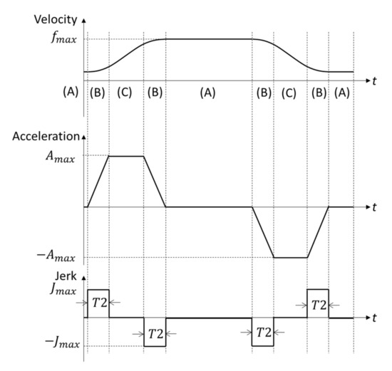
Figure 1.
S-shaped acceleration/deceleration (Acc/Dec) control for a signal block.
Generally, each axis has an allowable acceleration value that is determined according to the driving capability of its servo motor. Compared with a single block, multiple blocks of numerical control (NC) codes require one more parameter, which is given as the corner velocity [24] (Figure 2b). However, velocity discontinuity may occur when the velocity profile is distributed to each axis, as indicated in Figure 2c,d. Clearly, a higher corner velocity reduces the MT, but discontinuity can cause high acceleration and jerk for each axis as well as a large vibration in the corner.
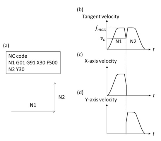
Figure 2.
Corner velocity in velocity profile: (a) a sample NC code and multiple blocks (b) tangent velocity profile (c) x-axis velocity profile (d) y-axis velocity profile.
To reduce discontinuity, the Acc/Dec after interpolation (ADAI) [12] for each axis is applied. The ADAI is a finite impulse response 25 filter with a time constant equal to Ta that smooths the acceleration and jerk profile, as displayed in Figure 3. The application of ADAI sacrifices contour accuracy and increases the MT. Table 1 reveals how the machine performance varies as the interpolation parameters change. The tradeoff among various parameter settings for the contour errors, MT, and corner vibration (CVib) motivated the current researchers to propose an optimization method based on the constructed ANN model.
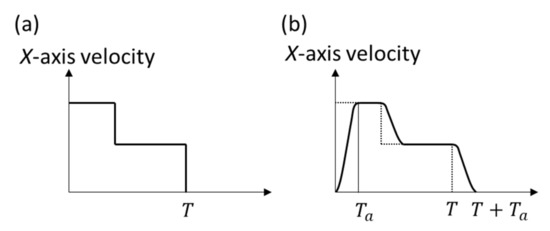
Figure 3.
(a) Velocity profiles in the Acc/Dec after interpolation (ADAI). (b) Velocity profiles out of the ADAI [25].

Table 1.
Trends in machine performance as the interpolation parameters change.
3. Experimental Procedure and Analysis Process
3.1. Experimental Designs
To establish the data-driven model, an automated acquisition system (AAS) was developed. The AAS uses the Fuji Automatic Numerical Control (FANUC) Open CNC API Specifications library (FOCAS) to capture the position command and position feedback. The tracking error and contour error can be computed accordingly. The vibration signal measured by a three-axis accelerometer (PCB 356A32 was made by PCB Piezotronics, Depew, NY, USA) is captured using National Instrument (NI) devices (NI-9234). To ensure the AAS could acquire data without operators, the library provided by NI ANSI C support was used together with the FOCAS library. The human–machine interface (HMI) program is presented in Figure 4. The program includes functions to connect the CNC controller and NI device and to execute experiments sequentially by using a designed script file that can change the values of five interpolator parameters and the total acquisition time. Here, the sampling rate for the CNC was 1000 Hz, and that for the NI-9234 was 2048 Hz.
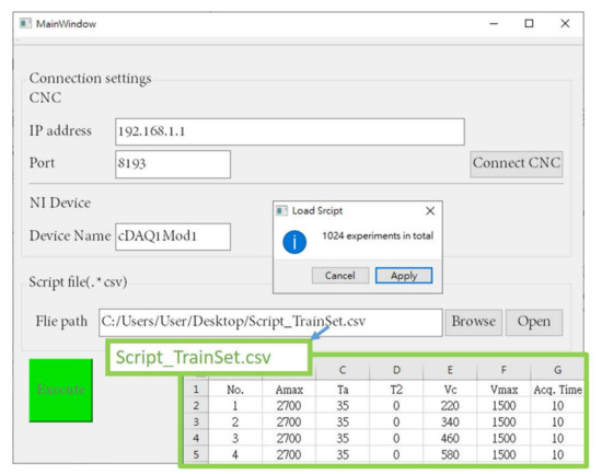
Figure 4.
Human–machine interface (HMI) of the automated acquisition system.
The experiments were conducted on a three-axis horizontal milling machine (Tongtai HA-500II was manufactured by Tongtai Machine and Tool Co., LTD., R.O.C., Kaohsiung City, Taiwan), with the three-axis accelerometer (PCB 356A32) installed on the spindle housing, as shown in Figure 5.
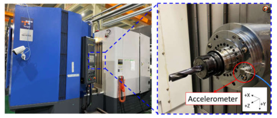
Figure 5.
Experimental machine and accelerometer setup.
To investigate the dynamic responses for setting various interpolation parameters, a FFD was adopted in this study. The design of the interpolation parameters is presented in Table 2; the values of the parameters were selected according to the various machining conditions. Each parameter, namely, , , T2, , and , was set to four different levels. In total, 1024 experiments were conducted for the FFD, and the designed parameter ranges were applied to various machining processes.
Table 2.
Levels of each interpolation parameter.
The 1024 experiments for the given trajectory discussed in Section 3 required 9 h to complete. However, the AAS could command the machine to conduct the designed trajectory and capture the data automatically without pressing the cycle-start button. Compared with the TED, the FFD obtained an enhanced ANN model; this finding is described in Section 4.2.
3.2. Preprocessing of the Data into Performance Index
In this study, the minimized cost function was selected to be the weighted sum of different performance indices. The three performance indices were the maximum contour error (MCoE), MT, and corner vibration (CVib). The captured data had to be converted into performance indices before the training process commenced.
3.2.1. Analysis of Contour Error and MT
The contour error is defined as the short distance between the desired contour and machining contour, as shown in Figure 6, where the desired contour is obtained from the G-code and the machining contour is obtained from the position feedback. The rectangular trajectory, as displayed in Figure 7, can be tested by tuning various interpolator parameters. The maximum acceleration, ADAI, time constant of the S-shaped Acc/Dec corner velocity, and maximum velocity all may have dramatic effects on corner errors, vibration, and MT. Thus, the testing trajectory in Figure 7 was applied as the machining trajectory under various interpolator parameters. For the trajectory consisting of a straight-line segment, the contour error could be computed by simply applying the point-to-line formulation.
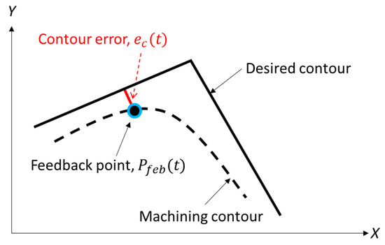
Figure 6.
Definition of contour error.
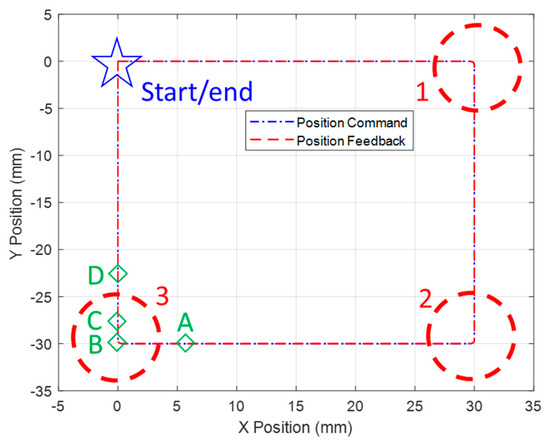
Figure 7.
Testing trajectory. (The corner 1, 2 and 3 were described in Section 3.2.1 and the period A, B, C and D were described in Section 3.2.2.).
Figure 8 reveals the contour errors of the experiment, with the , , T2, , and being given as 2700 , 35 , 0 , 220 , and 1000 , respectively. The maximum contour in corners 1, 2, and 3 was approximately 60 . The other contour errors away from the corner were much less than that of the maximum contour. On the basis of this observation, the MCoE was selected as the first performance index. The MT is also a critical factor and thus was selected as the second performance index. In this case, the MT equaled 7.361 s.
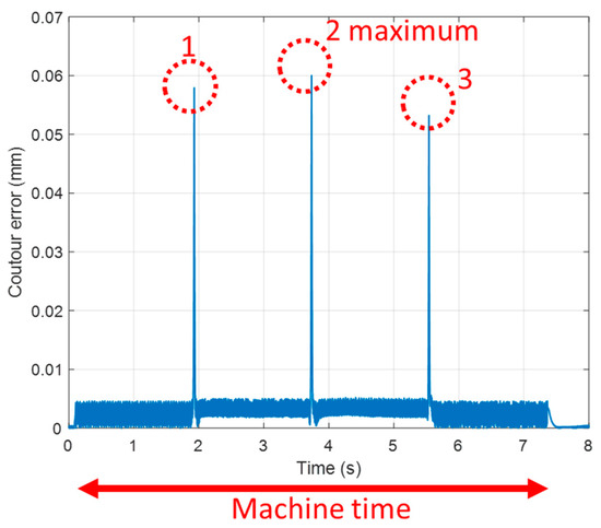
Figure 8.
Maximum contour error (MCoE) and machining time (MT) for one experiment. (The period 1, 2 and 3 were marked as the corner 1, 2 and 3 in Figure 7, respectively.)
3.2.2. Analysis of CVibs
As shown in Figure 2, the discontinuity of the velocity profile in the corner can cause a large acceleration and jerk. The vibrations in corner 3 in the x direction in Figure 9 validate the observation. The parameters of , , T2, , and used in the experiment were 2700 , 35 , 0 , 580 , and 1500 , respectively. To further analyze the vibration behavior in the corner, four periods were marked as A, B, C, and D. As indicated in Figure 2, period A corresponds to the motion of the x axis moving in a state of constant velocity. Period C is the state right after the corner as shown in Figure 7. Due to the discontinuity velocity profile as shown in Figure 2, excessive vibration might occur as shown in Figure 9. Period D corresponds to the motion for the y axis moving at a constant velocity. Because the vibration of period B corresponds to the designed Acc/Dec, the residual vibration at period C could cause machining marks in the corner. The vibration in period C was selected as the third performance index.
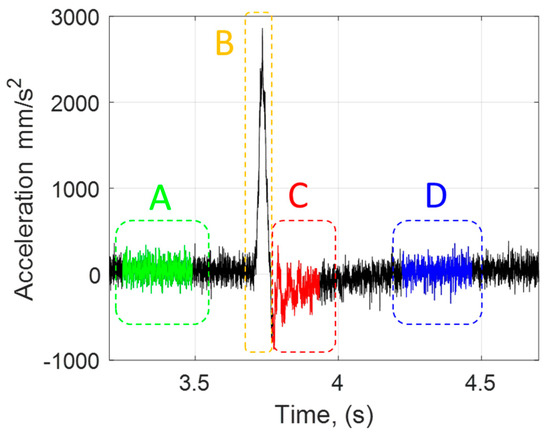
Figure 9.
Raw vibrations of the high Acc/Dec experiment. (The period A, B, C and D were marked as in Figure 7, respectively.)
To further observe the vibration behavior around the corner, the fast Fourier transform (FFT) for the periods A, C, and D was calculated (Figure 10). Four major peaks were observed at 30, 40, 116, and 426 Hz. The first natural frequency was revealed to be 30 Hz, which affects the machining process more dramatically compared with the other modes. Furthermore, the magnitude of the 30 Hz mode was highly dependent upon the interpolator parameters. The analysis of 1024 experiments revealed that the 30 Hz vibration mode can be effectively reduced by tuning the interpolation parameters, whereas the other frequency modes were less susceptible to change. Therefore, the vibration magnitude of 30 Hz was selected as the third performance index.
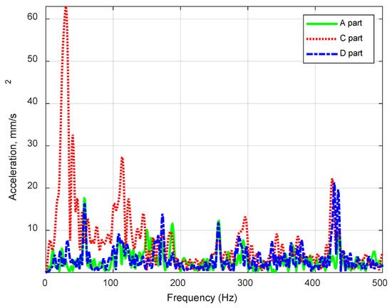
Figure 10.
Fast Fourier transform (FFT) for vibrations of periods A, C, and D in Figure 9.
4. Modeling and Optimization Concerns
The machine performance index is well known to be highly affected by Acc/Dec planning. A data-driven model is presented in this section for predicting the machine performance index. The MCoE and MT were computed from the command and position feedback, and the CVib was computed from the accelerometer. The Z-score was applied to normalize the performance index, and the BPNN was applied to establish the model and used to evaluate the testing trajectory.
4.1. Z-Score (Standard Score)
Because each dimension of the performance index is different, the accuracy of the trained model might be biased. To address this problem, a normalization and standardization process is generally used in machine learning. The Z-score is used to convert the raw data according to , where μ and are the mean and standard deviation of the population, respectively. For the testing and training data, the μ and of the MCoE were 46.08 and 21.17 , respectively. The μ and of the MT were 12.69 and 7.45 s, respectively. The μ and of the CVib were 7.62 and 6.16 , respectively.
4.2. BPNN Algorithm
A conventional BPNN algorithm [26], displayed in Figure 11, was applied to predict the machine performance indices. Several methodologies, such as [16,18], were tested, but the BPNN was the most accurate for predicting the information index and could be applied later in the optimization process with less computational burden. The architecture contained five inputs, three output elements, 20 hidden layers, and one output layer.
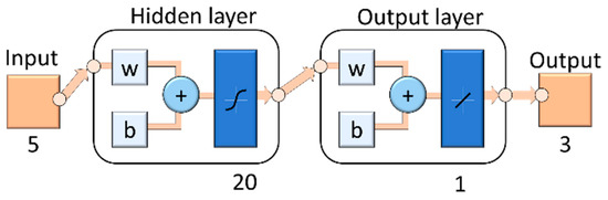
Figure 11.
Architecture of the backpropagation neural network (BPNN).
The inputs were the interpolation parameters listed in Table 2, and the outputs were the performance indices, namely, the MCoE, MT, and CVib. The training dataset was from the 1024 experiments described in Section 3, and the validation dataset comprised 64 randomly selected experiments and the parameter ranges in Table 2. Besides, 1024 experiments were conducted for the training dataset; another 64 experiments were conducted for the validation of the training model. The other four experiments were executed for testing the optimization process. A total of 1092 experiments were conducted in the study. In Table 3, the training and validation results for the root mean square error (RMSE) and maximum error (ME) are listed to demonstrate the accuracy of the trained model.
Table 3.
Training and validation results for the artificial neural network (ANN) model: the maximum contour error (MCoE) and machining time (MT) and corner vibration (CVib).
In the validation dataset, the RMSE and ME of the MCoE were 1.0976 and 5.5356 , respectively. The RMSE and ME of the MT were 0.1305 and 0.5847 s, respectively. The RMSE error was approximately 1% when a mean value of MT μ equal to 12.69 s was applied. Finally, the RMSE and ME of the CVib were 4.48 and 8.28 , respectively. The correlation coefficients of the predicted values and experimental results were calculated using the Excel CORREL function. The equation for the correlation coefficient for a two random variable array of X and Y is defined as
where and are the means of the data of x and y, respectively. The correlation coefficients of the predicted values and experimental results for the MCoE, MT, and CVib based on the validation data were 0.9984, 0.9998, and 0.9354, respectively. As indicated in the introduction, the vibration of a machine tool is extremely difficult to predict using the finite element method. The high correlation coefficients suggest the developed model is accurate for designing the interpolation parameters.
Experimental design is a crucial concern in developing data-driven models. The TED has the advantage of requiring a relatively low number of experiments, which reduces the data acquisition time. However, the results might not be as accurate as those generated through a FFD [27]. To compare the performance of the two experimental design approaches, L16() arrays—including five factors and four levels—were used in the TED in this study. Only 16 experiments were conducted with the training dataset. The RMSE and ME of the MCoE were 19.33 and 40.47 , respectively. The RMSE and ME of the MT were 2.1144 and 7.9993 s, respectively. The CVib was 13.52 and 26.12 , respectively. Thus, the accuracy of the TED-based model was much lower than that of the FFD. Although the number of experiments needed in the FFD was much higher than that in the TED, the AAS provided a convenient platform for conducting more experiments with less effort.
4.3. Design Optimization Concerns and Components of the Multi-Objective Function
After the BPNN model was developed, the next step was to define the cost function for optimization. Here, the genetic algorithm (GA) was applied to search for the optimum solution based on unconstrained functions. The GA, relying on biologically inspired operators such as selection, crossover, and mutation to generate high-quality solutions, is commonly used in nonlinear optimization problems. The GA provided the multi-objective optimization solution with the given constraints on the interpolation parameters. Here, a weighted sum approach 16 was adopted, and the objective function was given as
where f1, f2, and f3 represent the BPNN outputs, and w1, w2, and w3 are the weighting functions, respectively. The objective function with constraints is listed in Table 4. Depending on the machining process, different weightings were selected; the results are listed in Table 5. For example, if w1, w2, and w3 were set to (1, 0, 0), accuracy was the major priority. The GA algorithm determined the optimization interpolation parameters with the lowest acceleration , feedrate , and corner velocity , and the largest time constants and within the given constraints. For the weighting selected as (0, 1, 0), the major priority was MT, and the corresponding results are given in Table 6. The machine time was approximately 5 s, which was the shortest among the four cases. Generating noteworthy results that had not been reported in the literature was the priority; thus, the vibration for Case 3 was selected. In Case 3, the CVib was the lowest among the four cases, but the MT was longer than that of Case 2. Neither the MCoE or MT, nor the CVib of Case 4 achieved the highest performance among the four cases. Without the model, determining the optimization parameters was impossible.
L = w1 × f1 + w2 × f2 + w3 × f3
Table 4.
Multi-objective function and constraints following the weighted sum approach.
Table 5.
Results for optimized interpolation parameters according to the optimized mode.
Table 6.
Artificial neural network (ANN)-predicted and experimental results for MCoE, MT, and CVib.
The predicted and experimental results are listed in Table 6; these data were used to validate the accuracy of the BPNN model. Notably, the MT accuracy for all the cases was less than 3%, which is challenging to achieve without knowing the CNC kernel for the FANUC controller.
4.4. Verification by Employing a Complex Path
To apply the developed model in real machining, a complex trajectory, illustrated in Figure 12a, was tested. The trajectory, including the G01, G02, and corner errors for the conjunction of each segment, is displayed in Figure 12b–e. The interpolation parameters listed in Table 5 were used in the experiments. Clearly, contour errors generally occurred in sharp corners. The contour errors for the smooth conjunctions between G01 and G02 and from G02 to G03 in the period K5–K7 were extremely small compared with those in the period K2–K4. As expected, the MCoE for Case 1 at the peak of the period K2–K4 was the smallest, and the MCoE of Case 2 was the largest. The vibrations for Case 1 to Case 4 in the period K1 are revealed in Figure 13. Case 3 had the lowest vibration among the four cases. To further illustrate the spectrum of the vibration, FFT was conducted on the vibration signal when passing the corner; the results are presented in Figure 13b. Clearly, the CVib of Case 2 was the largest among the four cases, and that of Case 3 achieved the least vibration at the first resonance.
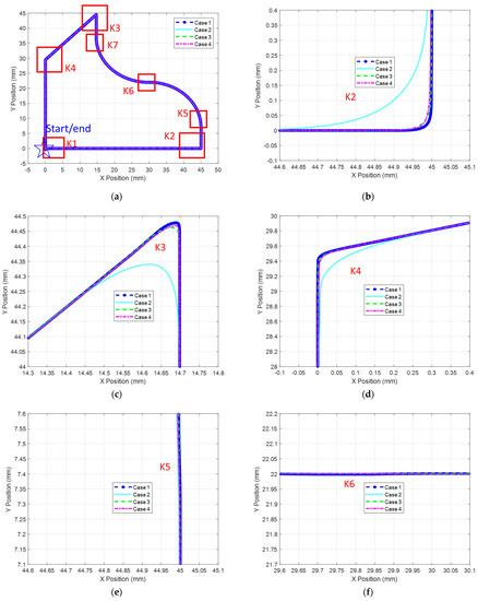
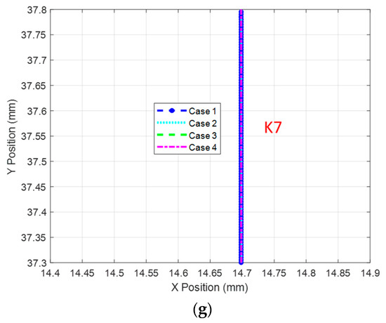
Figure 12.
Experimental contour for Cases 1 to 4: (a) overview, (b) period K2, (c) period K3, (d) period K4, (e) period K5, (f) period K6, and (g) period K7.
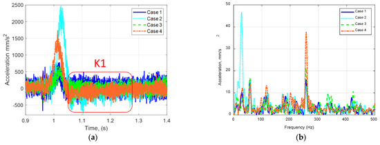
Figure 13.
(a) CVib of Case 1 to Case 4. (b) FFT result.
5. Conclusions
This study proposed an optimization algorithm for tuning the CNC interpolation parameters by considering multiple objective functions such as contour errors, the machining time, and corner vibrations. It is known that the five different parameters of , and of the interpolator can influence the objective functions significantly. For example, a higher level of acceleration will reduce the machining time and increase the contour error and corner vibrations. However, no systematic approach has been adopted to determine the optimal solutions under different machining processes. In this study, 1024 experiments were conducted, and the experimental data—the MCoE, MT, and CVib—were captured automatically and analyzed to compute the performance index. A BPNN with 20 hidden layers was applied to establish the relationship between the interpolation parameter and performance index. The correlations between the predicted values and experimental results for the MCoE, MT, and CVib were 0.9984, 0.9998, and 0.9354, respectively. Then, the GA was adopted based on the BPNN model to determine the optimized interpolation parameter. The experimental results validate the accuracy and efficiency of the proposed algorithm. With the developed optimization methodology, operators can set up the parameters systematically by selecting different weighting without a trial-and-error process. The future work will be adding the surface roughness into the performance indices such that one will be able to determine the surface quality, machining time, and contour errors simultaneously.
Author Contributions
H.-C.T., M.-S.T., C.-C.C. and C.-J.L. initiated and developed the concepts related to this research work. H.-C.T. performed the collected data for the designed experiment and analyzed the data. Both of them discussed the experimental results and developed the tuning methodology. H.-C.T. wrote the paper draft under M.-S.T. and C.-C.C.’s guidance. All authors discussed the results and commented on the manuscript. All authors have read and agreed to the published version of the manuscript.
Funding
This research was supported by the Ministry of Science and Technology (MOST), R.O.C., under the contracts MOST 108-2634-F-194-001, MOST 108-2221-E-002-156-MY3, and MOST 108-2218-E-002-071, and the Tongtai Machine & Tool Co., LTD., R.O.C.
Data Availability Statement
Not applicable.
Acknowledgments
The authors would like to thank the reviewers and editors for their suggestions.
Conflicts of Interest
The authors declare no conflict of interest.
References
- Lyu, D.; Liu, Q.; Liu, H.; Zhao, W. Dynamic error of CNC machine tools: A state-of-the-art review. J. Adv. Manuf. Technol. 2020, 106, 1869–1891. [Google Scholar] [CrossRef]
- Cheng, M.Y.; Lee, C.C. Motion controller design for contour-following tasks based on real-time contour error estimation. IEEE Tran. Ind. Electron. 2007, 54, 1686–1695. [Google Scholar] [CrossRef]
- Sencer, B.; Ishizaki, K.; Shamoto, E. High speed cornering strategy with confined contour error and vibration suppression for CNC machine tools. CIRP Ann. 2015, 64, 369–372. [Google Scholar] [CrossRef]
- de Jesus Rangel-Magdaleno, J.; de Jesus Romero-Troncoso, R.; Osornio-Rios, R.A.; Cabal-Yepez, E.; Dominguez-Gonzalez, A. FPGA-based vibration analyzer for continuous CNC machinery monitoring with fused FFT-DWT signal processing. IEEE Tran. Instrum. Meas. 2010, 59, 3184–3194. [Google Scholar] [CrossRef]
- Sangwan, K.S.; Saxena, S.; Kant, G. Optimization of machining parameters to minimize surface roughness using integrated ANN-GA approach. Procedia. Cirp. 2015, 29, 305–310. [Google Scholar] [CrossRef]
- Zhang, J.Z.; Chen, J.C.; Kirby, E.D. Surface roughness optimization in an end-milling operation using the Taguchi design method. J. Mater. Process. Technol. 2007, 184, 233–239. [Google Scholar] [CrossRef]
- Benardos, P.G.; Vosniakos, G.C. Predicting surface roughness in machining: A review. J. Mach. Tools Manuf. 2003, 43, 833–844. [Google Scholar] [CrossRef]
- Alonso, F.J.; Salgado, D.R. Analysis of the structure of vibration signals for tool wear detection. Mech. Syst. Signal Proc. 2008, 22, 735–748. [Google Scholar] [CrossRef]
- Okwudire, C.; Ramani, K.; Duan, M.A. trajectory optimization method for improved tracking of motion commands using CNC machines that experience unwanted vibration. CIRP Ann. 2016, 65, 373–376. [Google Scholar] [CrossRef]
- Bringmann, B.; Maglie, P. A method for direct evaluation of the dynamic 3D path accuracy of NC machine tools. CIRP Ann. 2009, 58, 343–346. [Google Scholar] [CrossRef]
- Erkorkmaz, K.; Altintas, Y. High speed CNC system design. Part III: High speed tracking and contouring control of feed drives. J. Mach. Tools Manuf. 2001, 41, 1637–1658. [Google Scholar] [CrossRef]
- Tsai, M.S.; Huang, Y.C. A novel integrated dynamic acceleration/deceleration interpolation algorithm for a CNC controller. J. Adv. Manuf. Technol. 2016, 87, 279–292. [Google Scholar] [CrossRef]
- Altintas, Y.; Brecher, C.; Weck, M.; Witt, S. Virtual machine tool. CIRP Ann. 2005, 54, 115–138. [Google Scholar] [CrossRef]
- Zain, A.M.; Haron, H.; Sharif, S. Prediction of surface roughness in the end milling machining using Artificial Neural Network. Expert. Syst. Appl. 2010, 37, 1755–1768. [Google Scholar] [CrossRef]
- Chiu, H.W.; Lee, C.H. Prediction of machining accuracy and surface quality for CNC machine tools using data driven approach. Adv. Eng. Softw. 2017, 114, 246–257. [Google Scholar] [CrossRef]
- Konak, A.; Coit, D.W.; Smith, A.E. Multi-objective optimization using genetic algorithms: A tutorial. Reliab. Eng. Syst. Saf. 2006, 91, 992–1007. [Google Scholar] [CrossRef]
- Tsai, J.T.; Chou, J.H.; Liu, T.K. Tuning the structure and parameters of a neural network by using hybrid Taguchi-genetic algorithm. IEEE Trans. Neural. Netw. 2006, 17, 69–80. [Google Scholar] [CrossRef] [PubMed]
- Asiltürk, I.; Akkuş, H. Determining the effect of cutting parameters on surface roughness in hard turning using the Taguchi method. Measurement 2011, 44, 1697–1704. [Google Scholar] [CrossRef]
- Urbikain, G.; Campa, F.J.; Zulaika, J.J.; De Lacalle, L.N.L.; Alonso, M.A.; Collado, V. Preventing chatter vibrations in heavy-duty turning operations in large horizontal lathes. J. Sound Vib. 2015, 340, 317–330. [Google Scholar] [CrossRef]
- Garitaonandia, I.; Fernandes, M.H.; Albizuri, J. Dynamic model of a centerless grinding machine based on an updated FE model. J. Mach. Tools Manuf. 2008, 48, 832–840. [Google Scholar] [CrossRef]
- Mi, L.; Yin, G.F.; Sun, M.N.; Wang, X.H. Effects of preloads on joints on dynamic stiffness of a whole machine tool structure. J. Mech. Sci. Technol. 2012, 26, 495–508. [Google Scholar] [CrossRef]
- Erkorkmaz, K.; Altintas, Y. High speed CNC system design. Part I: Jerk limited trajectory generation and quintic spline interpolation. J. Mach. Tools Manuf. 2001, 41, 1323–1345. [Google Scholar] [CrossRef]
- Suh, S.H.; Kang, S.K.; Chung, D.H.; Stroud, I. Theory and Design of CNC Systems; Springer Science & Business Media: London, UK, 2008. [Google Scholar]
- Jahanpour, J.; Alizadeh, M.R. A novel acc-jerk-limited NURBS interpolation enhanced with an optimized S-shaped quintic feedrate scheduling scheme. J. Adv. Manuf. Technol. 2015, 77, 1889–1905. [Google Scholar] [CrossRef]
- Chen, C.S.; Lee, A.C. Design of acceleration/deceleration profiles in motion control based on digital FIR filters. J. Mach. Tools Manuf. 1998, 38, 799–825. [Google Scholar] [CrossRef]
- Hagan, M.T.; Demuth, H.B.; Beale, M.; De Jesus, O. Neural Network Design Boston; PWS-Kent: Plaza Boston, MA, USA, 1996; pp. 11–17. [Google Scholar]
- Medan, N.; Lobontiu, M.; Nagy, S.R.; Dezső, G. Taguchi versus full factorial design to determine the equation of impact forces produced by water jets used in sewer cleaning. In Proceedings of the MATEC Web of Conferences, Iasi, Romania, 24–27 May 2017; Volume 112, p. 03007. [Google Scholar]


Publisher’s Note: MDPI stays neutral with regard to jurisdictional claims in published maps and institutional affiliations. |
© 2021 by the authors. Licensee MDPI, Basel, Switzerland. This article is an open access article distributed under the terms and conditions of the Creative Commons Attribution (CC BY) license (http://creativecommons.org/licenses/by/4.0/).