Article

Intensity Measure Based on a Smooth Inelastic Peak Period for a More Effective Incremental Dynamic Analysis

by
Juan Carlos Vielma
1,*,
Maria Cristina Porcu
2 and
Nelson López
3
1
Civil Engineering School, Pontificia Universidad Católica de Valparaíso, Valparaíso 2340000, Chile
2
Department of Civil Engineering, Environmental Engineering and Architecture, University of Cagliari, 09131 Cagliari, Italy
3
Structural and Geotecnic Departament, Pontificia Universidad Católica, Santiago 7820436, Chile
*
Author to whom correspondence should be addressed.
Appl. Sci. 2020, 10(23), 8632; https://doi.org/10.3390/app10238632
Submission received: 20 October 2020 / Revised: 28 November 2020 / Accepted: 30 November 2020 / Published: 2 December 2020

Abstract

:
The Incremental Dynamic Analysis (IDA) assesses the global collapse capacity of a structure by plotting its maximum inelastic response, obtained through a non-linear time-history analysis, versus the scaled intensity of different input earthquakes. The seismic intensity is often measured through the spectral acceleration at the fundamental elastic period. However, this can produce highly variable results. An alternative method is presented in this paper that relies on the elongated period, calculated either from the Fourier spectrum of the acceleration at a target building point (inelastic peak period) or from a smooth Fourier spectrum (inelastic smooth peak period). By referring to a reference reinforced concrete building and to a set of 10 spectrum-consistent earthquakes, the paper presents the results of a wide investigation. First, the variation in the elongated period as a function of the seismic intensity is discussed. Then, the effectiveness of the proposed method is assessed by comparing the IDA curves to those obtained through the elastic period or through approximate values of the elongated period given in the literature. The results show that the alternative IDA procedure generates curves with less-dispersed collapse thresholds. A statistical analysis shows significant improvements in the results when the inelastic smooth peak period is adopted.

1. Introduction

Non-linear analyses are the most accurate approach for assessing the seismic behavior of civil structures, since the current codes highly encourage post-elastic dissipative behavior under strong earthquakes. Non-linear static analysis based on horizontal static loads with gradually increasing intensity (pushover analysis) is very commonly applied to ascertain the inelastic capacity of a structure until its collapse [1,2]. On the other hand, non-linear time-history analysis under spectrum-consistent earthquakes may be very useful for studying the evolution of the seismic demand on a given structure [3,4,5]. Stemming from the concept of incremental seismic actions typical of pushover analysis, incremental dynamic analysis (IDA) is a type of non-linear analysis technique under scaled ground accelerations that is currently perceived as the most advanced tool for assessing the seismic response of structures. In the guidelines published by the Federal Emergency Management Agency (FEMA) [6,7], IDA is presented as the fundamental basis with which to determine the performance factors of new types of structures, as well as to obtain the collapse thresholds of existing structures while considering the variability of seismic records. Many authors have carried out IDA to obtain the performance of different kinds of new and existing structures [8,9,10,11,12,13,14,15,16,17]—even structures equipped with dissipation or isolation devices [18].
However, some disadvantages still affect the accuracy of IDA, particularly the high record-to-record variability of the curves representing the maximum demand on a given building at different scaled seismic intensities. While the engineering demand parameter is usually taken as the maximum interstory drift ratio of a building, how to choose the most suitable measure of the scaled seismic intensity remains highly debated and is crucial for ensuring that the IDA procedure is sufficiently effective [19,20,21,22,23,24,25,26,27,28,29].

1.1. Background

The unified procedure usually adopted to carry out IDA was originally formulated by Vamvatsikos and Cornell in [19]. Their approach is based on a simple transformation of the amplitude of a reference “as-recorded” accelerogram a 1 ( t ) that is uniformly scaled up or down by a scale factor (SF), denoted λ , so that λ [ 0 , + ] :   a λ = λ   a 1 . In the elastic range, scaling the accelerogram corresponds to scaling the elastic response spectrum or, equivalently, scaling the Fourier amplitude spectrum while keeping the phase information intact.
By successively integrating the non-linear motion equations under a given earthquake, which is scaled at each iteration with a different SF, the progressive performance of a structure can be assessed from the elastic to the inelastic range until collapse. To characterize the intensity of the scaled ground motion, a parameter is adopted, namely, the intensity measure ( I M ), which depends on the unscaled accelerogram a 1 and increases with the SF λ , that is, I M = f a 1 ( λ ) [19]. On the other hand, an engineering demand parameter, namely, the damage measure ( D M ) should be chosen to assess the structural responses at different seismic intensity levels.
For each given accelerogram, a curve plotting the values of D M as a function of I M can be built. However, a single-record IDA study cannot fully capture the seismic capacity of a building. Therefore, a consistent set of records should be considered to perform a complete multi-record IDA analysis. FEMA (Federal Emergency Management Agency) codes [6,7] recommend the use of a group of earthquakes registered in the Pacific Earthquake Engineering Research Center (PEER) database. A group of curves can thus be obtained for multi-record IDA analysis, which is expected to give a thorough understanding of the structural demand for different intensity levels of seismic action.
Although different D M values can be chosen to assess the seismic demand under earthquakes of different intensities, the maximum interstory drift ratio is widely adopted as one of the most significant parameters. In contrast, the choice of the most appropriate I M value is still much debated (see, e.g., [17,18,19,20,21,22,23,24,25]). The reason for this debate is that a suitable choice of I M should account for both the seismological characteristics of the ground motion (which are typically related to the statistical properties of seismic hazard analysis) and the structural response features of the considered building (which can be estimated through the maximum values of the given target engineering parameters). However, due to record-to-record variability, comparatively high scatter in the structural responses under different reference accelerograms may affect the efficiency (the ability to predict the structural capacity independent of the selected record), the sufficiency (no other ground motion information is needed) and the scaling robustness (the ability of the SF to predict the structural response) of I M [20,21,22,23,24,25] and, consequently, the effectiveness of the whole IDA procedure.
Several I M parameters have been proposed in the literature with the aim of meeting the above requirements and reducing the dispersion of the results under different ground motions. Such parameters refer, for instance, to the peak ground acceleration (PGA), peak ground velocity, peak ground displacement, effects of the spectral shape and ground motion duration, Arias intensity, Housner intensity, spectral response, and yield reduction R-factor [17,18,19,20,21,22,23]. Nevertheless, a common choice for I M is the spectral acceleration taken at the structure’s first-mode period; for a damping factor ξ = 5 % , the spectral acceleration is S a ( T 1 , ξ ). The elastic response spectrum is broadly recognized as an excellent tool to link the seismological characteristics of an earthquake to the seismic demand in single-degree-of-freedom systems.
On the other hand, assuming S a ( T 1 , ξ ) to represent I M may involve some disadvantages [19], for instance, due to (i) neglecting the contributions from higher vibration modes, (ii) lengthening of the fundamental period associated with the non-linear hysteretic behavior of the structure [23], and (iii) the spectral shape bias occurring when using high SFs [26,27].
Even for structures dominated by the first vibration mode, the non-linearity of the response has crucial impacts [23], and thus, the intensity measures based on such non-linear responses are shown to be more efficient in reducing the variability of the seismic demand [28]. In fact, global stiffness degradation and strength reduction typically occur in reinforced concrete (R/C) buildings due to the local cracking of concrete and yielding of reinforcing bars during earthquake loading reversals; such deterioration changes the dynamic modal characteristics of the system, which can also be exploited to detect local damage during structural health monitoring [30,31]. Structures typically exhibit a change in the natural period when they deform widely in the plastic range, where the “inelastic” (apparent) period is usually longer than the elastic period (relevant to the undamaged structure) [32]. In particular, the vibration period of R/C buildings was found to be highly elongated due to plastic deformation during severe ground motions (from 50 to 70% up to 100 to 130%) [32].

1.2. Recommended Values of the “Inelastic” Period for the Earthquake Intensity Measure

The inelastic elongated fundamental period T i n is a key parameter for establishing a rigorous evaluation of structural performance into the non-linear regime; for this reason, T i n can represent the intensity measure required for IDA better than the elastic fundamental period T e l . Therefore, I M could be evaluated by entering the earthquake response spectrum with the inelastic period T i n instead of the elastic period T e l .
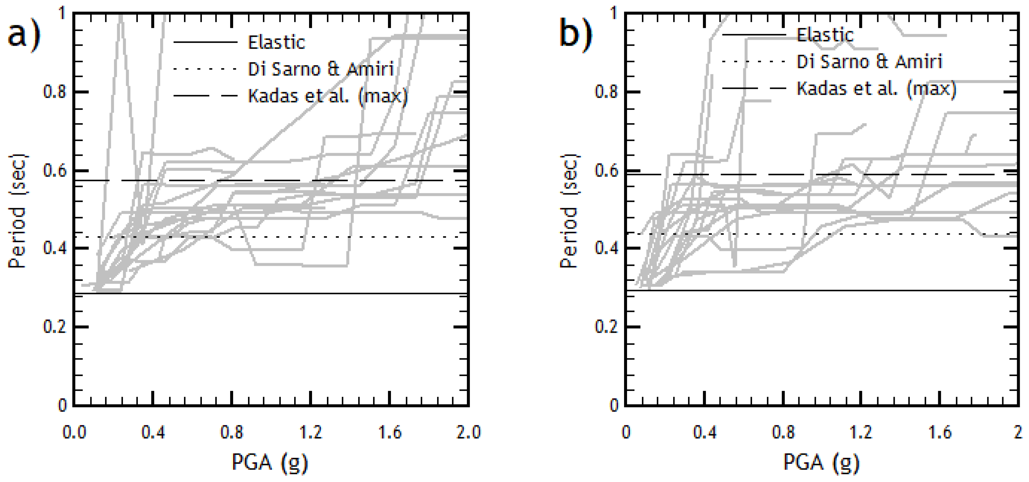
Evaluating the lengthening of the period is still an open issue in earthquake engineering. Based on many numerical investigations, some empirical formulas have been proposed in the literature. Kadas et al. [24] studied over 100 ground motion records and proposed the following relationship between the elastic initial period T e l and the inelastic final period T i n [24]:
T i n = 1.07   T e l   ( S a ( T e l ) A y ) 0.45 2   T e l ,
where A y is the yield spectral acceleration. Note that Equation (1) limits the value of the elongated period to twice the elastic period.
To predict the value of the fundamental period shift ratio ( T i n / T e l ) of R/C structures, Di Sarno and Amiri [33] provided the following formula:
T i n T e l = 3.6 2.367 exp ( 0.006   T e l 2.412 )
The above relation produces values of T i n ranging from approximately 3.6   T e l (for very rigid oscillators) to 1.23   T e l (for flexible oscillators). Some corrective parameters are also given in [33] to adjust the “reference” values obtained from Equation (2) to account for some deterioration effects.
By referring to one-degree-of-freedom oscillators equivalent to the considered multi-degree-of-freedom systems, Katsanos et al. [32] derived the value of the inelastic period at the maximum amplitude of the Fourier spectrum relevant to the structural acceleration under each scaled earthquake. Both regular and irregular multi-story buildings were considered in [32] under hundreds of recorded earthquakes, two different hysteretic rules, and 11 scaling factors (PGA reaching up to 1.7 g). The results presented by Katsanos et al. [32] showed that the shift ratio T i n T e l is typically lower than 1.7. It should be noted, however, that such results were obtained by carrying out in-plane analyses on the equivalent one-degree-of-freedom oscillators.

1.3. Basic Assumptions and Purposes of the Study

The present paper proposes to evaluate the intensity of a scaled ground motion by referring to the earthquake spectral acceleration taken at the inelastic elongated period, the latter being obtained from a time-history analysis. Two different methods are proposed to derive the elongated period. The first approach derives an inelastic peak period T inP from the Fourier amplitude spectrum of the acceleration of a building’s reference point; the second method obtains an inelastic smooth peak period T i n S P from the smooth Fourier spectrum derived from the original spectrum by applying a suitable filtering technique.
In practice, the I M parameter is calculated by means of the spectral acceleration (for a dampening factor ξ = 5 % ) taken at the structure’s elongated period T i n instead of the elastic fundamental period T e l = T 1 . The value of T i n is derived from the Fourier amplitude spectrum (obtained through the fast Fourier transform) relevant to the structural acceleration taken at the center of gravity of the building’s roof.
Two alternative strategies will be adopted to obtain the elongated period. The first strategy derives the value of T i n P = 2 π / ω i n P from the predominant frequency ω i n P taken at the peak amplitude of the Fourier spectrum (red diagram in Figure 1). This period will hereafter be referred to as the “inelastic peak period”. The following formula is thus considered to obtain the value of I M in this case:
I M i n P   =   S a ( T i n P , 5 % ) ,
It should be observed, however, that the higher the scale factor of the input record, the more difficult it may be selecting with confidence the right value of the predominant frequency ω i n P from the Fourier amplitude spectrum, due to the several peaks that may occur in the range where the predominant frequency falls (see Figure 1). This was found to lead to the inconsistency of the values of a period that does not coherently elongate as the intensity of the scaled ground motion increases, as shown in the following sections. Therefore, a second strategy to obtain the elongated period has been considered. It is based on a smooth Fourier amplitude curve derived from the original Fourier spectrum by applying a suitable filtering technique (blue curve in Figure 1). The value of the predominant frequency ω i n S P is taken at the curve peak of the smooth Fourier spectrum, and the elongated period T i n S P = 2 π / ω i n S P is obtained accordingly. This period will hereafter be referred to as the “inelastic smooth peak period”. By referring to T i n S P , the value of I M can be obtained as follows:
I M i n S P   =   S a ( T i n S P , 5 % ) .
In the present study, the smooth Fourier spectrum has been obtained by applying an appropriate “smoothing window” in the range 0–25 Hz, which is the range where the fundamental frequencies of buildings typically fall. The smoothing window S w is determined according to:
S w = 1 ( f c   Δ t ) ,
where, f c is the cut-off frequency of the window while Δ t is the time step of the acceleration record.
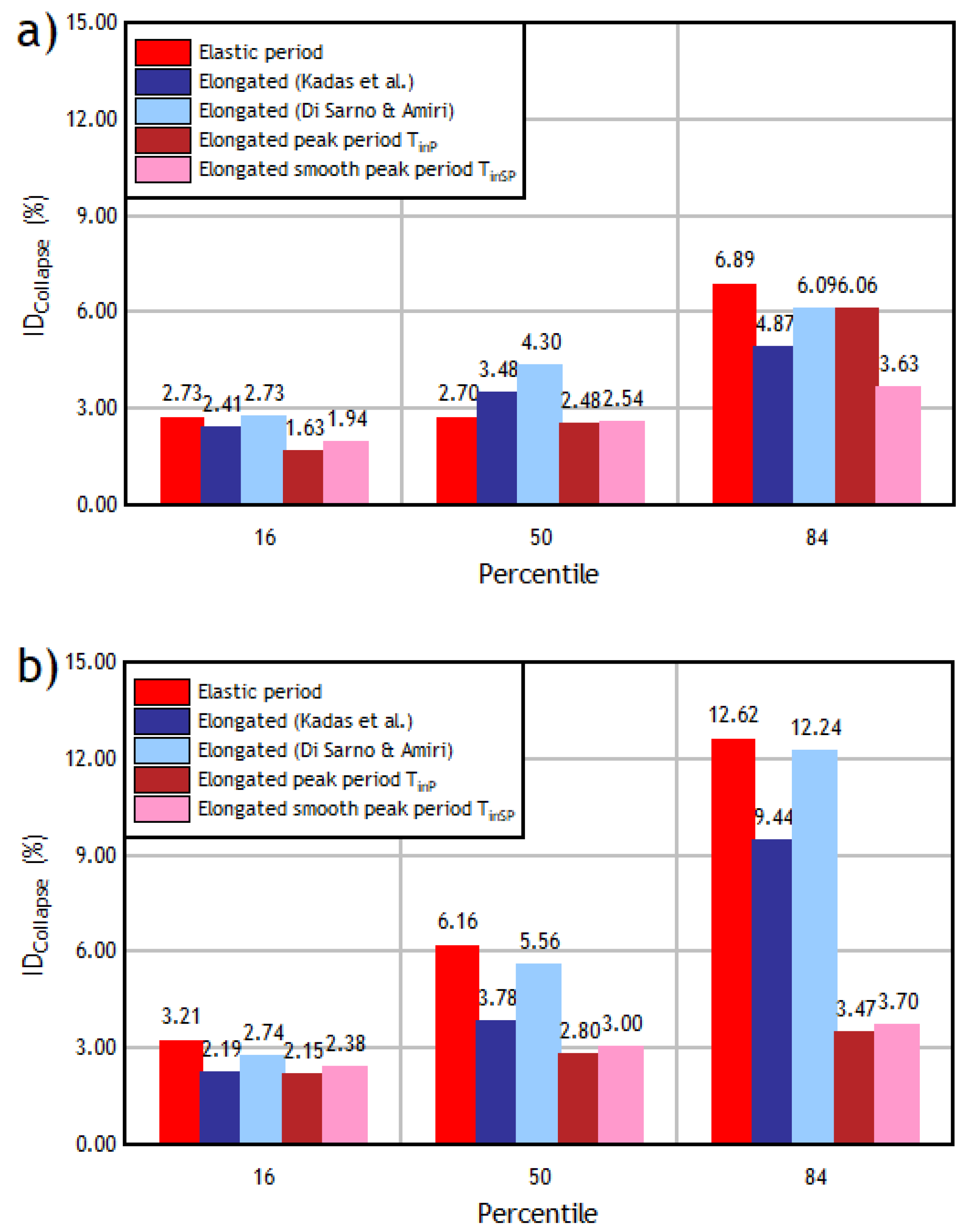
The aim of this paper is to assess whether and to what extent the adoption of either the intensity measure introduced in Equation (3) or that in Equation (4) can lead to an improvement of the IDA procedure, by reducing the dispersion of curves and improving the reliability of the results compared to other literature methods. For this purpose, the results of an extensive numerical investigation are presented to compare the IDA curves derived by entering the response spectrum with different values of the period: the elastic fundamental period; two values of the inelastic period, namely those in Equations (1) and (2); and the two values of the inelastic elongated period, namely T i n P and T i n S P , proposed in this paper.

2. Procedure for Obtaining IDA Curves by Referring to the Elongated Period ( T i n P or T i n S P )

2.1. Procedure Description

Based mainly on the classical formulation [19], an alternative procedure is proposed herein to determine the IDA curves. The proposed approach considers the I M parameter given either by Equation (3) or Equation (4). Both the inelastic peak period T i n P and the inelastic smooth peak period T i n S P are considered to check which produces better results within the IDA procedure.
The following eight steps are followed to carry out the alternative procedure proposed herein, as summarized in Figure 2.
  • Step 1. A group of uniformly increasing S F s are selected.
  • Step 2. A set of strong accelerograms (two horizontal components for each earthquake) are chosen.
  • Step 3. For any considered ground motion and for each S F , the scaled x- and y-accelerations are obtained.
  • Step 4. The scaled components of the ground motion are applied in the x- and y- directions to perform the time-history analysis.
  • Step 5. The acceleration at the center of gravity of the building’s roof is obtained through the time-history analysis.
  • Step 6a. The Fourier amplitude spectrum of the acceleration at the center of gravity is obtained, and the frequency at the maximum spectral amplitude is taken (see the red curve in Figure 1). From this frequency value, the period T i n P is calculated.
  • Step 6b. A smooth Fourier spectrum is derived from the original spectrum by applying a suitable filtering technique. The value of the predominant frequency is taken at the peak of the smooth curve (see the blue curve in Figure 1), and the corresponding elongated period T i n S P is found.
  • Step 7a. The response acceleration spectrum (with 5% critical damping) is entered with T i n P , and the spectral acceleration S a ( T i n P , 5 % ) is obtained. The intensity measure is thus calculated according to Equation (3).
  • Step 7b. The earthquake acceleration spectrum (with 5% critical damping) is entered with T i n S P , and the spectral acceleration S a ( T i n S P , 5 % ) is obtained. The intensity measure ( I M ) is thus calculated according to Equation (4).
  • Step 8. The parameter chosen to quantify the demand on the structure ( D M ) is obtained from the time-history analysis for each of the considered cases. The intensity measure I M is then plotted versus the demand measure D M to obtain the IDA curve.
Please note that Steps 6 and 7 are divided into one of two components to consider either the inelastic peak period T i n P or the inelastic smooth peak period T i n S P .
In the present study, the maximum interstory drift ratio ( I D m a x ) is adopted as the damage measure D M :
D M = I D m a x ,
As is usually assumed in the literature [19]. Once the values of I M and D M are both given, a point is drawn on the diagram where the IDA curves will be displayed. The procedure will be carried out repeatedly from Steps 3 to 8 until all the points of each single-record curve are obtained. Then, the algorithm will continue iterating to obtain the curves for the other ground motions in the set. In the present case, a multi-record IDA diagram is obtained for each of the two different inelastic elongated periods.

2.2. Reference Building to Test the Efficacy of the Method

The 3D two-story R/C building considered in the present investigation is schematically represented in Figure 3. All the structural details of this building are given in [2,3]. The seismic behavior of this building, designed according to an old Italian regulation, was assessed in [2,3], where the effectiveness of the seismic retrofit of the structure with fiber-reinforced polymer (FRP) was also evaluated. Non-linear time-history analyses (with spectrum-consistent earthquakes) were performed in [2], while the results of both pushover analysis and standard multi-record IDA were presented in [3].
The building has a rectangular plan (9.80 m × 15.50 m) with a fixed elevation height between floors (3.00 m) and fixed column sections (0.40 m × 0.40 m). An exterior R/C staircase gives the structure an irregular configuration. The slabs are ribbed in the y-direction, which defines two types of frames: frames that support predominantly seismic loads (in the y-direction) and frames that support both gravitational and seismic loads (in the x-direction). The characteristics of the structural materials are shown in Table 1. Further details about the building geometry, its steel reinforcement, and the seismic retrofit with FRP can be found in [2,3].
A 3D finite element model was implemented with SeismoStruct [34], and the building non-linear behavior was introduced through a distributed plasticity model (fiber model). Each element section was split into at least 200 fibers. Structural members were divided into four elements to identify different steel confinement zones, while the areas wrapped by FRP sheets to improve the member behavior (namely, at the ends of the ground-floor columns, see Figure 3) are considered separately, cf. [2,3]. The constitutive models of Mander et al. [11] and Menegotto and Pinto [12] were adopted for concrete and reinforcing steel, respectively. The properties of the first six modes (namely, mode type, frequency, period, effective mass in the x- and y- direction) of the building are provided in Table 2.

2.3. Set of Spectrum-Consistent Records

A set of severe ground motions compatible with the seismic conditions at the building’s location (Messina, Italy) was considered in the present investigation. Related to the building location, the design response spectrum for the no-collapse requirement (horizontal component) was considered according to Eurocode 8 [35] and Italian code [36]. Figure 4 plots this design spectrum (black curve) and the parameters adopted to obtain it. Consistent with this reference design response spectrum, 10 pairs of accelerograms were considered, some characteristics of which are listed in Table 3. In particular, the earthquake name, the date, the station identifier, the moment magnitude M w , the epicentre distance and the peak ground acceleration (PGA) are provided in the table. Note that seven of the selected accelerograms are taken from a European database and correspond to near-source earthquakes with a moderate moment magnitude M w ; they are obtained by means of REXEL software [37] according to EC8 [36]. The remaining three ground motions listed in Table 3 are near-intermediate source Chilean records obtained through SeismoSpect [38]. The response spectra of the 10 couples of records (light blue curves) with their average spectrum (blue curve) are plotted in Figure 4 together with the reference design spectrum (black).
In the present investigation, the seismic records have been scaled through non-negative scale factors S F , according to the approach proposed in Vamvatsikos and Cornell [19]. Starting from 0.3, the scale factors have been progressively increased every 0.3 until the dynamic response reached the collapse threshold defined in [19].

2.4. Inelastic Period vs. PGA

The PGA of a scaled record may be an effective measure of the seismic intensity. As a function of the PGA of the scaled accelerograms considered in the present study (Table 2), the values of the inelastic peak period T i n P obtained from the Fourier amplitude spectrum relevant to the acceleration of the center of gravity of the building’s roof are plotted in Figure 5a,b for the x- and y-directions, respectively. The diagrams in Figure 5 show very abrupt changes in the inelastic peak period curves (sharp increases and decreases) regardless of the considered record and at both low and high PGA values.
Similar diagrams for the inelastic smooth peak period T i n S P are provided in Figure 6a,b. These figures show a much more gradual growth of T i n S P for increasing PGA values. While guaranteeing that the predominant frequency is found in the frequency band containing the highest Fourier amplitudes, the smooth Fourier spectrum avoids abrupt changes in the period (see the blue curve in Figure 1), which leads to a more suitable relationship between the elongated structural period and the intensity measure, namely, the PGA, of the earthquake (Figure 6).
A comparison between Figure 5 and Figure 6 highlights that much more regular curves are obtained when considering the smooth peak period T i n S P instead of the peak period T i n P . Furthermore, the curves in Figure 6 show a slow and gradual increment in the elongated inelastic period as the seismic intensity increases. A smooth transition of the period is an expected occurrence in a structure subjected to gradually scaled accelerograms.
As obtained from a modal analysis, the values of the elastic fundamental period of the building in the x-direction ( T e l x = 0.288 s) and in the y-direction ( T e l y =   0.292 s) are plotted for comparison in Figure 5 and Figure 6 (solid horizontal lines). For very low PGA values, for instance, lower than 0.3 g (when the structure has not yet entered or has only just entered the plastic range), the value of the period taken from the Fourier amplitude spectrum should be very close to the fundamental elastic period. In contrast, Figure 5 and Figure 6 demonstrate that the conventional periods determined by modal analysis are often (even significantly) lower than T i n P and T i n S P determined by means of time-history analysis and the Fourier spectrum-based procedures.
The estimates of the inelastic period given by Kadas et al. [24] (see Equation (1)) and by Di Sarno and Amiri [32] (see Equation (2)) are also displayed in Figure 5 and Figure 6 (dashed and dotted lines, respectively). The maximum value allowed by Equation (1), T i n = 2 T e l , is considered for comparison; although being an upper limit, this value is found to underestimate the actual elongated period in many cases when both the peak period and the smooth peak period are considered (see Figure 5 and Figure 6). On the other hand, the inelastic period estimated by Di Sarno andAmiri (in the present case, T i n ~ 1.5 T e l ) is almost always defective (at least for PGA > 0.4 g) with respect to the values T i n P and T i n S P calculated through the non-linear time-history analysis and Fourier spectrum-based methods. Moreover, EC8-Part 1 [36] and ASCE/SEI 7-10 [39] suggest estimating the elongated inelastic period as 2 T e l and 1.5 T e l , respectively [32].

3. Assessing the Effectiveness of the Proposed IDA Procedure

The effectiveness of the IDA procedure proposed in Section 2.1 will be assessed by comparing it with two approaches: the standard procedure that refers to the elastic period and the procedure that refers to literature values of the elongated period calculated according to Equation (1) or to Equation (2). First, the I M and D M values are compared through different percentiles. Subsequently, the dispersion achieved by both the I M and the D M is analyzed by comparing the standard deviations and the coefficient of variation of the set of IDA curves corresponding to each direction of analysis.
The intensity measure will be given by the ξ = 5 % damped spectral acceleration at the structure’s first-mode period, that is, I M = S a ( T 1 , 5 % ). The value of T 1 will be considered either as the elastic fundamental period T e l (standard IDA procedure) or as the elongated inelastic period T i n , estimated following Kadas et al. [24] or Di Sarno and Amiri [32] or calculated as proposed in this paper (alternative IDA procedure).
According to Equation (6), the maximum interstory drift ratio of the building, referred to as I D m a x , was adopted as the indicator of the maximum demand on the structure (the D M parameter). All analyses performed herein were referenced to the two-story building displayed in Figure 3 and to the set of spectrum-consistent earthquakes described in Table 2.

3.1. Standard IDA Procedure Based on the Elastic Fundamental Period

Referring to the aforementioned building and spectrum-consistent earthquakes, a standard IDA investigation was carried out by adopting I M = I M e l = S a ( T e l , 5 % ), where T e l = T 1 is the elastic fundamental period of the structure and D M = I D m a x . The IDA curves obtained are displayed in Figure 7a,b. The plots show a rather high degree of dispersion of D M for a given I M , which indicates that the chosen I M parameter is not effective [19]. Hence, considering the elongated inelastic period instead of the elastic fundamental period might be a better choice, leading to curves with less dispersion.

3.2. IDA Curves Obtained Through Approximate Values of the Elongated Period

The results obtained by calculating the IM parameter in reference to the approximate values of the elongated fundamental period obtained from Equations (1) and (2) [24,33], are presented in this section. Figure 8 shows the IDA curves obtained by considering T i n = 2 T e l , which is the upper value proposed by Kadas et al. [24] (see Equation (1)), while the curves derived through the approximate value given by Di Sarno and Amiri [33] (see Equation (2)) are plotted in Figure 9. Despite referring to the inelastic period, the diagrams in Figure 8 and Figure 9 still show a rather high scatter because the inelastic periods estimated by the methods of Kadas et al. and Di Sarno and Amiri are constants that can greatly differ from the actual values, as also highlighted by the diagrams in Figure 5 and Figure 6.

3.3. IDA Curves Obtained through T inP and T inSP

References will now be made to the values of the inelastic period proposed in this study, namely, T i n P and T i n S P , which are derived from the Fourier amplitude spectrum and from the smooth Fourier spectrum, respectively. Figure 10 shows the IDA curves obtained when considering the intensity measure given by Equation (3), while the curves in Figure 11 are relevant to the intensity measure provided by Equation (4).

3.4. Comparison of the Results

Figure 7, Figure 8, Figure 9, Figure 10 and Figure 11 show that D M is a non-monotonic function of I M ; the curves often display a twisting pattern with both softening and (counterintuitively) hardening behaviors. Such a trend is also typical for the IDA curves when other choices of D M and I M are made, as reported in [19]. Moreover, the curves obtained for different records tend to provide rather dispersed results.
Comparing the graphs in Figure 7, Figure 8, Figure 9, Figure 10 and Figure 11 almost always reveals more marked scatter in the x-direction with respect to the y-direction regardless of the value of the period (elastic or inelastic, approximated or rigorously calculated). If a reference to the elongated period is made, however, the scatter generally reduces, even if referring to the values of the elongated period does not significantly improve the effectiveness of the IDA procedure.
In contrast, when more rigorous values of the elongated inelastic period are accounted for, namely, T i n P and T i n S P , the IDA curves exhibit less dispersion (see Figure 10 and Figure 11). A remarkable reduction in dispersion in both the x-direction and the y-direction is found when the I M parameter is calculated through the smooth peak period T i n S P . A comparison between the graphs in Figure 11 and those in Figure 7, Figure 8, Figure 9 and Figure 10 shows that the I M parameter provided by Equation (4) is, in fact, the best choice among those considered in the present investigation, at least in reference to the building in Figure 3. To assess whether and to what extent Equation (4) may provide a good I M indicator, the effectiveness of the different IDA procedures will be evaluated in terms of the dispersion of the D M results at given I M values for the considered building.
According to the conventional procedure presented in [19], the collapse is assumed to be reached at the point from which the slope of the curve falls to a value less than 20% of the elastic slope. The values of I M and D M at the collapse point are referred to as S a c o l l a p s e and I D c o l l a p s e . The collapse point enables to determine the response reduction factors [7] and to assess the seismic performance of existing structures [6]. To this purpose, the median of the collapse points of the IDA curves is used as global collapse criterion.
The 16th, 50th, and 84th percentiles of S a c o l l a p s e and I D c o l l a p s e achieved in this study are provided in Figure 12 and Figure 13, for the two analysis directions and relevant to the five values of period considered. The histograms in Figure 12 show that, for any percentile, the values of S a c o l l a p s e relevant to the elastic period are the highest, reaching almost 6 g for the 84th percentile in both directions. Still, rather high values are reached for the approximate elongated period given by Di Sarno and Amiri [33]. On the contrary, the S a c o l l a p s e values obtained with the approximate period of Kadas et al. [24] and with the periods T i n P and T i n S P increase slightly from the 16th to the 84th percentile, reaching in general values lower than 3 g, which are compatible with the expected capacity of the type of structure considered.
The histograms in Figure 13 show that I D c o l l a p s e corresponding to the 16th percentile has moderate values for any kind of period considered in this study. When the 50th and 84th percentile are concerned, the I D c o l l a p s e values calculated with the elastic period and with the Di Sarno and Amiri [33] elongated period, increase notably instead, particularly in the y-direction, where 12% is exceeded. In contrast, the values obtained with the T i n P and T i n S P periods show a moderate increase, reaching values below 4%. It is important to highlight that the I D c o l l a p s e values obtained with the T i n S P period are very close to those calculated for the same building through a Pushover analysis in [2]. Furthermore, such values of collapse interstory drift are compatible with those relevant to this type of structures [40]. This makes the results obtained through the smooth period T i n S P more reliable.

3.5. Dispersion of the IDA Curves’ Results

To quantify the dispersion in the IDA curves, the coefficient of variation (COV) relevant to the collapse values of the D M and I M parameters will be considered. Since COV = 0 reflect a lack of statistical variation, the COV decrease as the degree of dispersion decreases and as the efficiency of the I M indicator increases. According to Vamvatsikos and Cornell [19], the collapse threshold of each IDA curve was determined by evaluating the interstory drift ratio value at which the curve’s slope ( I M / D M ) drops under 20% of the initial slope. This value typically varies from curve to curve, although a smaller variation indicates less dispersion and, thus, higher effectiveness. The values of D M = I D m a x and I M = S a ( T 1 , 5 % ), both of which are taken at the collapse point, will be referred to as the collapse interstory drift ratio and collapse spectral acceleration, respectively.
With reference to the IDA curves in Figure 7, Figure 8, Figure 9, Figure 10 and Figure 11, the statistical results relevant to the collapse interstory drift ratio and to the collapse spectrum acceleration, for the x and y directions, are given in Table 4 and Table 5, and in Table 6 and Table 7, respectively. The second and third columns of these tables provide the mean and standard deviation, respectively, while the fourth column lists the COV, calculated as the ratio between the standard deviation and the mean.
The results given in Table 4 and Table 5 show that, on average, the standard procedure (referring to the elastic fundamental period) and the approximate procedures (referring to the constant values of the elongated period proposed by Kadas [24] and by Di Sarno and Amiri [33]) both lead to higher collapse interstory drift ratio values with respect to the alternative procedure proposed in this investigation based on either the inelastic peak period T i n P or the inelastic smooth peak period T i n S P , that is, based on the I M indicators given by Equations (3) and (4).
Regarding the COV of the collapse interstory drift ratio, however, different levels of effectiveness are exhibited by the two new I M indicators given by Equations (3) and (4). In fact, although the COV in the y-direction is more than halved (see Table 4), the I M indicator based on T i n P does not improve the results in the x-direction (see Table 3). On the other hand, when the IDA curves are calculated with the elongated smooth peak period T i n S P , the COV of the collapse interstory drift ratio is drastically reduced with respect to the other standard methods in both directions (almost halved in the x-direction and reduced by more than 60% in the y-direction).
On the other hand, Table 6 shows that lower COV values of the collapse spectrum acceleration are found in the x-direction for the inelastic period, regardless of whether the period is conventionally estimated or rigorously calculated. In contrast, a much more remarkable reduction in the COV is attained when the smoothed peak period T i n S P is considered in place of the peak period T i n P . A reduction in the COV of approximately two-thirds of the COV in the x-direction with respect to the elastic period is attained with T i n S P , in contrast to a reduction of less than one-half with T i n S P .
In the y-direction, the dispersion detected when considering the Kadas or Di Sarno and Amiri values of the inelastic period (second and third rows of Table 7) is even higher than that considering the elastic period (first row of Table 6). Therefore, the use of the conventional inelastic periods given by Equations (1) and (2) does not lead to a reduction in the dispersion of the collapse spectral acceleration results in the y-direction. The COV of the collapse spectral acceleration decreases only when T i n P and T i n S P are considered (fourth and fifth rows in Table 7). Likewise, the value of COV relevant to T i n S P is markedly lower than that obtained for T i n P , which means that Equation (4) provides a better choice than Equation (3) for the I M indicator.

4. Conclusions

A new IDA procedure is presented in this paper with the aim of reducing the high record-to-record variability of the curves representing the maximum demand on a given building at different scaled seismic intensities. Here, the seismic intensity is measured through the ξ = 5 % damped spectral acceleration at the structure’s first-mode period, where the first-mode period is assumed to be the elongated inelastic period exhibited by the system when it deforms in the plastic range. Two different methods are adopted to obtain the value of the inelastic fundamental period: the first one obtains the inelastic peak period T i n P from the fundamental frequency taken at the maximum peak of the Fourier amplitude spectrum of the acceleration of a building’s reference point; the second method calculates the inelastic smooth peak period T i n S P from a smooth Fourier spectrum derived from the original spectrum by means of a suitable filtering technique. The efficacy of adopting a smooth elongated period is expected to still be valid regardless of the approach adopted to smooth the Fourier spectrum in the range where the elongated period of the considered structure falls.
An investigation is presented in the paper to assess the effectiveness of the proposed new IDA procedure. By referring to a R/C building and to a set of 10 earthquakes, consistent with the design response spectrum relevant to a high-seismicity zone of Italy, multi-record IDA is carried out by considering a 3D finite element model of the building with non-linear behavior (distributed plasticity model).
The first part of the present study analyzed the variation in the inelastic period as a function of the seismic intensity, the latter being evaluated in terms of PGA. The following results were found in this preliminary analysis.
(i)
The value of the elongated “inelastic” period calculated as the peak period T i n P or as the smooth peak period T i n S P can be much higher than (even more than twice) the elastic fundamental period of the structure and increases as the earthquake intensity level increases.
(ii)
Some approximation methods proposed in the literature to estimate the elongated inelastic period are found to often deviate from the rigorous values (given by T i n P or by   T i n S P ).
(iii)
The values of the elongated period obtained through time-history analysis ( T i n P or T i n S P ) are found to depend on the PGA of the given accelerogram. As expected, however, this dependence is far from monotonic and predictable since the PGA is not able to unequivocally define the violence of an earthquake. Of course, higher PGA values typically imply that the structure reaches higher levels of damage, which directly affects the value of the elongated period. However, further studies on the variation in the elongated period with respect to the characteristics of the structure and of the earthquakes are still required.
(iv)
Much more gradual growth of T i n S P with increasing PGA values is found with respect to T i n P . In fact, T i n S P is obtained from the smooth Fourier spectrum, which avoids abrupt changes in the period values while guaranteeing that the predominant frequency is found in the frequency band containing the highest Fourier amplitudes. This generally leads to a more suitable relationship between the elongated structural period and the intensity measure of the earthquake.
The second part of the study investigated the effectiveness of the proposed IDA procedure based on calculating the earthquake I M as the spectral acceleration taken at either the peak period T i n P or the smooth peak period   T i n S P . A comparison is performed among the IDA curves derived through the new procedure, those obtained with the standard procedure that refers to the elastic fundamental period, and those obtained with the procedure that refers to the approximate values of the inelastic period proposed in the literature. The following conclusions can be drawn from the results.
(i)
Among the five different IDA procedures compared in this paper, the standard procedure that refers to the elastic fundamental period produces IDA curves with the most dispersion. The coefficient of the collapse interstory drift ratio is COV = 0.76 in both the x- and the y-directions, while COV = 0.98 and COV = 0.73 are found for the collapse spectral acceleration in the x- and y-directions, respectively.
(ii)
On the other hand, referring to approximate values of the inelastic period may not lead to significant improvements in the effectiveness of the IDA procedure. In the present study, the methods proposed by Kadas et al. and Di Sarno and Amiri are unable to reduce the COVs of the collapse interstory drift ratio in either of the two directions, while they reduced the COV of the collapse spectral acceleration only in the x-direction.
(iii)
When the IDA procedure is applied by considering the calculated values of the inelastic period T i n P and T i n S P , the dispersion of the results can be significantly reduced, although different impacts of the two values of the inelastic period are detected.
(iv)
The most remarkable improvement is achieved in reference to the inelastic smooth peak period   T i n S P . Calculating the IDA curves through this value of the elongated period is found to always reduce the COV of both the DM indicator and the IM parameter in any direction with respect to all the other methods. The COV values are halved or even reduced to one-third of those obtained with respect to the standard procedure that refers to the elastic period.
It is not surprising that smoothing the spectra decreases the coefficient of variation of the results. However, the adoption of a smooth Fourier spectrum allows to fix issues regarding the dispersion of the results and the inconsistencies in the values of the “inelastic” period, which may occur when applying the IDA procedure. On one hand, it is widely recognized that referring to the elastic period usually leads to highly dispersed IDA curves. Much lower dispersed IDA curves are obtained when a reference to the inelastic smooth peak period   T i n S P is made instead. On the other hand, it is found in this paper that inconsistent values of period can be taken from the unsmoothed Fourier spectrum. In fact, the higher the scale factor of the seismic record, the more the Fourier amplitude spectrum can exhibit peaks in the range where the predominant frequency falls, makes it rather hard to determine its correct value with confidence. This may lead to obtaining lower inelastic periods for higher scale factors of the input record (that is for higher levels of damage in the structure). This inconsistency can be avoided when reference to the inelastic smooth peak period   T i n S P is made.
Of course, the fact that the IDA curves are less dispersed and that the values of period are more consistent may be considered merely as an index of more reliable results. Further investigation, however, is needed to assert this fact with certainty. It should also be stressed that the above findings are relevant to the building and to the set of earthquakes considered in this study. Therefore, the effectiveness of the proposed IDA procedure should be assessed in future studies by also considering other types of structures and different sets of earthquakes.
Future studies can be also directed to determine the intensity measure (IM) by using “inelastic” response spectra relevant to equivalent single degree of freedom systems with elastic-plastic behavior. This would allow a more moderate growth of the intensity measurement.
Finally, it is to note that, although most of the works that have sought to reduce the variability of IDA curves have focused almost exclusively on intensity measurements, it is of special importance to reduce the scatter in the DM parameter since determining the collapse value of the building is crucial to carry out the performance-based design.

Author Contributions

Research design, M.C.P. and J.C.V.; methodology, M.C.P. and J.C.V.; earthquake selection, M.C.P. and J.C.V.; modulization, M.C.P., J.C.V. and N.L.; postprocessing of results, J.C.V. and N.L.; writing—review and editing, M.C.P., J.C.V. and N.L. All authors have read and agreed to the published version of the manuscript.

Funding

This research received no external funding.

Acknowledgments

The present research was carried out in the framework of the Bilateral Agreement between the University of Cagliari (Italy) and the Pontificia Universidad Católica de Valparaíso (Chile).

Conflicts of Interest

The authors declare no conflict of interest.

References

  1. Vielma, J.C.; Barbat, A.H.; Oller, S. Seismic performance of buildings with waffled-slab floors. Struct. Build. 2009, 162, 169–182. [Google Scholar] [CrossRef] [Green Version]
  2. Vielma, J.C.; Porcu, M.C.; Gomez-Fuentes, M.A. Non-linear analyses to assess the seismic performance of RC buildings retrofitted with FRP. Rev. Int. Métodos Numér. Cálculo Diseño Ing. 2020, 36, 1–24. [Google Scholar]
  3. Porcu, M.C.; Vielma, J.C.; Panu, F.; Aguilar, C.; Curreli, G. Seismic Retrofit of Existing Buildings Led by Non-Linear Dynamic Analyses. Int. J. Saf. Secur. Eng. 2019, 9, 201–212. [Google Scholar] [CrossRef]
  4. Porcu, M.C.; Bosu, C.; Gavrić, I. Non-linear dynamic analysis to assess the seismic performance of cross-laminated timber structures. J. Build. Eng. 2018, 19, 480–493. [Google Scholar] [CrossRef]
  5. Porcu, M.C. Code inadequacies discouraging the earthquake-based seismic analysis of buildings. Int. J. Saf. Secur. Eng. 2017, 7, 545–556. [Google Scholar] [CrossRef] [Green Version]
  6. Federal Emergency Management Agency. Seismic Performance Assessment of Buildings; Methodology FEMA P-58-1; Federal Emergency Management Agency: Washington, DC, USA, 2012; Volume 1, p. 278.
  7. Federal Emergency Management Agency. Quantification of Building Seismic Performance Factors; Fema P695; Federal Emergency Management Agency: Washington, DC, USA, 2009; p. 421.
  8. Soleimani, S.; Aziminejad, A.; Moghadam, A.S. Approximate two-component incremental dynamic analysis using a bidirectional energy-based pushover procedure. Eng. Struct. 2018, 157, 86–95. [Google Scholar] [CrossRef]
  9. Pang, Y.; Cai, L.; Ouyang, H.; Zhou, X. Seismic performance assessment of different fibers reinforced concrete columns using incremental dynamic analysis. Constr. Build. Mater. 2019, 203, 241–257. [Google Scholar] [CrossRef]
  10. Mohebi, B.; Chegini, T.; Miri, A.R. A new damage index for steel MRFs based on incremental dynamic analysis. J. Constr. Steel Res. 2019, 156, 137–154. [Google Scholar] [CrossRef]
  11. Louzai, A.; Abed, A. Evaluation of the seismic behavior factor of reinforced concrete frame structures based on comparative analysis between non-linear static pushover and incremental dynamic analyses. Bull. Earthq. Eng. 2015, 13, 1773–1793. [Google Scholar] [CrossRef]
  12. Bao, X.; Zhai, C.H.; Zhang, M.H.; Xu, L.J. Seismic capacity assessment of post main shock damaged containment structures using nonlinear incremental dynamic analysis. Struct. Des. Tall Spec. Build. 2020, 29, 1–19. [Google Scholar] [CrossRef]
  13. Kostinakis, K.; Athanatopoulou, A.; Morfidis, K. Correlation between ground motion intensity measures and seismic damage of 3D R/C buildings. Eng. Struct. 2014, 82, 151–167. [Google Scholar] [CrossRef]
  14. Huang, T.; Ren, X.; Li, J. Incremental dynamic analysis of seismic collapse of super-tall building structures. Struct. Des. Tall Spec. Build. 2017, 26, 1–11. [Google Scholar] [CrossRef]
  15. Emami, A.R.; Halabian, A.M. Incremental dynamic collapse analysis of RC core-wall tall buildings considering spatial seismic response distributions. Struct. Des. Tall Spec. Build. 2017, 26, 1–16. [Google Scholar] [CrossRef]
  16. Chomchuen, P.; Boonyapinyo, V. Incremental dynamic analysis with multi-modes for seismic performance evaluation of RC bridges. Eng. Struct. 2017, 132, 29–43. [Google Scholar] [CrossRef]
  17. Jahangiri, V.; Yazdani, M.; Marefat, M.S. Intensity measures for the seismic response assessment of plain concrete arch bridges. Bull. Earthq. Eng. 2018, 16, 4225–4248. [Google Scholar] [CrossRef]
  18. Jamshidiha, H.R.; Yakhchalian, M.; Mohebi, B. Advanced scalar intensity measures for collapse capacity prediction of steel moment resisting frames with fluid viscous dampers. Soil Dyn. Earthq. Eng. 2018, 109, 102–118. [Google Scholar] [CrossRef]
  19. Vamvatsikos, D.; Cornell, A. Incremental dynamic analysis. Earthq. Eng. Struct. Dyn. 2002, 31, 491–514. [Google Scholar] [CrossRef]
  20. Luco, N.; Cornell, A. Structure-specific scalar intensity measures for near-source and ordinary earthquake ground motions. Earthq. Spectra 2007, 23, 357–392. [Google Scholar] [CrossRef] [Green Version]
  21. Kostinakis, K.; Athanatopoulou, A. Incremental dynamic analysis applied to assessment of structure-specific earthquake IMs in 3D R/C buildings. Eng. Struct. 2016, 125, 300–312. [Google Scholar] [CrossRef]
  22. Giovenale, P.; Cornell, A.; Esteva, L. Comparing the adequacy of alternative ground motion intensity measures for the estimation of structural responses. Earthq. Eng. Struct. Dynam. 2004, 33, 951–979. [Google Scholar] [CrossRef]
  23. Zhou, Y.; Ge, P.; Han, J.; Lu, Z. Vector-valued intensity measures for incremental dynamic analysis. Soil Dyn. Earthq. Eng. 2017, 100, 380–388. [Google Scholar] [CrossRef]
  24. Kadas, K.; Yakut, A.; Kazaz, I. Spectral ground motion intensity based on capacity and period elongation. J. Struct. Eng. 2011, 137, 401–409. [Google Scholar] [CrossRef]
  25. Kazantzi, A.K.; Vamvatsikos, D. Intensity measure selection for vulnerability studies of building classes. Earthq. Eng. Struct. Dyn. 2015, 44, 2677–2694. [Google Scholar] [CrossRef] [Green Version]
  26. Dávalos, H.; Miranda, E. Evaluation of bias on the probability of collapse from amplitude scaling using spectral-shape-matched records. Earthq. Eng. Struct. Dyn. 2019, 48, 970–986. [Google Scholar] [CrossRef]
  27. Zacharenaki, A.; Fragiadakis, M.; Assimaki, D.; Papadrakakis, M. Bias assessment in Incremental Dynamic Analysis due to record scaling. Soil Dyn. Earthq. Eng. 2014, 67, 158–168. [Google Scholar] [CrossRef]
  28. Fontara, I.M.; Athanatopoulou, A.M.; Avramidis, I.E. Correlation between Advanced, Structure-Specific Ground Motion Intensity Measures and Damage Indices. In Proceedings of the 15th World Conference on Earthquake Engineering, Lisbon, Portugal, 24–28 September 2012. [Google Scholar]
  29. Ghanbari, B.; Akhaveissy, A.H. Evaluation of characteristic peak ground acceleration (CPGA) as a ground motion intensity measure to reduce the dispersion of IDA curves. Asian J. Civ. Eng. 2020, 21, 1025–1037. [Google Scholar] [CrossRef]
  30. Fan, W.; Qiao, P. Vibration-based damage identification methods: A review and comparative study. Struct. Health Monit. 2011, 10, 83–111. [Google Scholar] [CrossRef]
  31. Porcu, M.C.; Patteri, D.M.; Melis, S.; Aymerich, F. Effectiveness of the FRF curvature technique for structural health monitoring. Constr. Build. Mater. 2019, 226, 173–187. [Google Scholar] [CrossRef]
  32. Katsanos, E.I.; Sextos, A.G.; Elnashai, A.S. Prediction of inelastic response periods of buildings based on intensity measures and analytical model parameters. Eng. Struct. 2014, 71, 161–177. [Google Scholar] [CrossRef]
  33. Di Sarno, L.; Amiri, S. Period elongation of deteriorating structures under mainshock-aftershock sequences. Eng. Struct. 2019, 196, 1–16. [Google Scholar] [CrossRef]
  34. Seismosoft, SeismoStruct 2020—A Computer Program for Static and Dynamic Nonlinear Analysis of Framed Structures. Available online: http://www.seismosoft.com (accessed on 1 March 2020).
  35. Eurocode 8, European Standard EN 1998-2:2006: Design of structures for earthquake resistance—Part 2: Bridges. Available online: https://standards.iteh.ai/catalog/standards/sist/188fca6f-bf5e-48c2-b384-8b14d0264e62/sist-en-1998-2-2006 (accessed on 1 March 2020).
  36. NTC. Norme Tecniche per le Costruzioni; NTC: Rome, Italy, 2018. [Google Scholar]
  37. Iervolino, I.; Galasso, C.; Cosenza, E. REXEL: Computer aided record selection for code-based seismic structural analysis. Bull. Earthq. Eng. 2010, 8, 339–362. [Google Scholar] [CrossRef]
  38. Seismosoft. SeismoSpect 2020—Signal Processing for Ground Motion Records. 2020. Available online: https://seismosoft.com/ (accessed on 1 March 2020).
  39. American Society of Civil Engineers. Minimum Design Loads for Buildings and other Structures; Report ASCE/SEI 7-10; American Society of Civil Engineers: Reston, VA, USA, 2000. [Google Scholar]
  40. Vielma, J.C.; Barbat, A.H.; Oller, S. Seismic response of the RC framed buildings designed according to Eurocodes. In Computational Methods in Earthquake Engineering; Papadrakakis, M., Fragiadakis, M., Lagaros, N., Eds.; Springer: Berlin/Heidelberg, Germany, 2010; ISBN 978-94-007-0052-9. [Google Scholar]
Figure 1. Predominant frequencies taken from the Fourier spectrum (red curve) and from the smooth Fourier spectrum (blue curve) of the structural acceleration.
Applsci 10 08632 g001
Figure 2. Steps from 1 to 8 followed to carry out the incremental dynamic analysis (IDA) procedure (the activity related to each step is briefly recalled in the eight pictures).
Applsci 10 08632 g002
Figure 3. (a) Scheme of the reinforced concrete - building strengthened with FRP (b) rendering.
Applsci 10 08632 g003
Figure 4. Response spectra of the 10 pairs of spectrum-consistent records (Table 2), average spectrum, and reference design spectrum.
Applsci 10 08632 g004
Figure 5. Evolution of the inelastic peak period T i n P in the x-direction (a) and in the y-direction (b). The curves refer to the input ground motions considered in Table 3.
Applsci 10 08632 g005
Figure 6. Evolution of the inelastic smooth peak period T i n S P in the x-direction (a) and in the y-direction (b). The curves refer to the earthquakes considered in Table 3.
Applsci 10 08632 g006
Figure 7. IDA curves obtained by referring to the elastic period: (a) x-direction; (b) y-direction.
Applsci 10 08632 g007
Figure 8. IDA curves obtained using the upper bound of the elongated period proposed by Kadas et al. (see Equation (1)): (a) x-direction; (b) y-direction.
Applsci 10 08632 g008
Figure 9. IDA curves obtained using the elongated period proposed by Di Sarno and Amiri (see Equation (2)): (a) x-direction; (b) y-direction.
Applsci 10 08632 g009
Figure 10. IDA curves obtained using the elongated peak period T i n P according to Equation (3): (a) x-direction; (b) y-direction.
Applsci 10 08632 g010
Figure 11. IDA curves obtained using the elongated smooth peak period T i n S P according to Equation (4): (a) x-direction; (b) y-direction.
Applsci 10 08632 g011
Figure 12. Histograms of the 16th, 50th and 84th percentile of the collapse spectral acceleration in the (a) x-direction and (b) y-direction.
Applsci 10 08632 g012
Figure 13. Histograms of the 16th, 50th, and 84th percentile of the collapse interstory drift ratio in the (a) x-direction and (b) y-direction.
Applsci 10 08632 g013
Table 1. Properties of the structural materials.
MaterialTypeStrength (MPa)E (MPa)G (MPa)
ConcreteC20/25Rck = 2530,20013,728
ReinforcementFeB44kFyk = 43020,60079,231
Table 2. First six modal properties of the building.
ModeTypePeriod (s)Frequency (Hz)Mass x (%)Mass y (%)
11° flexional x0.2923.4230.0091.44
21° flexional x0.2883.46792.000.00
31° rotational 0.2573.8880.000.31
42° flexional y0.1079.3050.008.22
52° flexional x0.1069.3728.000.00
62° rotational0.09710.3390.000.03
Table 3. Set of input ground motions consistent with the target elastic spectrum (see Figure 4).
EarthquakeDateStation ID M w Epicentre Distance (km)PGA (g)
Kalamata13 September 1986ST1635.9110.272
Friuli (aftershock)15 September 1976ST246.0140.346
South Iceland17 June 2000ST25626.5210.278
Kozani (aftershock)19 May 1995ST13725.2160.265
South Iceland17 June 2000ST24826.5150.477
Montenegro15 April 1979ST676.9160.375
Erzincan13 March 1992ST2056.6130.213
Coquimbo16 September 2015CO038.3920.691
Maule27 February 2010ANGO8.82090.928
Valparaíso24 April 2017VA016.9390.906
Table 4. Statistical data for the collapse interstory drift ratio (x-direction).
Mean (-)Standard DeviationCOV
Elastic period4.633.500.76
Elongated (Kadas et al.), Equation (1)3.592.850.78
Elongated (Di Sarno and Amiri), Equation (2)4.663.450.74
Elongated peak period   T i n P 2.822.180.77
Elongated smooth peak period T i n S P 2.641.050.40
Table 5. Statistical data for the collapse interstory drift ratio (y-direction).
Mean (-)Standard DeviationCOV
Elastic period6.404.890.76
Elongated (Kadas et al.), Equation (1)4.323.560.82
Elongated (Di Sarno and Amiri), Equation (2)5.814.540.78
Elongated peak period T i n P 2.730.820.30
Elongated smooth peak period T i n S P 2.950.610.21
Table 6. Statistical data for the collapse spectral acceleration (x-direction).
Mean (g)Standard DeviationCOV
Elastic period3.563.510.98
Elongated (Kadas et al.), Equation (1)1.700.880.51
Elongated (Di Sarno and Amiri), Equation (2)2.841.790.63
Elongated peak period T i n P 1.620.870.53
Elongated smooth peak period T i n S P 1.420.450.32
Table 7. Statistical data for the collapse spectral acceleration (y-direction).
Mean (g)Standard DeviationCOV
Elastic period3.622.640.73
Elongated (Kadas et al.), Equation (1)1.771.270.82
Elongated (Di Sarno and Amiri), Equation (2)2.702.260.84
Elongated peak period T i n P 1.360.930.69
Elongated smooth peak period T i n S P 1.280.500.39
Publisher’s Note: MDPI stays neutral with regard to jurisdictional claims in published maps and institutional affiliations.

