Featured Application
Online wheel condition monitoring for condition based and predictive maintenance.
Abstract
Continuous wheel condition monitoring is indispensable for the early detection of wheel defects. In this paper, we provide an approach based on cepstral analysis of axle-box accelerations (ABA). It is applied to the data in the spatial domain, which is why we introduce a new data representation called navewumber domain. In this domain, the wheel circumference and hence the wear of the wheel can be monitored. Furthermore, the amplitudes of peaks in the navewumber domain indicate the severity of possible wheel defects. We demonstrate our approach on simple synthetic data and real data gathered with an on-board multi-sensor system. The speed information obtained from fusing global navigation satellite system (GNSS) and inertial measurement unit (IMU) data is used to transform the data from time to space. The data acquisition was performed with a measurement train under normal operating conditions in the mainline railway network of Austria. We can show that our approach provides robust features that can be used for on-board wheel condition monitoring. Therefore, it enables further advances in the field of condition based and predictive maintenance of railway wheels.
1. Introduction
The condition of train wheels has an impact on the passengers’ comfort, the rolling noise generation and the deterioration of railway infrastructure and, hence, the safety of railway operations. Severe wheel defects cause high dynamical load, which can damage the railway track and shorten the life span of railway bridges [1]. There are several types of wheel defects and wear mechanisms. An overview of different wheel tread irregularities is given in [2]. Prominent examples are isolated wheel flats, polygonal wheels, corrugation, spalling, shelling and roughness. All these defects have different amplitudes and wavelengths but all increase the dynamic wheel–rail contact forces. Additionally, permanent wheel wear leads to a constant reduction of the wheel diameter that amount to several centimeters over the wheel’s life span. In several studies, the effects of wheel defects on the dynamic wheel–rail interaction have been investigated, e.g., Bian et al. [3] used a finite element model to analyze the impact induced by a wheel flat. Bogacz and Frischmuth [4] studied the rolling motion of a polygonalized railway wheel and in [5], a method for the computation of the wheel–rail surface degradation in a curve is explained. Casanueva et al. [6] address the issues of model complexity, accuracy and the input needed for wheel and track damage prediction using vehicle–track dynamic simulations.
The traditional maintenance strategies of wheelsets are based on the removal of the wheelset at given intervals. However, from a safety, environmental and economic point of view, the early detection of wheel defects is important. Wayside monitoring systems are commonly used to detect faulty wheelsets in service. Mosleh et al. [7] investigated an envelope spectral analysis approach to detect wheel flats with wayside sensors using a range of 3D simulations based on a train–track interaction model. In contrast to wayside systems, on-board monitoring systems have traditionally been focused on the detection of track defects [8,9,10,11,12] but are more and more considered for vehicle monitoring [13]. The advantage of on-board monitoring systems is that the wheel is monitored continuously and not only when the vehicle passes a track side monitoring site. This allows for the timely detection of emerging wheel defects [14]. Furthermore, if the on-board monitoring system provides positioning, the occurrence of a wheel defect can be linked to a position on the track. The track at this position can then be inspected and in case a track defect is identified, appropriate maintenance actions can be issued to avoid further damage to the rail and other passing vehicles.
Previous studies have also shown that train-borne accelerometers can be used to monitor the wheel. In [15] a methodology is proposed to monitor the wheel diameter by means of onboard vibration measurements. Jia and Dhanasekar [16] used wavelet approaches for monitoring rail wheel flat damage from bogie vertical acceleration signatures. Several methods based on the analysis of axle-box acceleration (ABA) have been proposed. Bosso et al. [14] used vertical ABA to detect wheel flat defects. In [17], a data driven approach to estimate the length of a wheel flat is proposed. Bai et al. [18] presented a frequency-domain image classification method to analyze wheel flats.
In general, a trend can be noticed in sensor data analysis and condition monitoring towards analysis techniques based on data driven machine learning approaches. They can be used to find patterns, i.e., clusters and for outlier and novelty detection in an unsupervised manner. Furthermore, supervised machine learning can be used to predict class memberships and their probabilities and to estimate relationships between independent variables, e.g., health status indices, and features extracted from the data. These methodologies are quite powerful. They can approximate complex and non-linear relationships and need little or no a priori information. Therefore, they are often preferred over model-based approaches. However, since machine learning techniques make use of the underlying statistics in the data, they rely on the fact that sufficient data are available. In addition, supervised machine learning approaches need sufficient labeled data for training. A strong focus on machine learning techniques bears the risk that powerful traditional signal processing techniques are overseen, even when they might be the right choice for a specific data analysis problem. One example of such a powerful but uncommonly used tool is the cepstrum analysis. It dates back to the 1960s and 1970s, when it was introduced to analyze, e.g., echoes and reverberations in radar, sonar, speech and seismic data. For a detailed overview see [19,20] and the references therein. The power cepstrum was first defined by Bogert et al. [21] as the power spectrum of the logarithm of the power spectrum of a signal. In contrast to the complex cepstrum it does not consider any phase information and therefore only involves the logarithm of real, positive numbers. Bracciali and Cascini [22] used cepstrum analysis of rail acceleration to detect wheel flats of railway wheels. They identified the power cepstrum as the best instrument to reveal periodic acceleration peaks as those excited by wheel flats. Here, we adapt this methodology to the analysis of ABA data for wheel condition monitoring. Specifically, and in analogy to the estimation of the arrival times of echoes and their relative amplitudes, we use the power cepstrum to estimate the wheel circumference and the relative contribution of the wheel imperfections to the excited wheel vibrations.
The main contribution of this research is to introduce a simple, robust and yet precise methodology to extract wheel wear related features from the ABA signals without relying on a priori knowledge or training data. This methodology relies on the processing of ABA data in the distance domain. That is, the ABA time series need to be transformed using speed information so as to obtain spatial acceleration signatures. Hence, the vehicle speed must be estimated using further onboard sensors, namely a global navigation satellite system (GNSS) receiver [23] and an inertial measurement unit (IMU) [24]. The estimation relies on Kalman filter methods [25].
The remainder of the paper is structured as follows. Section 2 provides the theoretical background by reviewing the calculation of the power cepstrum and introducing the term navewumber. In Section 3, the sensitivity of the cepstral analysis to different wheel surface defects is tested by means of simple synthetic data. In Section 4, experimental data are used to test the performance of the cepstrum under real-world conditions. Data pre-processing and vehicle speed estimation is also explained in this section. In Section 5, the results are discussed and Section 6 provides a final conclusion.
3. Synthetic Data Analysis
Simple synthetic data are used to investigate the sensitivity of the cepstrum to the severity and type of different wheel surface defects and to rail roughness.
3.1. Synthetic Models
The wheel–rail contact vibrations are excited by the unevenness of the wheel and rail. Here, we employ a “moving irregularity model”, where the wheel is static and the wheel–rail surface is pulled between the wheel and rail [28]. Since the cepstrum analysis allows to bypass the transmission path, only the excitation signal is considered in the synthetic data. The impulse response of the resulting relative displacement can then be written as:
where , are the surface profile functions of the wheel and rail, respectively, with respect to the distance covered by the train. The wheel profile function is periodic with a period of , where is the wheel radius. Thus, it can be expressed by a convolution of the wheel surface profile with an impulse train constructed from Dirac delta functions:
with the number of wheel rotations. The cepstrum of a periodic series of delta functions with a period is also a periodic delta function with the period of . Therefore, according to Equations (2)–(6), the cepstrum of can be written as:
The particular contribution of the left and right term of the cepstrum in Equation (9) depends on the shape of the wheel surface profile. The smoother the wheel the higher the contribution of the left term. From Equations (8) and (9) one can see that if is a spike with a certain amplitude, the cepstrum reduces to a series of spikes with the same amplitude. In contrast, if is a sinusoid, as one would expect of a perfectly periodically polygonized wheel, the right term in Equation (9) would vanish. In general, the cepstrum provides a measure of the periodicity, namely the wheel circumference, and the repeatability of the ABA signal.
In the following we consider different models with a length of 15 m ( m, , see Figure 1). The models represent a wheel with a flat spot of different length and depth. The vertical profile of the wheel flat is modelled as:
where and are the wheel flat length and depth, respectively. Additionally, wheel and track roughness are modeled as a Gaussian random signal with varying standard deviation (std). The parameters of the different models can be found in Table 1.
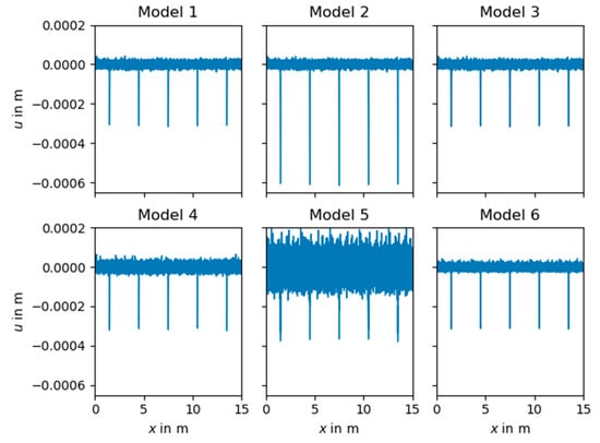
Figure 1.
Different synthetic data models according to Table 1.

Table 1.
Parameters of the different relative displacement models.
3.2. Cepstrum Analysis of Synthetic Data
A peak at a navewumber of 3 m can be noticed in the cepstra of all models (Figure 2). It indicates the wheel circumference. Comparing the cepstra of the first three models shows that with increasing wheel-flat depth the amplitude of this peak increases, while the length of the wheel flat has the opposite effect. A longer wheel flat is smoother or less spiky and the resulting harmonics in the spectrum are weaker, which leads to weaker peaks in the cepstrum. The cepstra of models 4 and 5 indicate that an increase in wheel roughness leads to an increase of the peak amplitude. However, comparing the cepstra of models 5 and 6 suggests that decreasing the amplitude of the rail roughness has a similar effect on the peak amplitude than increasing the amplitude of the wheel roughness. This can be explained by applying Equations (2)–(6) to Equation (7):
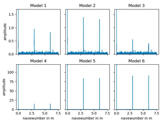
Figure 2.
Cepstra of the synthetic data generated of the different models.
The second term in Equation (11) shows that the power spectrum of the wheel profile is scaled by the power spectrum of the rail profile before the inverse Fourier transform is taken. Thus, the amplitude of the peak in the cepstrum at the wheel circumference can be interpreted as the relation between the contributions of the wheel and track to the relative displacement and hence to the dynamic wheel–rail interaction. If the rail roughness is zero, Equation (11) reduces to Equation (9) and the amplitudes of the wheel irregularities have no influence on the amplitude of the peaks at the wheel circumference.
4. Experimental Data
ABA data acquired during a measurement campaign in Austria were analyzed to investigate the performance of the cepstrum algorithm at normal operating conditions.
4.1. Data Acquisition
The data have been acquired with a prototype of a multi-sensor system developed at the German Aerospace Center (DLR, Institute of Transportation Systems, Braunschweig, Germany). The system comprises a GNSS receiver with external antenna, an inertial measurement unit and an analogue-to-digital converter with a three-axial analogue ABA sensor. The data acquisition and processing has been implemented in Robot Operating System (ROS). ABA data were recorded at a sampling rate of 20 kHz.
The system was installed on a measurement car of the Österreichische Bundesbahnen (ÖBB, Vienna, Austria, Figure 3). Data were gathered throughout a two-weeks measurement campaign in June 2019. During this campaign the measurement train was travelling at normal operating speed of up to 200 km/h.
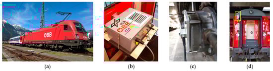
Figure 3.
(a) Measurement train; (b) Multi-sensor box inside the wagon; (c) Accelerometer mounted at the axle box; (d) Global navigation satellite system (GNSS) antenna (yellow box).
4.2. Speed Estimation and Data Pre-Processing
Speed information is essential in the presented ABA data analysis methodology and used to transform ABA time series into functions of a scalar along-track distance.
Speed information can be obtained from the GNSS and IMU signals. Both exhibit characteristic errors. GNSS reception is compromised in areas where the satellite sight is obstructed with, e.g., buildings or trees. Tunnels result in temporary signal outages. MEMS-IMU show slowly drifting bias errors. These shortcomings were accommodated in a sensor fusion framework with additional pre-processing steps to nevertheless obtain accurate speed information at a constant 100 Hz rate.
A simple Kalman filter (KF) [25] scheme was employed to fuse the speed information provided by the GNSS with the longitudinal IMU acceleration. Typical GNSS rates are around 1 Hz. Combination with the IMU data at around 100 Hz in a KF yields constant 100 Hz speed rates even during GNSS outages. The signal characteristics of both GNSS and IMU data depend on the vehicle state of motion. Therefore, a parallel motion and standstill detection scheme was implemented. For instance, vehicle standstill results in low instantaneous power of the IMU acceleration signals and can be detected accordingly. A viable option is to run a KF with a state vector comprising the scalar along-track velocity, acceleration and acceleration bias. Depending on the state of motion different KF time and measurement updates are performed iteratively. For instance, in standstill the speed and acceleration are known to be zero. Therefore, the bias can be observed in the noisy acceleration data. In motion one observes the sum of the acceleration and the bias. GNSS outlier removal can be performed by only using speed measurements with enough satellites in view. In addition to the state vector, the KF provides uncertainty information in the form of an estimation error covariance. The KF results were further improved offline in the following way: From the motion detection results the data can be divided into single sequences of motion, which we call journeys. For each journey the vehicle does not change direction. Hence, its velocity does not change its sign. With a Rauch–Tung–Striebel (RTS) smoother [25] the KF results of the individual journeys can be re-processed using an iteration that resembles a KF run backwards in time. The RTS iterations result in smoother state estimates and are especially beneficial in the presence of GNSS gaps.
The speed information is then used to separate the ABA time series into different journeys with a defined minimal speed. Furthermore, the speed is used to convert the data from time to distance domain. Subsequently, the data are resampled to an equidistant interval of 0.001 m. Notice, that at lower speed the data might be down-sampled, so that an anti-aliasing filter needs to be applied before resampling. Figure 4 depicts the track layout and Figure 5 shows the raw ABA together with the enhanced speed data from an 11 km journey with speeds between 10 m/s and 28 m/s.
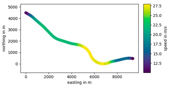
Figure 4.
GNSS train position and speed.
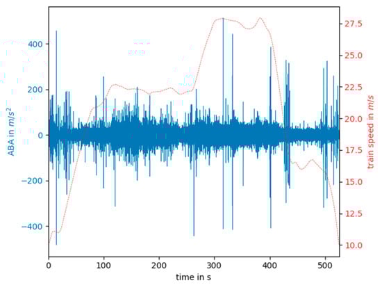
Figure 5.
Axle-box accelerations (ABA) data (solid blue line) and speed data (dashed red line) in the time domain.
4.3. Cepstrum Analysis of Experimental Data
The cepstrum analysis is performed for the data represented in Figure 5. First, the cepstrum was calculated for the whole length of the data (11,100 m). The cepstrum shows a distinct peak at a navewumber of 3 m that corresponds to the wheel circumference (Figure 6).
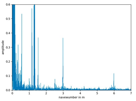
Figure 6.
Cepstrum of ABA data calculated from the whole journey with a length of 11,100 m.
In order to investigate the changes of the cepstrum along the train journey, the data was divided into segments of a certain length using a Hann window with 50% overlap. Then the cepstrum was calculated for each window and the peak position and amplitude determined between navewumbers of 2 m and 4 m. Different window sizes were tested. The results are shown in Table 2. For each test the median peak position across all windows was computed. Then, the percentage of windows in which the peak occurred in a range of 0.01 m around the median peak position and the mean amplitude of those peaks were determined. In Table 2, we refer to these peaks close to the median position as “correctly” depicted peaks. It can be seen that the median peak position is constant for all tests. The percentage of windows in which the peak position was close to the median position is very similar for windows larger than 20 m. It can be assumed that smaller windows are more affected by track singularities, which might mask the cepstral response of the wheel. The mean amplitude of the peaks of the shortest windows might be affected for the same reason.
Table 2.
Results of segmented cepstrum analysis with different window sizes.
The position of the cepstrum peaks and their amplitudes for segments of 40 m length are shown in Figure 7. The position of the cepstrum peak could be precisely recovered apart from a few locations. Especially at the beginning and the end of the journey, where the train speed is low, the algorithm struggles to find the right peak location. Therefore, we assume that a minimum speed of 15 m/s is necessary to provide reliable results.
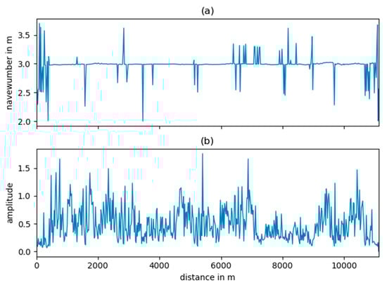
Figure 7.
Cepstrum analysis of 40-m-long track segments; (a) position of cepstrum peaks at navewumbers between two and four meters and (b) corresponding peak amplitude.
5. Discussion
5.1. Wheel Condition Monitoring with ABA Sensors
Wheel monitoring with train-borne sensors means that each wagon needs to be equipped with sensors. In contrast, wayside measurement systems are able to measure conditions of all wheelsets of each passing train with one measurement system. However, on-board systems provide a quasi-continuous monitoring of the wagon, while wayside systems only provide data in certain time intervals, when the train passes. Another advantage of train-borne measurement systems is that they can be used to monitor the track as well, which could justify the high number of sensors. Using broad-band accelerometers below the suspension, in contrast to sensors installed at the bogie or car body, allows to monitor the wheel diameter with very high resolution, which is beneficial for wheel-wear trend analysis. A comprehensive cost-benefit study of available wheel monitoring systems for condition-based and predictive maintenance was not part of this work but should be dealt with in future studies.
5.2. Navewumber Analysis
The navewumber analysis provides a robust tool to extract the wheel circumference from the ABA data. It can be recovered with a resolution equal to the distance between two measurement points, which depends on the train speed and sampling frequency. At a speed of 20 m/s and sampling frequency of 20 kHz the cepstral resolution is 0.001. We could show that between 80 and 90 percent of the calculated wheel circumferences were within a range of two millimeters along the whole train journey.
The high resolution and accuracy allow precise monitoring of the wheel diameter and therefore enable wheel-wear trend analysis. The approach provides reliable results under varying operational conditions. We found out that a minimal train speed of 15 m/s is sufficient to allow the estimation of the wheel circumference. Above this speed, the navewumber analysis is not affected by the train speed but its accuracy directly depends on the accuracy of the speed estimation that is used to transform the data from the time to distance domain. Thus, short-term variations of the estimated wheel diameter most likely relate to speed estimation errors. These Gaussian distributed errors can be estimated by the positioning algorithms introduced in Section 4.2.
It is especially noteworthy that the track condition only has a minor effect on the estimation of the wheel circumference. Even at track segments, where high wheel vibrations were excited, the wheel circumference could be determined accurately.
Due to the conicity of the wheels, the gauge and curve radius might have an influence on the estimated wheel circumference. However, the data analyzed in this study were not affected by the track geometry. Furthermore, the wear-related reduction of the wheel diameter is monotonic, while track-geometry changes only occur at certain track segments. Therefore, trend analysis of the wheel wear is not influenced by the track geometry. The influence of the track conditions can be further reduced by averaging over several track segments or taking longer track segments into account.
The synthetic data analysis has shown that the absolute amplitude of the cepstral peak can be similarly influenced by the track as well as wheel conditions. A mildly defected wheel running on a track with low roughness can produce a peak similar to that produced by a more severely defected wheel on a track with higher roughness. More generally, the amplitudes of the peaks in the navewumber domain provide a measure of the repeatability of the ABA signal and hence a measure of the relative contribution of the wheel condition to the dynamic wheel rail interaction.
The discrimination of different wheel defects using cepstral peak position and amplitude alone seems to be impracticable. Nevertheless, the cepstral features might complement other data driven approaches for wheel defect diagnosis.
It should be noticed that the measurement campaign, which builds the data base for this study did not focus on wheel monitoring but rather on testing the performance of the multi-sensor system. Therefore, no ground truth on the actual condition of the wheel exists. Nevertheless, no severe wheel defects were observed during operation. Hence, further tests including ground truth measurements and calibration by means of direct wheel profile measurements are required to determine thresholds for wheel defect detection. In principal, the methodology provided here, could be similarly used for the on-board detection of bearing defects, which should be subject of future studies.
6. Conclusions
The early detection of wheel defects is an important asset management and maintenance task. Wheel vibrations are excited by the imperfections of the wheel and rail and hence contain information on the health status of both assets. These vibrations can be measured by means of ABA sensors.
In this paper, a promising methodology, the cepstrum analysis, was tested for the application to wheel condition monitoring. The cepstrum is powerful in revealing periodic signals and separating them from the rest of the signal. This makes the cepstrum particularly interesting for wheel monitoring. The vibration signal excited by the wheel profile is periodic with respect to the wheel circumference. This periodicity changes with the rotational frequency of the wheel and hence depends on the speed of the train. This dependency can be compensated for by transforming the ABA data from the time to the spatial domain. To accomplish that, accurate speed information is necessary, which was obtained by fusing IMU and (E)GNSS data. The cepstral analysis was then performed in the spatial domain. The obtained cepstrum itself is then in a spatial domain, which we called navewumber domain to highlight the inverse relation to the wavenumber. The periodicity of the ABA signal excited by the wheel is then represented by a peak in the cepstrum at a wavenumber equal to the wheel circumference. The position of the peak precisely indicates the wheel circumference and can therefore be used to monitor the wheel diameter. The amplitude of this peak provides a measure of the relative contribution of the wheel to the combined wheel–rail roughness. The cepstral wheel monitoring approach presented here requires neither extensive hyperparameter testing nor training data. Ground truth data might be used to define hard thresholds for the detection of certain track defects. However, we think that it is more reasonable and also sufficient to monitor changes in the cepstral features and thus detect deviations from the normal behavior that can be related to wheel defects.
Through the analysis of experimental data, we could show that the cepstrum analysis is robust under varying operating conditions.
From these findings we conclude that cepstral analysis of ABA data is a powerful methodology to monitor the wear-related reduction of the wheel circumference and to detect and monitor the evolution of wheel surface defects.
Author Contributions
Conceptualization, B.B.; methodology, B.B.; software, B.B., J.H., T.N. and M.R.; validation, B.B., J.H. and T.N.; formal analysis, T.N.; investigation, B.B.; data curation, J.H.; writing—original draft preparation, B.B.; writing—review and editing, J.H. and M.R.; visualization, B.B.; supervision, B.B.; project administration, M.R. All authors have read and agreed to the published version of the manuscript.
Funding
This project has received funding from the European GNSS Agency under the European Union’s Horizon 2020 research and innovation program under grant agreement No. 776402.
Institutional Review Board Statement
Not applicable.
Informed Consent Statement
Not applicable.
Data Availability Statement
Restrictions apply to the availability of these data. Data was obtained in collaboration with the Österreichische Bundesbahnen (ÖBB, Vienna, Austria) and are available on request from the corresponding author only with permission of the ÖBB.
Acknowledgments
We would like to thank the ÖBB for providing the measurement train and for guidance and support during the measurement campaign. We would like to thank the two anonymous reviewers for their valuable comments and advice, which helped to improve the manuscript.
Conflicts of Interest
The authors declare no conflict of interest.
References
- Krummenacher, G.; Ong, C.S.; Koller, S.; Kobayashi, S.; Buhmann, J.M. Wheel Defect Detection with Machine Learning. IEEE Trans. Intell. Transport. Syst. 2018, 19, 1176–1187. [Google Scholar] [CrossRef]
- Nielsen, J.C.O.; Johansson, A. Out-of-round railway wheels—A literature survey. Proc. Inst. Mech. Eng. Part F J. Rail Rapid Transit 2000, 214, 79–91. [Google Scholar] [CrossRef]
- Bian, J.; Gu, Y.; Murray, M.H. A dynamic wheel-rail impact analysis of railway track under wheel flat by finite element analysis. Veh. Syst. Dyn. 2013, 51, 784–797. [Google Scholar] [CrossRef]
- Bogacz, R.; Frischmuth, K. On dynamic effects of wheel-rail interaction in the case of Polygonalisation. Mech. Syst. Signal Process. 2016, 79, 166–173. [Google Scholar] [CrossRef]
- Telliskivi, T.; Olofsson, U. Wheel-rail wear simulation. Wear 2004, 257, 1145–1153. [Google Scholar] [CrossRef]
- Casanueva, C.; Enblom, R.; Stichel, S.; Berg, M. On integrated wheel and track damage prediction using vehicle–track dynamic simulations. Proc. Inst. Mech. Eng. Part F J. Rail Rapid Transit 2017, 231, 775–785. [Google Scholar] [CrossRef]
- Mosleh, A.; Montenegro, P.; Alves Costa, P.; Calçada, R. An approach for wheel flat detection of railway train wheels using envelope spectrum analysis. Struct. Infrastruct. Eng. 2020, 202, 1–20. [Google Scholar] [CrossRef]
- Molodova, M.; Li, Z.; Dollevoet, R. Axle box acceleration: Measurement and simulation for detection of short track defects. Wear 2011, 271, 349–356. [Google Scholar] [CrossRef]
- Mori, H.; Sato, Y.; Ohno, H.; Tsunashima, H.; Saito, Y. Development of Compact Size Onboard Device for Condition Monitoring of Railway Tracks. J. Mech. Syst. Transp. Logist. 2013, 6, 142–149. [Google Scholar] [CrossRef][Green Version]
- Lederman, G.; Chen, S.; Garrett, J.; Kovačević, J.; Noh, H.Y.; Bielak, J. Track-monitoring from the dynamic response of an operational train. Mech. Syst. Signal Process. 2017, 87, 1–16. [Google Scholar] [CrossRef]
- Baasch, B.; Roth, M.; Groos, J. In-service condition monitoring of rail tracks: On an on-board low-cost multi-sensor system for condition based maintenance of railway tracks. Int. Verk. 2018, 70, 76–79. [Google Scholar]
- Niebling, J.; Baasch, B.; Kruspe, A. Analysis of Railway Track Irregularities with Convolutional Autoencoders and Clustering Algorithms. In Dependable Computing—EDCC 2020 Workshops; Bernardi, S., Vittorini, V., Flammini, F., Nardone, R., Marrone, S., Adler, R., Schneider, D., Schleiß, P., Nostro, N., Løvenstein Olsen, R., Eds.; Springer International Publishing: Cham, Switzerland, 2020; pp. 78–89. [Google Scholar]
- Li, C.; Luo, S.; Cole, C.; Spiryagin, M. An overview: Modern techniques for railway vehicle on-board health monitoring systems. Veh. Syst. Dyn. 2017, 55, 1045–1070. [Google Scholar] [CrossRef]
- Bosso, N.; Gugliotta, A.; Zampieri, N. Wheel flat detection algorithm for onboard diagnostic. Measurement 2018, 123, 193–202. [Google Scholar] [CrossRef]
- Heirich, O.; Steingass, A.; Lehner, A.; Strang, T. Velocity and location information from onboard vibration measurements of rail vehicles. In Proceedings of the 16th International Conference on Information Fusion, Istanbul, Turkey, 9–12 July 2013; pp. 1835–1840. [Google Scholar]
- Jia, S.; Dhanasekar, M. Detection of Rail Wheel Flats using Wavelet Approaches. Struct. Health Monit. 2016, 6, 121–131. [Google Scholar] [CrossRef]
- Ye, Y.; Shi, D.; Krause, P.; Hecht, M. A data-driven method for estimating wheel flat length. Veh. Syst. Dyn. 2019, 213, 1–19. [Google Scholar] [CrossRef]
- Bai, Y.; Yang, J.; Wang, J.; Li, Q. Intelligent Diagnosis for Railway Wheel Flat Using Frequency-Domain Gramian Angular Field and Transfer Learning Network. IEEE Access 2020, 8, 105118–105126. [Google Scholar] [CrossRef]
- Childers, D.G.; Skinner, D.P.; Kemerait, R.C. The cepstrum: A guide to processing. Proc. IEEE 1977, 65, 1428–1443. [Google Scholar] [CrossRef]
- Oppenheim, A.V.; Schafer, R.W. From frequency to quefrency: A history of the cepstrum. IEEE Signal Process. Mag. 2004, 21, 95–106. [Google Scholar] [CrossRef]
- Bogert, B.P.; Healy, M.J.; Tukey, J.W. The quefrency alanysis of time series for echoes: Cepstrum, pseudo-autocovariance, cross-cepstrum, and saphe cracking. In Proceedings of the Symposium on Time Series Analysis, Brown-University, Providence, RI, USA, 11–14 June 1962; John Wiley & Sons: New York, NY, USA; London, UK, 1963; pp. 209–243. [Google Scholar]
- Bracciali, A.; Cascini, G. Detection of corrugation and wheelflats of railway wheels using energy and cepstrum analysis of rail acceleration. Proc. Inst. Mech. Eng. Part F J. Rail Rapid Transit 1997, 211, 109–116. [Google Scholar] [CrossRef]
- Teunissen, P.J.; Montenbruck, O. (Eds.) Springer Handbook of Global Navigation Satellite Systems; Springer International Publishing: Cham, Switzerland, 2017. [Google Scholar]
- Groves, P.D. Principles of GNSS, Inertial, and Multisensor Integrated Navigation Systems, 2nd ed.; Artech House: Boston, MA, USA, 2013. [Google Scholar]
- Gustafsson, F. Statistical Sensor Fusion; Studentlitteratur: Lund, Sweden, 2010. [Google Scholar]
- Buttkus, B. Homomorphic Filtering—Theory and Practice. Geophys. Prospect. 1975, 23, 712–748. [Google Scholar] [CrossRef]
- Ulrych, T.J. Application of homomorphic deconvolution to seismology. Geophysics 1971, 36, 650–660. [Google Scholar] [CrossRef]
- Wu, T.; Thompson, D. Theoretical Investigation of Wheel/Rail Non-Linear Interaction due to Roughness Excitation. Veh. Syst. Dyn. 2000, 34, 261–282. [Google Scholar] [CrossRef]
Publisher’s Note: MDPI stays neutral with regard to jurisdictional claims in published maps and institutional affiliations. |
© 2021 by the authors. Licensee MDPI, Basel, Switzerland. This article is an open access article distributed under the terms and conditions of the Creative Commons Attribution (CC BY) license (http://creativecommons.org/licenses/by/4.0/).