
Prediction of Wide Range Two-Dimensional Refractivity Using an IDW Interpolation Method from High-Altitude Refractivity Data of Multiple Meteorological Observatories


Abstract
1. Introduction
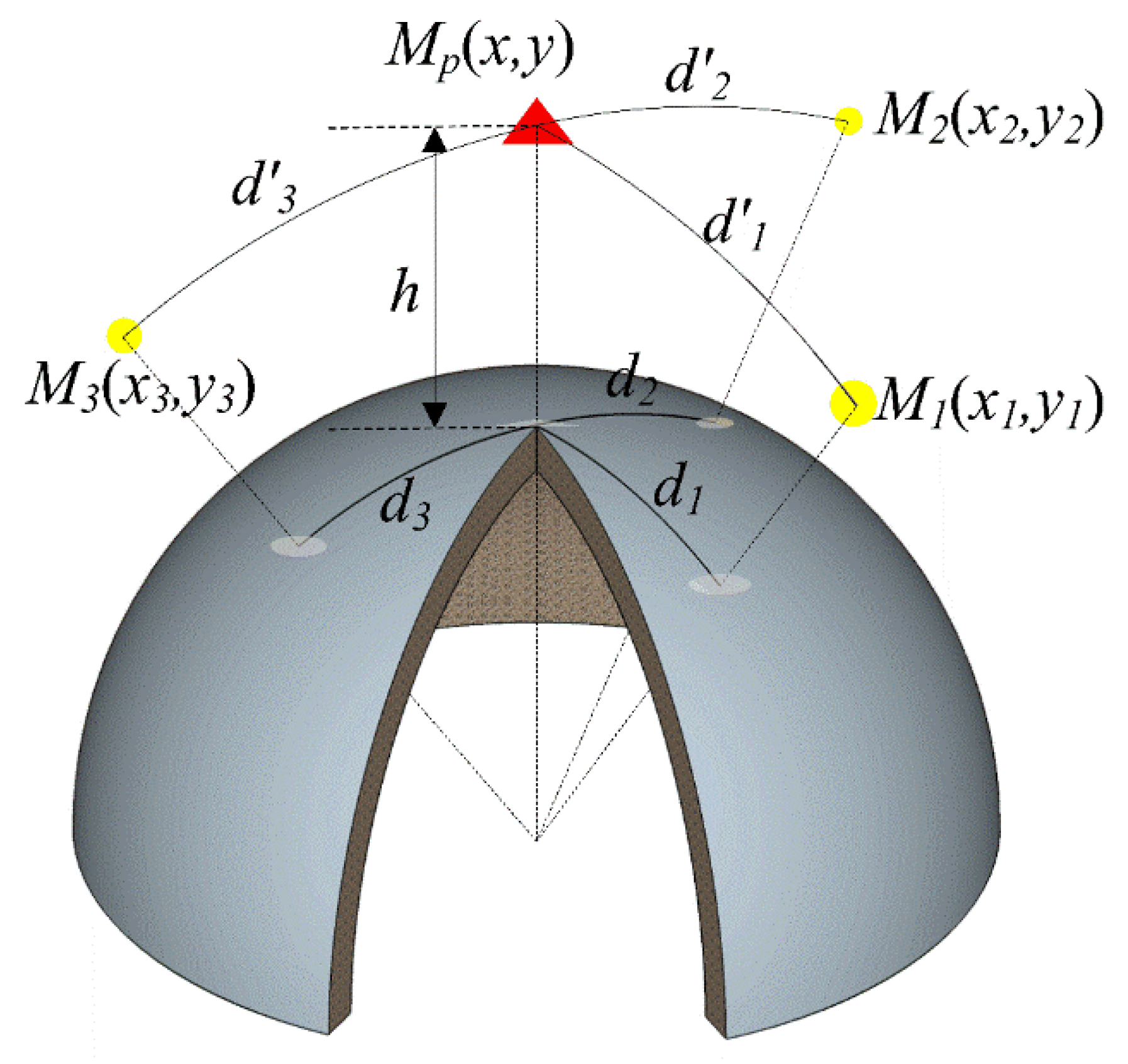
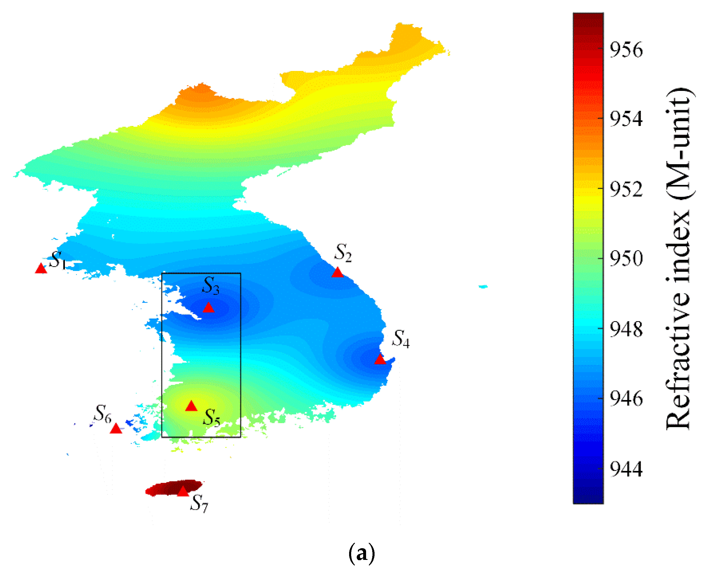
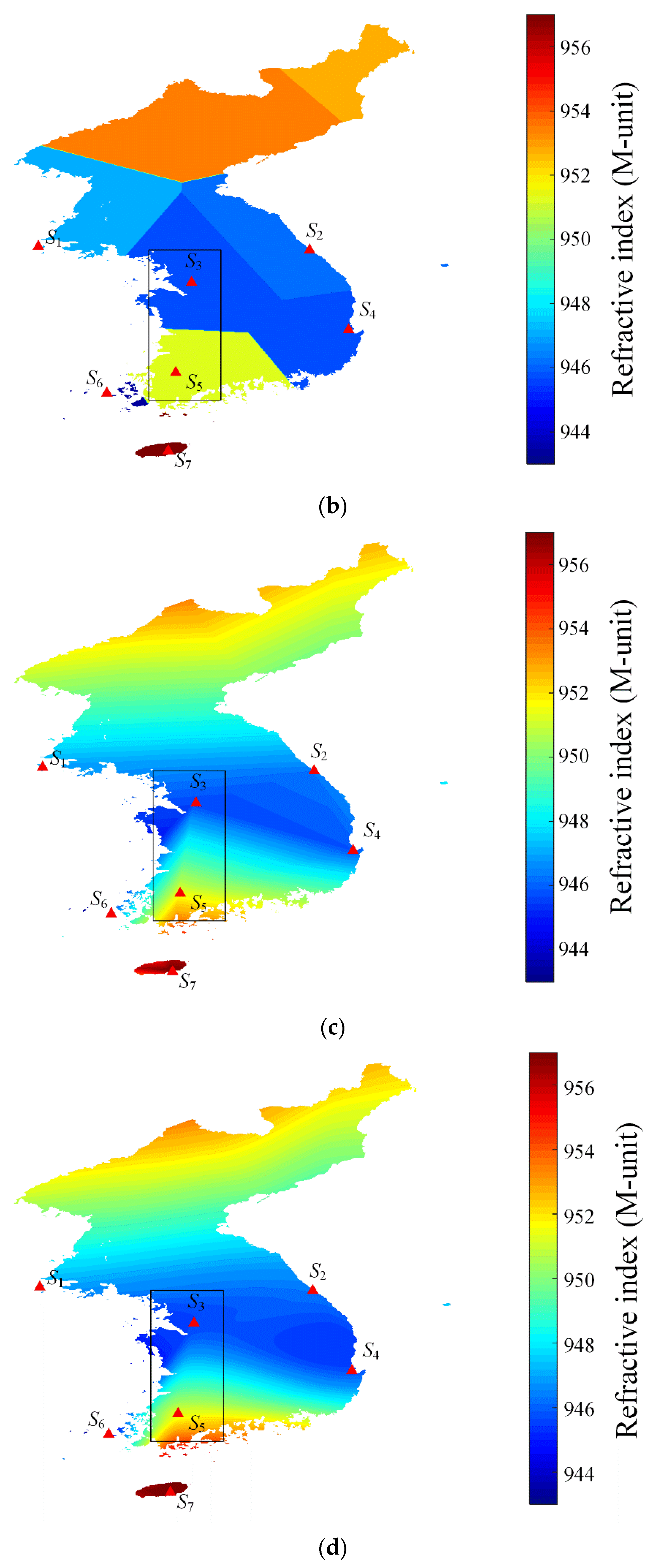
2. Wide Range Two-Dimensional High-Altitude Refractivity Estimation
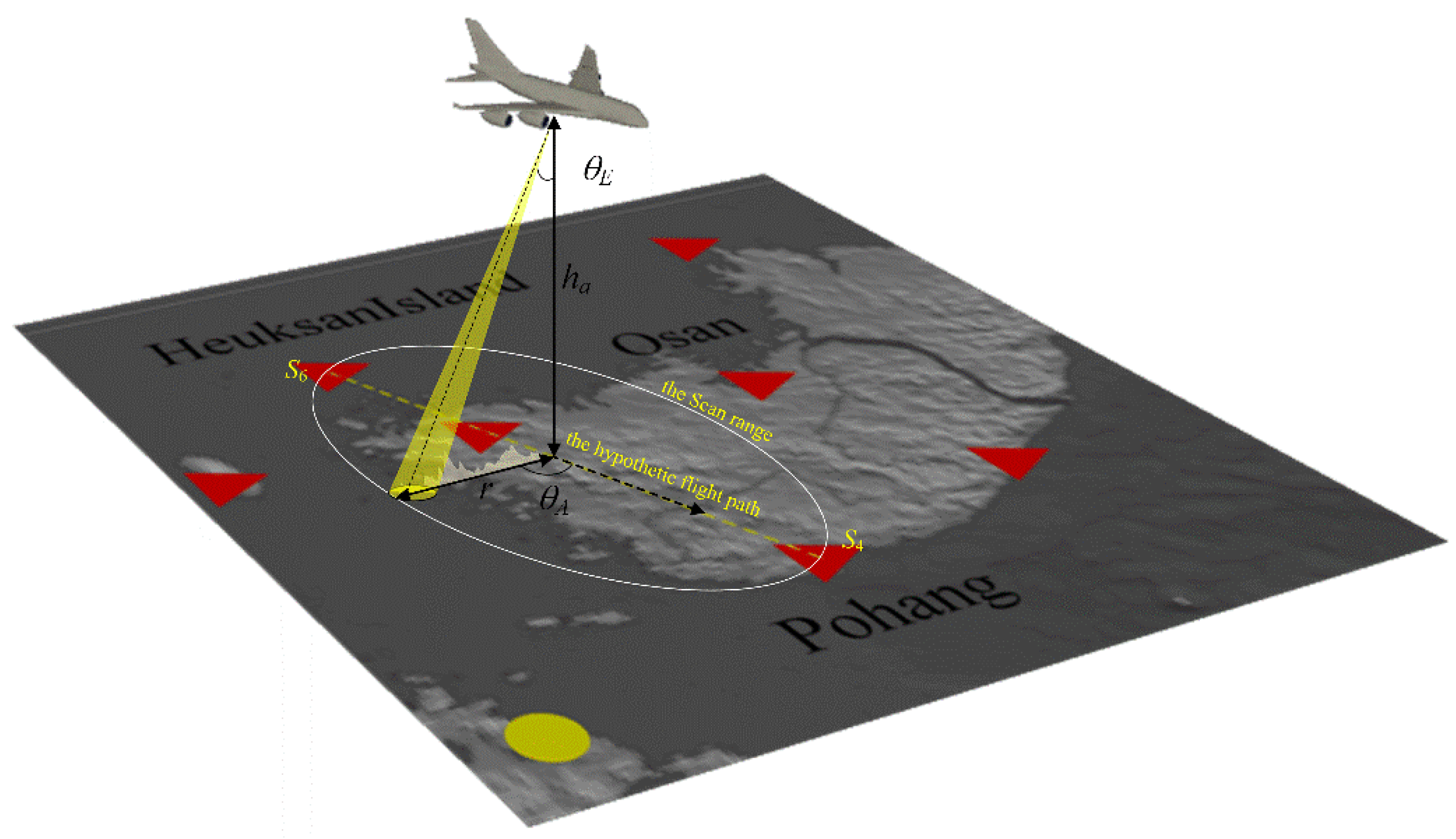
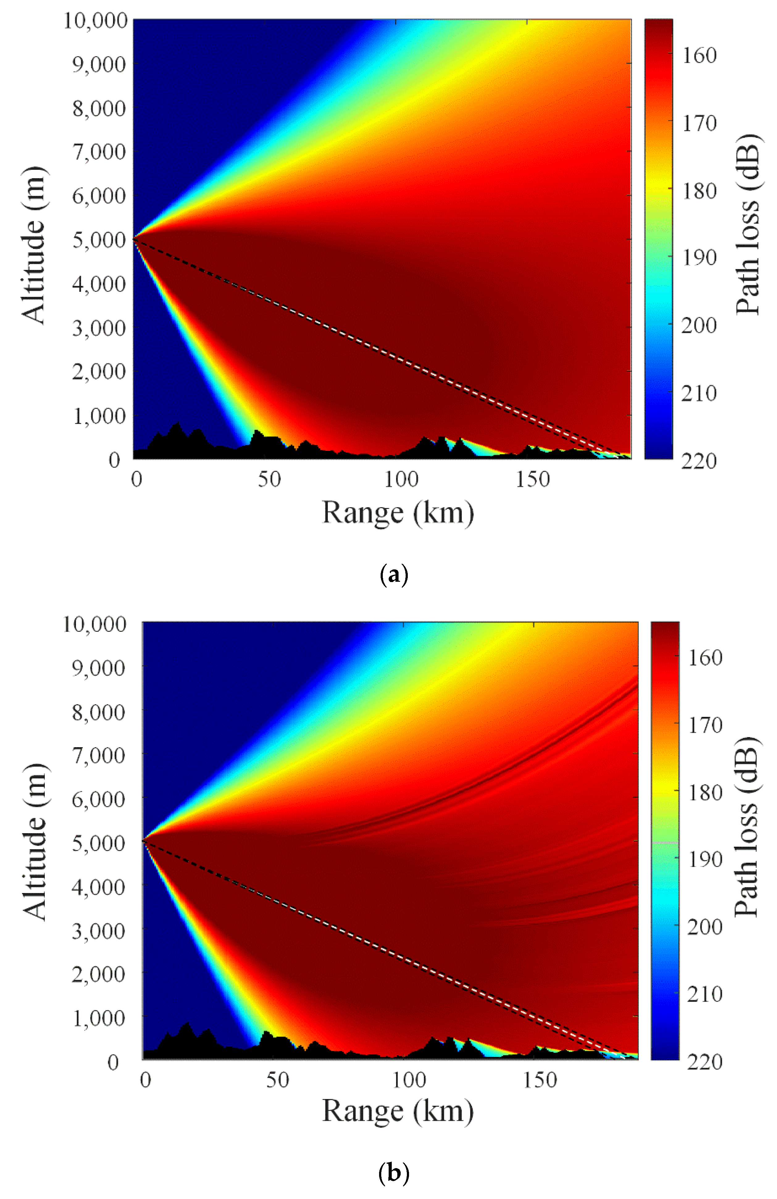
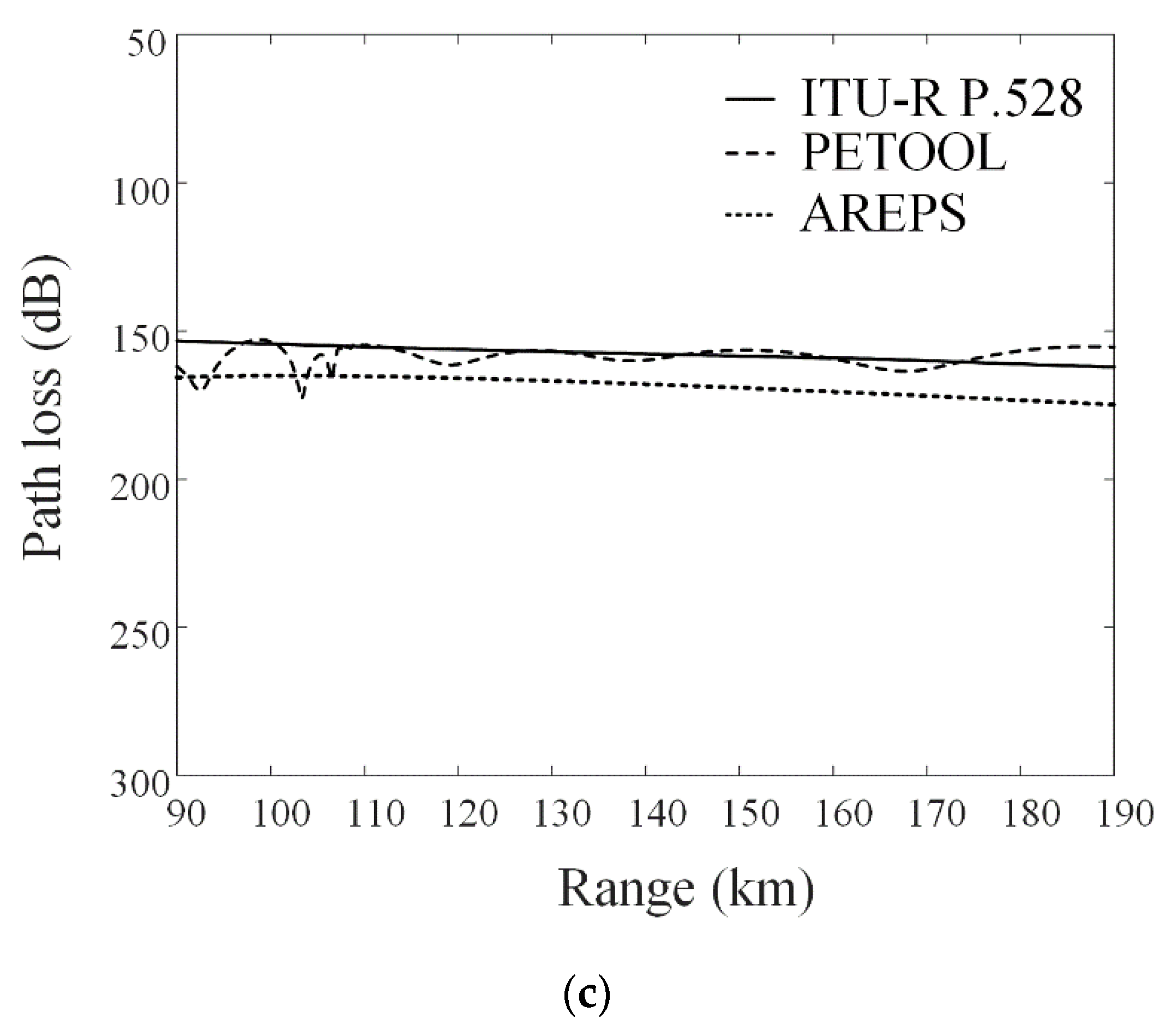
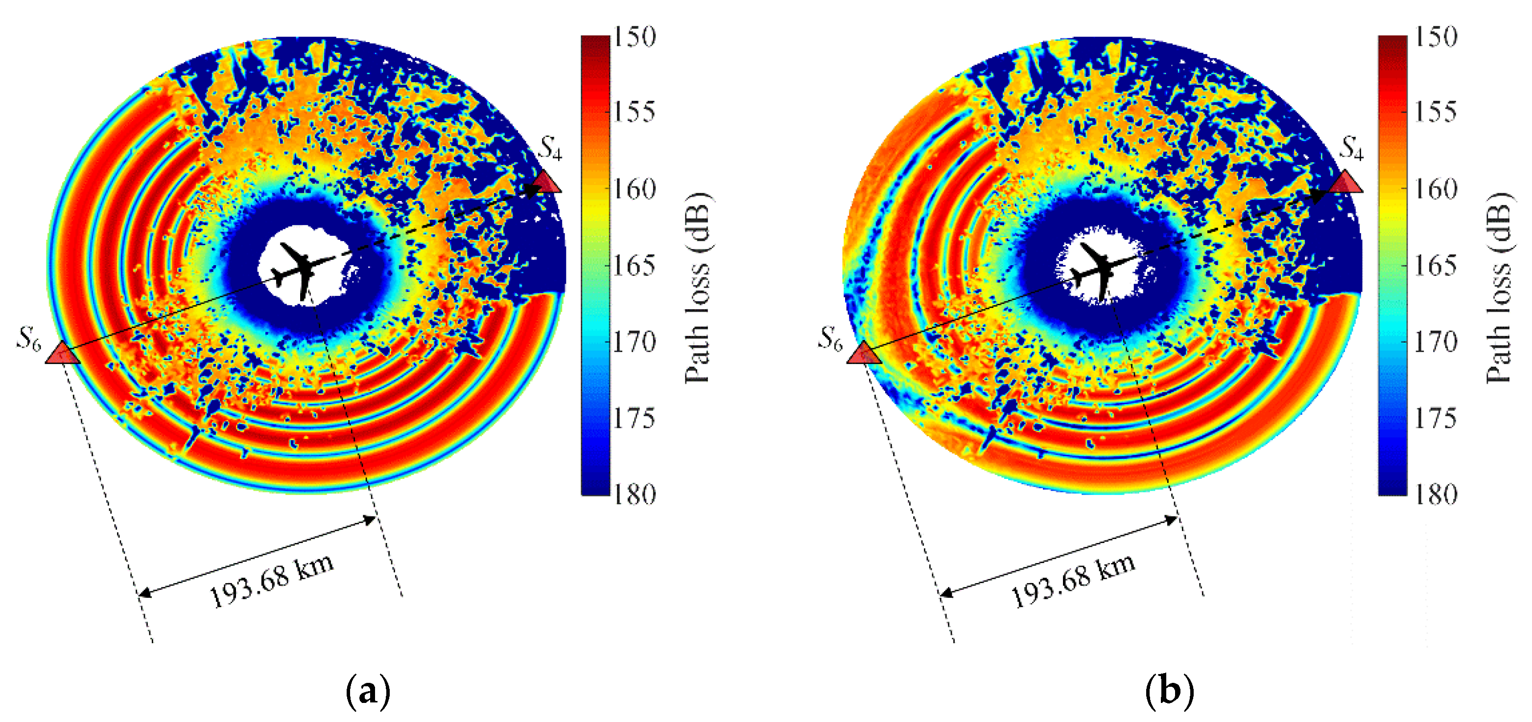
3. Path Loss Simulation and Illuminated Field Intensity Observation in an Air-to-Ground Scenario
4. Conclusions
Author Contributions
Funding
Institutional Review Board Statement
Informed Consent Statement
Data Availability Statement
Conflicts of Interest
References
- Lim, S.; Choi, I.; Jeong, T. Compensation method for a wideband signal’s squint problem of an AESA SAR system using a cross-range-variant antenna gain equalizer. IEEE Sens. J. 2019, 19, 2937–2945. [Google Scholar] [CrossRef]
- Frey, O.; Magnard, C.; Ruegg, M.; Meier, E. Focusing of airborne synthetic aperture radar data from highly nonlinear flight tracks. IEEE Trans. Geosci. Remote Sens. 2009, 47, 1844–1858. [Google Scholar] [CrossRef]
- Kim, C.K.; Lee, J.S.; Chae, J.S.; Park, S.O. A modified stripmap SAR processing for vector velocity compensation using the cross-correlation estimation method. J. Electromagn. Eng. Sci. 2019, 19, 159–165. [Google Scholar] [CrossRef]
- Stailey, J.E.; Hondl, K.D. Multifunction phased array radar for aircraft and weather surveillance. Proc. IEEE 2016, 104, 649–659. [Google Scholar] [CrossRef]
- Barfield, A.F.; Probert, J.; Browning, D. All terrain ground collision avoidance and maneuvering terrain following for automated low level night attack. IEEE Aerosp. Electron. Syst. Mag. 1993, 8, 40–47. [Google Scholar] [CrossRef]
- Dickey, F.R.; Labitt, M.; Staudaher, F.M. Development of airborne moving target radar for long range surveillance. IEEE Trans. Aerosp. Electron. Syst. 1991, 27, 959–972. [Google Scholar] [CrossRef]
- Kim, E.; Park, J.Y. Dwell time optimization of alert-confirm detection for active phased array radars. J. Electromagn. Eng. Sci. 2019, 19, 107–114. [Google Scholar] [CrossRef]
- Du, Y.; Jiang, Y.; Wang, Y.; Zhou, W.; Liu, Z. ISAR Imaging for low-earth-orbit target based on coherent integrated smoothed generalized cubic phase function. IEEE Trans. Geosci. Remote Sens. 2020, 58, 1205–1220. [Google Scholar] [CrossRef]
- Xu, G.; Xing, M.; Xia, X.; Chen, Q.; Zhang, L.; Bao, Z. High-resolution inverse synthetic aperture radar imaging and scaling with sparse aperture. IEEE J. Sel. Top. Appl. Earth Observ. Remote Sens. 2015, 8, 4010–4027. [Google Scholar] [CrossRef]
- Rémy, D.; Bonvalot, S.; Briole, P.; Murakami, M. Accurate measurements of tropospheric effects in volcanic areas from SAR interferometry data: Application to Sakurajima volcano (Japan). Earth Planet. Sci. Lett. 2003, 213, 299–310. [Google Scholar] [CrossRef]
- Sun, J.; Bi, Y.; Wang, Y.; Hong, W. High resolution SAR performance limitation by the change of tropospheric refractivity. In Proceedings of the 2011 IEEE CIE International Conference on Radar, Chengdu, China, 24–27 October 2011; pp. 1448–1451. [Google Scholar]
- Valtr, P.; Pechac, P. The influence of horizontally variable refractive index height profile on radio horizon range. IEEE Antennas Wirel. Propag. Lett. 2005, 4, 489–491. [Google Scholar] [CrossRef]
- Karimian, A.; Yardim, C.; Gerstoft, P.; Hodgkiss, W.S.; Barrios, A.E. Refractivity estimation from sea clutter: An invited review. Radio Sci. 2011, 46, 1–16. [Google Scholar] [CrossRef]
- Wagner, M.; Gerstoft, P.; Rogers, T. Estimating refractivity from propagation loss in turbulent media. Radio Sci. 2016, 51, 1876–1894. [Google Scholar] [CrossRef]
- James, R.; James, H.; Roger, S. Environmental/Noise Effects on VHF/UHF UWB SAR; Institute for Defense Analyses: Alexandria, VA, USA, 1998. [Google Scholar]
- Vasilescu, G. External Noise. In Electronic Noise and Interfering Signals; Signals and Communication Technology; Springer: Berlin/Heidelberg, Germany, 2005; pp. 255–257. [Google Scholar]
- Wang, L.; Wei, M.; Yang, T.; Liu, P. Effects of atmospheric refraction on an airborne weather radar detection and correction method. Adv. Meteorol. 2015, 2015, 407867. [Google Scholar] [CrossRef]
- Radiocommunication sector of ITU. Recommendation ITU-R P.453-13: The Radio Refractive Index: Its Formula and Refractivity Data; International Telecommunication Union: Geneva, Switzerland, 2017. [Google Scholar]
- Dinc, E.; Akan, O.B. Channel model for the surface ducts: Largescale path-loss, delay spread, and AOA. IEEE Trans. Antennas Propag. 2015, 63, 2728–2738. [Google Scholar] [CrossRef]
- Qixiang, L.; Zheng, S.; Hanqing, S.; Jie, X.; Hong, Y. Estimation of surface duct using ground-based GPS phase delay and propagation loss. Remote Sens. 2018, 10, 724. [Google Scholar]
- Julian, C.; Oscar, B.; Ono, A. Evaluation of EM-wave propagation in fully three-dimensional atmospheric refractive index distributions. Radio Sci. 2009, 44, 1–19. [Google Scholar]
- Lin, L.K.; Zhao, Z.W.; Zhang, Y.R.; Zhu, Q.L. Tropospheric refractivity profiling based on refractivity profile model using single ground-based global positioning system. IET Radar Sonar Navig. 2011, 5, 7–11. [Google Scholar] [CrossRef]
- Abdulhadi, A.; Raed, A.A.A.; Steve, M.R.J.; Hussain, A.A. New methodology for predicting vertical atmospheric profile and propagation parameters in subtropical Arabian Gulf Region. IEEE Trans. Antennas Propag. 2015, 63, 4057–4068. [Google Scholar]
- Shi, Y.; Yang, K.D.; Yang, Y.X.; Ma, Y.L. Experimental verification of effect of horizontal inhomogeneity of evaporation duct on electromagnetic wave propagation. Chin. Phys. B 2015, 24, 044102. [Google Scholar] [CrossRef]
- Pozderac, J.; Johnson, J.; Yardim, C.; Merrill, C.; de Paolo, T.; Terrill, E.; Ryan, F.; Frederickson, P. X-band beacon-receiver array evaporation duct height estimation. IEEE Trans. Antennas Propag. 2018, 66, 2545–2556. [Google Scholar] [CrossRef]
- Norman, R.J.; Marshall, J.L.; Rohm, W.; Carter, B.A.; Kirchengast, G.; Alexander, S.; Liu, C.; Zhang, K. Simulating the impact of refractive transverse gradients resulting from a severe troposphere weather event on GPS signal propagation. IEEE J. Sel. Top. Appl. Earth Observ. Remote Sens. 2015, 8, 418–424. [Google Scholar] [CrossRef]
- University of Wyoming, Department of Atmospheric Science. Available online: https://weather.uwyo.edu/upperair/sounding.html (accessed on 31 January 2020).
- National Geographic Information Institute. Available online: https://www.ngii.go.kr/kor/main.do (accessed on 31 January 2020).
- A MATLAB-based One-Way and Two-Way Split-Step Parabolic Equation Software Tool (PETOOL). Available online: http://cpc.cs.qub.ac.uk/summaries/AEJS_v1_0.html (accessed on 30 August 2018).
- Martin, G.; Pavel, P.; Pavel, V. On horizontal distribution of vertical gradient of atmospheric refractivity: Horizontal distribution of vertical gradient of atmospheric refractivity. Atmos. Sci. Lett. 2017, 18, 294–299. [Google Scholar]
- Advanced Refractive Prediction System (AREPS); Ver. 3.6; The Space and Naval Warfare System: San Diego, CA, USA, 2005.
- Radiocommunication sector of ITU. Recommendation ITU-R P.528-4: A Propagation Prediction Method for Aeronautical Mobile and Radionavigation Services Using the VHF, UHF and SHF Bands; International Telecommunication Union: Geneva, Switzerland, 2019. [Google Scholar]
- Balanis, C.A. Antenna Theory; John Wiley & Sons, Inc.: Hoboken, NJ, USA, 2005; ISBN 0-471-66782-X. [Google Scholar]


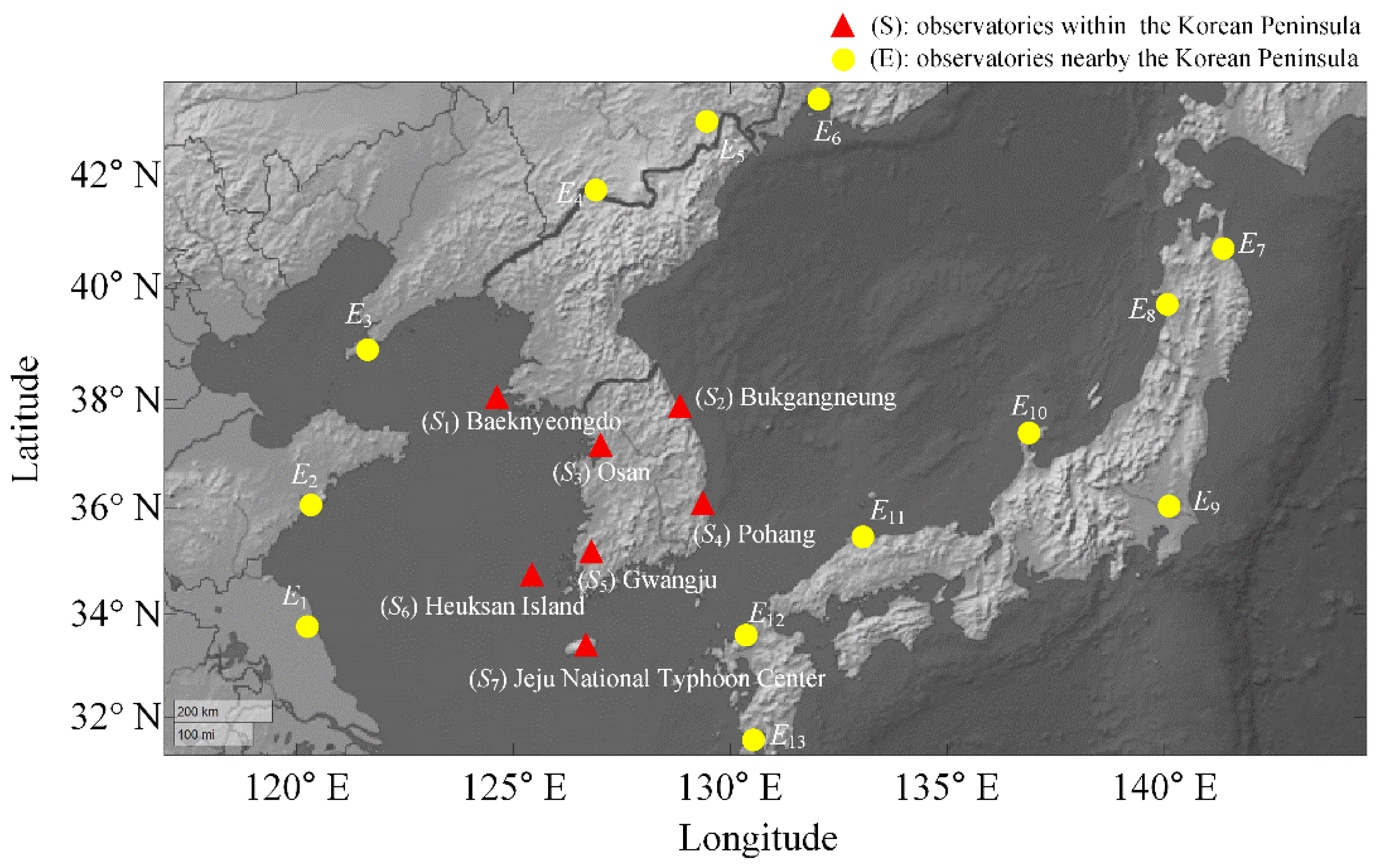
| Site | Meteorological Observatory | Latitude | Longitude | Height | Average Altitude Interval | Number of Measurements per Day |
|---|---|---|---|---|---|---|
| S1 | Baeknyeongdo | 37.97 | 124.63 | 158 m | 315.3 m | 2 |
| S2 | Bukgangneung | 37.81 | 128.85 | 89 m | 303.1 m | 2 |
| S3 | Osan | 37.10 | 127.03 | 52 m | 310.8 m | 4 |
| S4 | Pohang | 36.03 | 129.38 | 6 m | 308.7 m | 2 |
| S5 | Gwangju | 35.11 | 126.81 | 13 m | 308.5 m | 4 |
| S6 | Heuksando | 34.68 | 125.45 | 69 m | 293.3 m | 2 |
| S7 | Jeju National Typhoon Center | 33.33 | 126.68 | 235 m | 296.8 m | 2 |
| E1 | Sheyang | 33.76 | 120.25 | 7 m | 750.3 m | 2 |
| E2 | Qingdao | 36.06 | 120.33 | 77 m | 746.7 m | 2 |
| E3 | Dalian | 38.90 | 121.63 | 97 m | 1284.8 m | 2 |
| E4 | Jakangdo | 41.71 | 126.91 | 333 m | 1318.4 m | 2 |
| E5 | Yanbian | 42.88 | 129.46 | 178 m | 1319.0 m | 2 |
| E6 | Vladivostok | 43.26 | 132.05 | 82 m | 306.2 m | 2 |
| E7 | Misawa | 40.70 | 141.38 | 39 m | 399.5 m | 2 |
| E8 | Akita | 39.71 | 140.10 | 7 m | 345.1 m | 2 |
| E9 | Tateno | 36.05 | 140.13 | 31 m | 326.6 m | 2 |
| E10 | Wajima | 37.38 | 136.90 | 14 m | 291.7 m | 2 |
| E11 | Matsue | 35.45 | 133.07 | 22 m | 290.4 m | 2 |
| E12 | Fukuoka | 33.58 | 130.38 | 15 m | 322.2 m | 2 |
| E13 | Kagoshima | 31.55 | 130.55 | 31 m | 319.5 m | 2 |
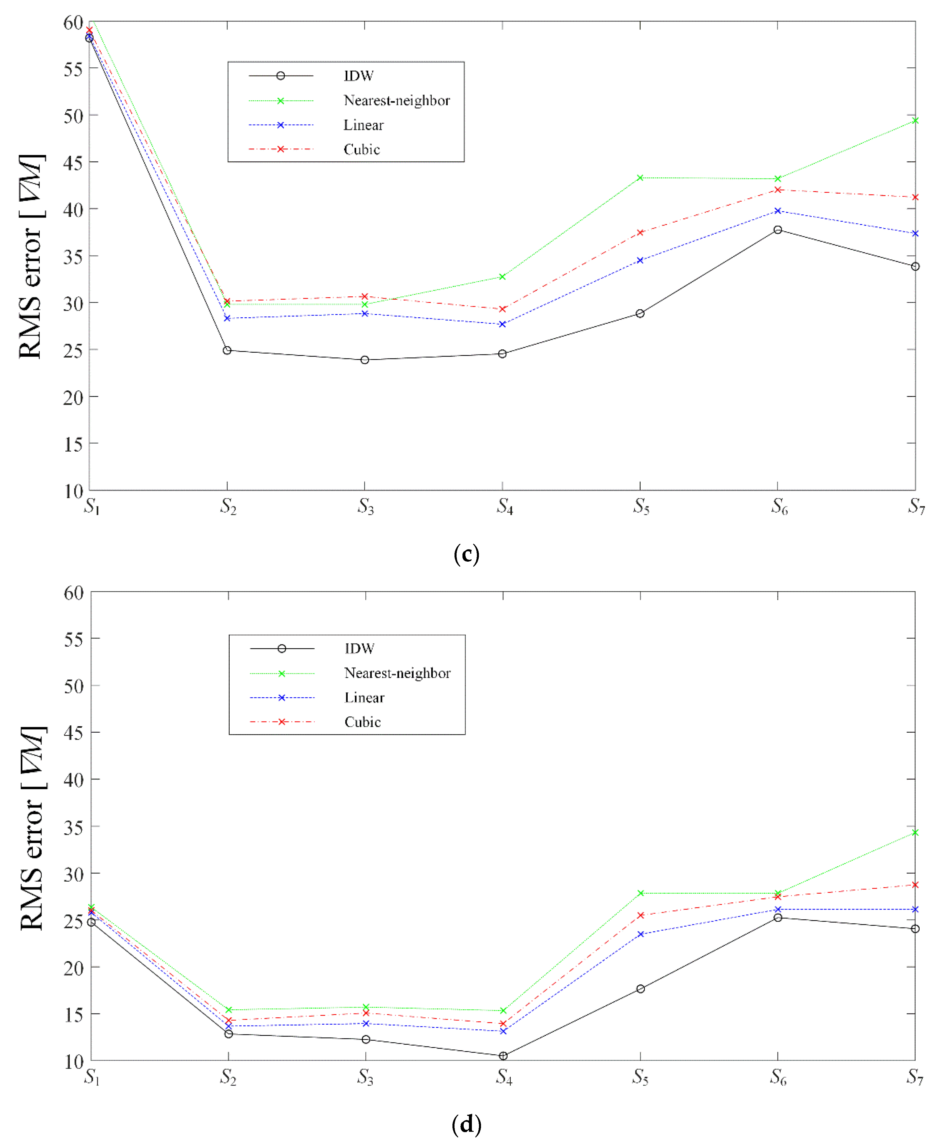
| Site | Meteorological Observatory | IDW (0 m/5000 m/Avg) | Linear (0 m/5000 m/Avg) | Cubic (0 m/5000 m/Avg) | Nearest (0 m/5000 m/Avg) |
|---|---|---|---|---|---|
| S1 | Baeknyeongdo | 62.6/30.0/31.1 | 64.3/29.0/30.0 | 64.1/29.3/30.3 | 65.0/29.5/33.2 |
| S2 | Bukgangneung | 20.1/27.7/27.8 | 18.4/38.5/34.0 | 18.7/42.4/36.5 | 24.5/26.0/29.6 |
| S3 | Osan | 18.3/12.0/17.6 | 24.9/16.1/19.8 | 26.6/18.6/21.7 | 24.4/26.0/29.6 |
| S4 | Pohang | 11.4/41.9/34.5 | 13.2/43.6/36.3 | 14.6/44.6/37.2 | 18.7/48.3/41.1 |
| S5 | Gwangju | 14.4/34.9/31.1 | 17.3/44.7/38.5 | 19.2/49.0/42.3 | 25.1/58.1/51.3 |
| S6 | Heuksando | 22.4/52.1/46.6 | 22.2/54.3/48.0 | 23.2/55.9/49.2 | 24.5/58.2/51.4 |
| S7 | Jeju National Typhoon Center | 30.0/56.7/55.0 | 31.0/57.7/55.4 | 32.3/61.0/57.6 | 34.8/69.7/65.6 |
| Parameters | Values |
|---|---|
| Altitude of the airborne transmitter (ha) | 5000 m |
| Scanning range (2r) | 387.4 km |
| Angle between flight direction and main beam direction (θA) | 0~360° |
| Beam pattern | Gaussian |
| Beam width | 2° |
| Steering angle (θE) | 2° |
| Polarization | Vertical |
| Tx frequency | 10 GHz |
Publisher’s Note: MDPI stays neutral with regard to jurisdictional claims in published maps and institutional affiliations. |
© 2021 by the authors. Licensee MDPI, Basel, Switzerland. This article is an open access article distributed under the terms and conditions of the Creative Commons Attribution (CC BY) license (http://creativecommons.org/licenses/by/4.0/).
Share and Cite
Wang, S.; Lim, T.H.; Oh, K.; Seo, C.; Choo, H. Prediction of Wide Range Two-Dimensional Refractivity Using an IDW Interpolation Method from High-Altitude Refractivity Data of Multiple Meteorological Observatories. Appl. Sci. 2021, 11, 1431. https://doi.org/10.3390/app11041431
Wang S, Lim TH, Oh K, Seo C, Choo H. Prediction of Wide Range Two-Dimensional Refractivity Using an IDW Interpolation Method from High-Altitude Refractivity Data of Multiple Meteorological Observatories. Applied Sciences. 2021; 11(4):1431. https://doi.org/10.3390/app11041431
Chicago/Turabian StyleWang, Sungsik, Tae Heung Lim, Kyoungsoo Oh, Chulhun Seo, and Hosung Choo. 2021. "Prediction of Wide Range Two-Dimensional Refractivity Using an IDW Interpolation Method from High-Altitude Refractivity Data of Multiple Meteorological Observatories" Applied Sciences 11, no. 4: 1431. https://doi.org/10.3390/app11041431
APA StyleWang, S., Lim, T. H., Oh, K., Seo, C., & Choo, H. (2021). Prediction of Wide Range Two-Dimensional Refractivity Using an IDW Interpolation Method from High-Altitude Refractivity Data of Multiple Meteorological Observatories. Applied Sciences, 11(4), 1431. https://doi.org/10.3390/app11041431