Article

Viscoelastic Model and Synthetic Seismic Data of Eastern Rub’Al-Khali

by
Septriandi A. Chan
1,†,
Paul Edigbue
1,†,
Sikandar Khan
2,†,
Abdul L. Ashadi
1,† and
Abdullatif A. Al-Shuhail
1,*,†
1
Geosciences Department, King Fahd University of Petroleum & Minerals, Dhahran 34464, Saudi Arabia
2
Mechanical Engineering Department, King Fahd University of Petroleum & Minerals, Dhahran 34464, Saudi Arabia
*
Author to whom correspondence should be addressed.
These authors contributed equally to this work.
Appl. Sci. 2021, 11(4), 1401; https://doi.org/10.3390/app11041401
Submission received: 4 December 2020 / Revised: 21 January 2021 / Accepted: 26 January 2021 / Published: 4 February 2021
(This article belongs to the Special Issue Advances in Applied Geophysics)

Abstract

:
The Rub’ Al-Khali basin in Saudi Arabia remains unexplored and lacks data availability due to its remoteness and the challenging nature of its terrain. Thus far, there are neither digital geologic models nor synthetic seismic data from this specific area accessible for testing research techniques and analysis. In this study, we build a 2D viscoelastic model of the eastern part of the Rub’ Al-Khali basin and generate a corresponding dual-component seismic data set. We compile high-resolution depth models of compressional- and shear-wave velocities, density, as well as compressional- and shear-wave quality factors from published data. The compiled models span Neoproterozoic basement up to Quaternary sand dunes. We then use the finite-difference technique to model the propagation of seismic waves in the compiled viscoelastic medium of eastern Rub’ Al-Khali desert. In particular, we generate vertical and horizontal components of the shot gathers with accuracy to the fourth and second orders in space and time, respectively. The viscoelastic models and synthetic seismic datasets are made available in an open-source site for prospective re-searchers who desire to use them for their research. Users of these datasets are urged to make their findings also accessible to the geoscience community as a way of keeping track of developments related to the Rub’ Al-Khali desert.

1. Introduction

Numerical modeling of seismic wave propagation is a powerful way to understand real seismic data acquired in an area, because these methods closely simulate seismic waves from their generation at the source until recording at the receiver. Seismic numerical modeling is best done in a 3D sense in order to closely simulate wave propagation in 3D earth models. However, it can also be done in 1D, 2D, and 2.5D models in some applications to reduce the simulation time. Various methods are used to simulate 3D seismic wave propagation including finite-difference, e.g., [1,2,3,4], finite-volume, e.g., [5,6,7], and Lattice–Boltzmann, e.g., [8,9,10]. In particular, the finite-difference method covers an intuitive and practical modeling approach because it can be used for single-and multi-dimensional spaces and wave equations of any complexity. In the literature, the viscoelastic models and synthetic seismic data, calculated using finite-difference method, have been used as input in various studies [11,12,13,14]. Regardless of the simulation method, increasing levels of wave equation complexity can be used to model seismic wave propagation depending on how realistic the depth model is. The simplest but least realistic model uses the acoustic wave equation where only P-wave and density are considered. On the other hand, the most complex and realistic model uses an anisotropic poro-viscoelastic wave equation, which addresses almost all types of seismic waves and phenomena [15].
The highest level of modeling is not practical because of the need to know many generally unknown parameters (i.e., anisotropy) about subsurface layers, in addition to being very computationally intensive. The viscoelastic wave equation offers a practical compromise, especially in large subsurface models spanning a wide range of velocities. In addition to modeling P-waves, S-waves, and surface waves, viscoelasticity also addresses an elastic wave behavior. The Rub’ Al-Khali basin is situated below the Quaternary sand dunes and occupies most of the southern part of Saudi Arabia. It covers a large area that extends approximately 1300 km in the east–west direction and 300 km in the north–south direction extending from southwest Saudi Arabia toward the United Arab Emirates (UAE) [16] (Figure 1A). This basin is divided by the Qatar arch into two sub-basins: East and West Rub’ Al-Khali sub-basins (Figure 1B). In comparison with the UAE part, Rub’ Al-Khali basin in Saudi Arabia remains unexplored and lacks openly available data due to its remoteness and the challenging desert conditions. Most of the hydrocarbon fields in Saudi Arabia in the Rub’ Al-Khali basin are mainly located on its northeastern portion, including Shaybah, Ramlah, North, and South Kidan fields [17]. Alfara et al. [18] described the main challenges and uncertainties in the interpretation of 3D seismic data in the Shaybah field due to the complex and rugged topography. They successfully improved the quality of the data and resolved the uncertainties by combining 3D seismic data and borehole seismic measurements including vertical seismic pro ling (VSP) surveys. Stewart et al. [19,20] carried out a study on the Mesozoic petroleum system of the Rub’ Al-Khali basin, particularly the Triassic to Jurassic siliciclastic reservoirs. They also described the structural evolution of the Rub’ Al-Khali basin from the Precambrian to Neogene using a combination of regional seismic, gravity, and magnetic data.
Thus far, there are no publicly-available synthetic seismic data nor digital geological models of the Rub’ Al-Khali basin. In this study, we build a 2D viscoelastic model of the eastern Rub’ Al-Khali, which is close to the border of the UAE (Figure 1B) and generate the associated dual-component seismic data sets. Similar models and synthetic seismic data sets from the northwest, eastern, and central parts of Saudi Arabia have been made publicly available by the authors [21,22,23]. Models of P-wave velocity (Vp), S-wave velocity (Vs), Density (ρ), P-wave quality factor (Qp), and S-wave quality factor (Qs) that cover Neoproterozoic basement to Quaternary sand are first compiled from available literature [24]. These models are subsequently utilized in generating the 2D synthetic viscoelastic dual-component seismic data sets that include vertical component data and horizontal component data recorded by surface geophones using a conventional 2D acquisition geometry. The horizons, models, and synthetic seismic data sets are made publicly available at the following link: (https://www.dropbox.com/sh/9t099hhn1h8nea8/AAChpqVg3R_km2MlEMJ0SuxLa?dl=0).
The synthetic seismic data sets are saved in SEGY files, while horizons and faults are saved in a CSV text file.

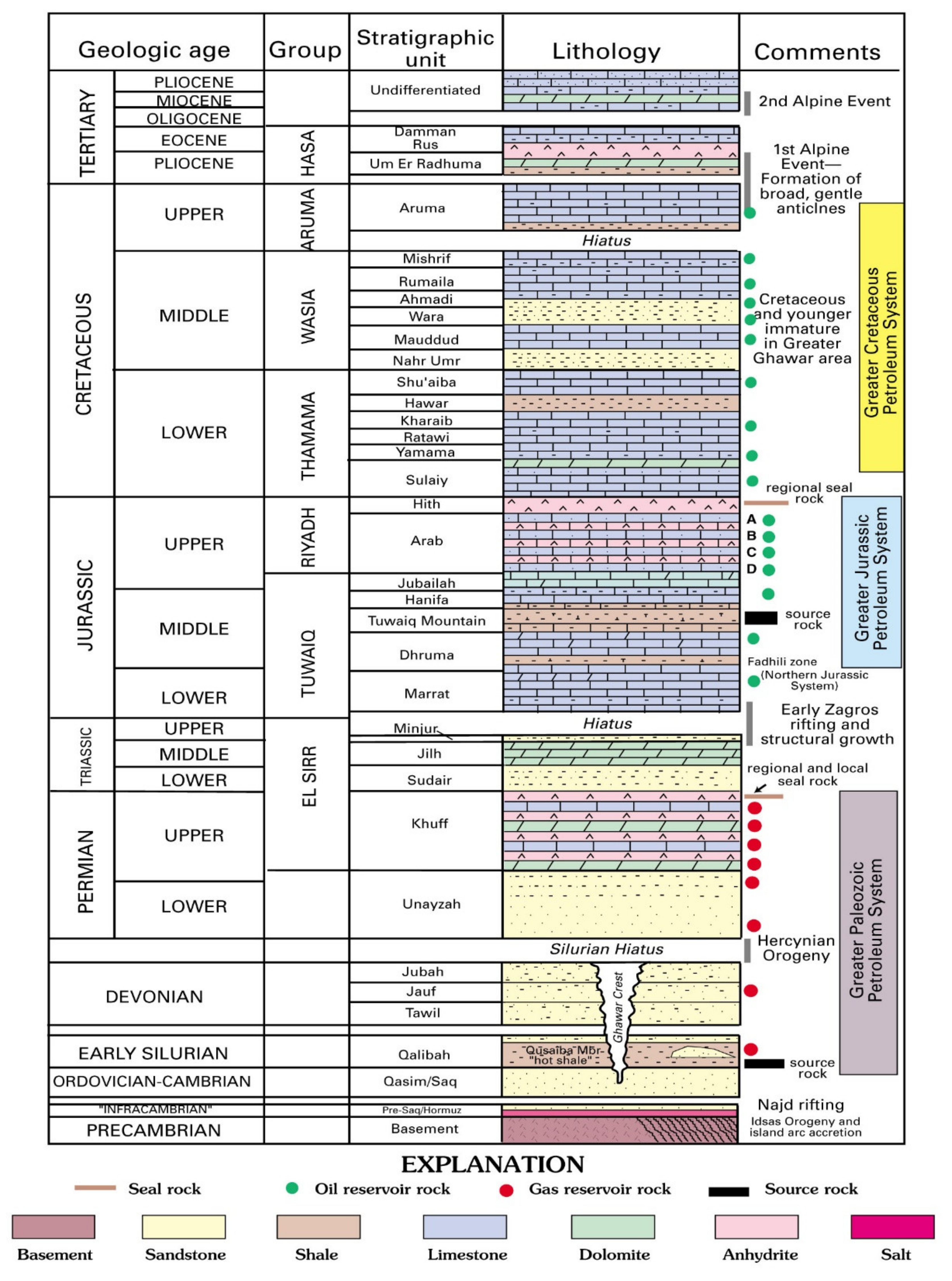
2. Geology of the Rub’ Al-Khali Basin

Due to lack of outcrop exposure (except in the west margin), the Rub’ Al-Khali basin evolution is known only from geophysical data. Stewart [20] reported the process of development of structures in the Rub’ Al-Khali basin from the Late Precambrian to Neogene observed on seismic, magnetic, gravity, and well data. This data shows a relatively complete Phanerozoic succession with north–south and northwest–southeast trending basement structure (Figure 1B) that are formed during East African Antarctic Orogeny. The structural trend in the Rub’ Al-Khali basin has been affected and reactivated during several periods including Ediacaran—Cambrian Ara/Hormuz salt, Devonian to Late Carboniferous Hercynian orogeny, early Mesozoic Gondwana break up, and finally in the Late Cretaceous and Tertiary time due to effects of the Arabian plate colliding with the Eurasian plate, resulting in the emplacement of ophiolites in the Oman Mountains.

3. Development of Digital Depth Models

There are almost no published data about the eastern parts of the Rub’ Al-Khali basin in Saudi Arabia. Only limited published data on the geological or geophysical properties were available for the Rub’ Al-Khali basin in Saudi Arabia. In this study, we performed an extensive literature review to compile one geophysical and geological model in the eastern Rub’ Al-Khali area using references specific to Rub’ Al-Khali. In cases where data are not available in these references, we obtain the missing data from references studying the same formations in nearby areas of Saudi Arabia, UAE, or Oman. In terms of geologic column in the Rub’ Al-Khali basin, we found the following twenty-three formations: Quaternary (F-1), Hofuf Dam Hadrukh (F-2), Dammam (F-3), Rus (F-4), Umm Er Radhuma (F-5), Aruma (F-6), Wasia (F-7), Shuaiba (F-8), Biyadh (F-9), Hith (F-10), Arab (F-11), Hanifa & Tuwaiq Mountain (F-12), Dhruma (F-13), Marrat (F-14), Minjur (F-15), Jilh (F-16), Sudair (F-17), Khuff (F-18), Unayzah (F-19), Qusaiba (F-20), Qasim (F-21), Saq (F-22), and Basement (F-23) (Figure 2). Eventually, twenty-three layers and two major faults were defined and digitized at variable intervals (Figure 2). The Phanerozoic stratigraphy column of the eastern Arabian Peninsula is given in Figure 3 [25]. The stratigraphy of layers and faults of the model were built mostly based on the geologic information provided by [19]. The elastic properties such as densities and velocities were determined using median values from digitized well-log data provided by several published articles as reported in Table 1 [18,22,23,26,27,28,29,30,31,32,33,34], and available Vp and density data were plotted in Figure 4. If logs are not available, values for these parameters from nearby areas are used. Due to the lack of availability of S-wave velocities for some formations, we use Vp-Vs relations to complete the whole stratigraphic column. We used the relation developed by [26] for carbonate lithologies, and relations presented by [22] for sandstones and shales. The remaining properties, which are P- and S-wave quality factors (Qp and Qs), were calculated using a method proposed by [27], which involves taking the square root of the corresponding value of P- and S-wave, respectively. The complete geophysical properties including P-wave velocity, S-wave velocity, density, lithology, P- and S- wave quality factors of each formation are listed in Table 1. Moreover, Figure 5 shows plots of the compiled Vp, Vs, ρ, Qp, and Qs models.

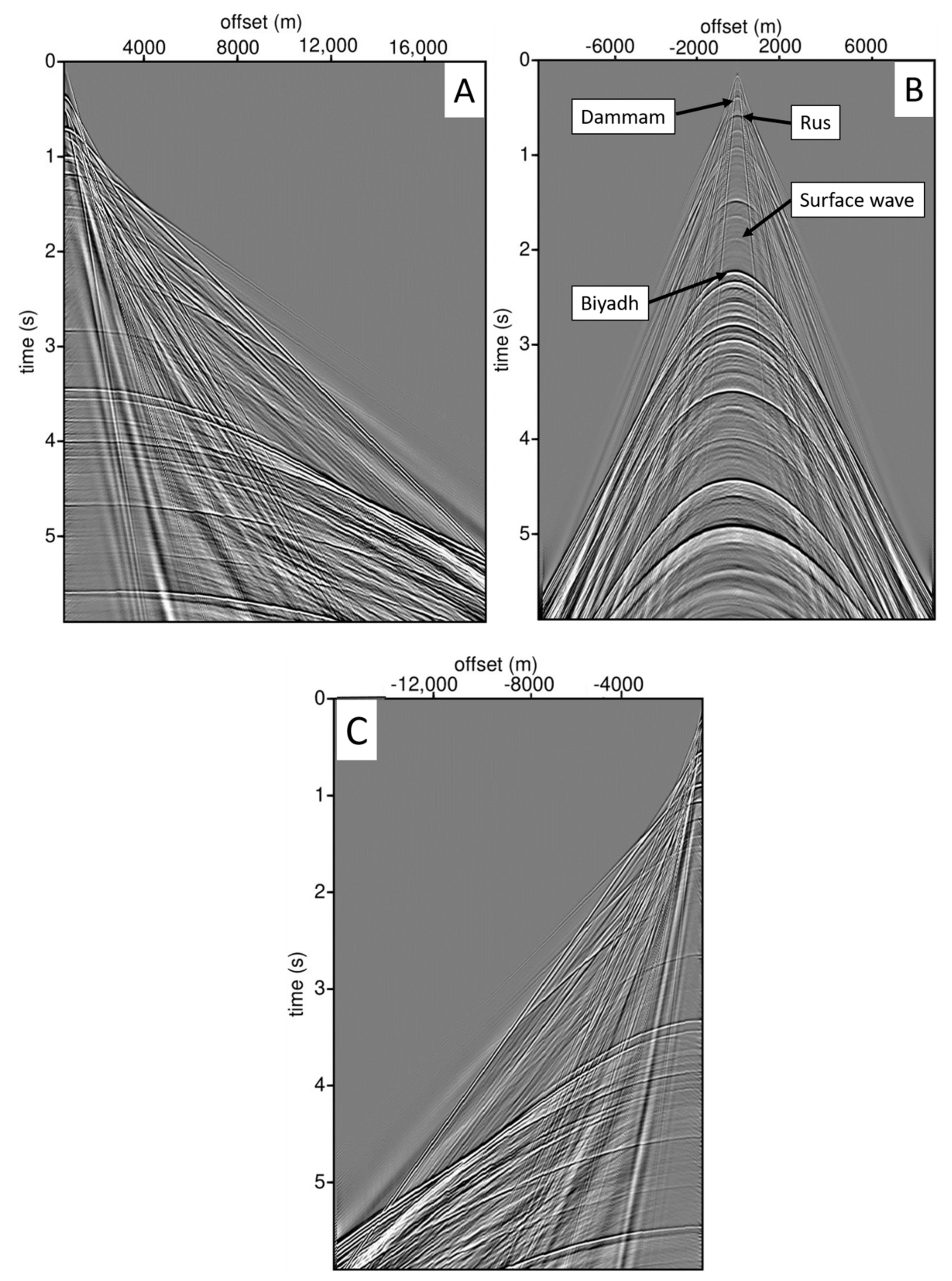
4. The Synthetic Seismic Data Generation Procedure

We apply 2D finite-difference approximation methodology to calculate the synthetic seismic data, using the available viscoelastic model inputs. This method involves the application of 2D wave equation to simulate the propagation of seismic waves in viscoelastic media that is determined by a modified Newton’s equation of motion and Hooke’s law, as described in [35,36]. We propagate the waves in a 2D viscoelastic medium by computing the 3 strain tensor components along the x-axis and z-axis, and also compute their associated stress tensors. Then, we calculate the divergence of the stresses which generate accelerations that are further extrapolated to produce displacements to succeeding time steps. The finite-difference method used here utilizes staggered grids to compute the spatial derivatives using the centered finite-difference approximations. The finite-difference algorithm inputs the viscoelastic properties (i.e., Vp, Vs, Qp, and Qs) from the compiled models to compute Lame’s coefficients and the wave’s relaxation parameters.
The finite-difference viscoelastic scheme begins with generation and propagation of the source at an initial time t = 0. Then it computes the wave-speeds using the finite-difference scheme by increasing time in little time steps while modifying the wave-speed in both x and z-directions, respectively. Subsequently, this process updates the stress field and makes it staggered in time relative to particle wave-speed fields. The process is repeated with another time step, updating the particle wave-speeds in this case until it covers the entire grid. At the boundaries of the grid, we utilize absorbing boundary conditions to minimize the effects of reflections. Usually, the computation of the finite-difference solutions relies on the frequency band of the source wavelet. In this case, we apply a typical Ricker wavelet having a zero-phase and a 20-Hz peak frequency. The finite-difference solution of the wave equation is usually associated with numerical dispersion if appropriate grid spacing is not used. To avoid this problem, we apply the general formula for preventing dispersion in the finite-difference scheme with accuracy close to spatial fourth-order and close to second order in time. This means that we must have a minimum of five grid points for every wavelength within a viscoelastic finite-difference scheme [37]:
Δ x   =   Δ z     V min 5 f max = 1.5   m
The grid sizes Δ x (along x-axis) and Δ z (along z-axis) are assumed to be equal, Vmin is the minimum wave speed, and fmax is the maximum frequency. In our model, Vmin = 501 m/s corresponding to the minimum shear-wave speed and fmax = 60 Hz, which is the frequency at which the wavelet amplitude spectrum drops below 1% of its maximum value. Consequently, we calculate a value of x = z = 1.5625 m, which is approximated to 1.5 m. Besides the dispersion criteria, the time-marching step of the finite-difference also needs to fulfill the Courant-Friedrichs-Lewy (CFL) stability criteria for convergence in 2D media [37], which is given as:
Δ t     Δ z   0.606 Δ x V max = 0.14   msec
where Vmax is the maximum wave speed in the model. We use the basement compressional-wave speed as the maximum velocity (i.e., Vmax = 6380 m/s), then we compute the time step as t = 0.142853 ms, which is approximated to 0.14 ms. All these parameters are embedded in the 2D finite-difference wave field modelling open-source code [37], which we utilized for generating the viscoelastic synthetic seismic data. To satisfy the boundary conditions, we used absorbing criteria with a taper of 375 grid points at the bottom, right, and left edges of the model and a free-surface boundary condition for the top margin of the model. We compute the taper using the formula described in [37]:
Taper   =   4 V max Δ x × f max = 375
Regarding the data acquisition, we apply a conventional 2D seismic land survey geometry. Starting from point x = 0 m, sources cover the whole horizontal length to point x = 40,000 m with a source interval of 50 m. Similarly, receivers cover a horizontal length from point x = 0 m to point x = 40,000 m, but with a receiver separation of 25 m. Receivers and shots are placed at 15 m depth below the top interface [37] to avoid the free-surface effect. The offset ranges from −40,000 to 40,000 m, which is desirable for most seismic data analysis and processing such as; velocity analysis, anisotropy, and amplitude variation with offset (AVO) analysis. Parameters used for the generation of synthetic seismic data sets are tabulated and presented in Table 2. We generated both horizontal and vertical components of the synthetic viscoelastic seismic data sets. Samples of the vertical component and horizontal component of displacements recorded at the beginning, center, and end of the model are presented in Figure 6 and Figure 7, respectively.
For generating the synthetic seismic data, we used a PC workstation running a Linux operating system with an Intel® Xeon® Processor E5-2687 3.0 GHz 10C and a memory of 256 GB 2133 MHz DDR4 ECC RDIMM. A single shot gather consumed approximately 36 h to generate on this workstation. We attribute this length to the relatively low minimum velocity and high maximum frequency of our model.

5. Conclusions

We have put together a 2D viscoelastic model from the eastern Rub’ Al-Khali basin and produced the associated dual-component synthetic seismic data sets. Regardless of the large number of layers involved in the model, the data appears to have good quality in capturing most important reservoirs including the relatively deep Khuff Formation. We provided the geologic model and associated seismic data sets, available online publicly for those who want to test their methods, and we encourage them to make their output open publicly too.

Author Contributions

Conceptualization, S.A.C., P.E., S.K., A.L.A. and A.A.A.-S.; methodology, S.A.C., P.E., S.K., A.L.A. and A.A.A.-S.; software, S.A.C., P.E., S.K., A.L.A. and A.A.A.-S.; validation, S.A.C., P.E., S.K., A.L.A. and A.A.A.-S.; formal analysis, S.A.C., P.E., S.K., A.L.A. and A.A.A.-S.; investigation, S.A.C., P.E., S.K., A.L.A. and A.A.A.-S.; resources, S.A.C., P.E., S.K., A.L.A. and A.A.A.-S.; data curation, S.A.C., P.E., S.K., A.L.A. and A.A.A.-S.; writing—original draft preparation, S.A.C., P.E., S.K., A.L.A. and A.A.A.-S.; writing—review and editing, S.A.C., P.E., S.K., A.L.A. and A.A.A.-S.; visualization, S.A.C., P.E., S.K., A.L.A. and A.A.A.-S. All authors have read and agreed to the published version of the manuscript.

Funding

This research received funding from the College of Petroleum Engineering and Geosciences of KFUPM through Startup Fund Grant number SF 18060.

Institutional Review Board Statement

Not applicable.

Informed Consent Statement

Not applicable.

Data Availability Statement

Publicly available datasets were analyzed in this study. This data can be found here: [https://www.dropbox.com/sh/9t099hhn1h8nea8/AAChpqVg3R_km2MlEMJ0SuxLa?dl=0].

Acknowledgments

The authors appreciate and acknowledge the support provided by King Fahd University of Petroleum and Minerals (KFUPM) by providing all the essential resources to conduct this study.

Conflicts of Interest

The authors declare no conflict of interest.

References

  1. Li, Q.; Wu, G.; Wu, J.; Duan, P. Finite difference seismic forward modeling method for fluid–solid coupled media with irregular seabed interface. J. Geophys. Eng. 2019, 16, 198–214. [Google Scholar] [CrossRef] [Green Version]
  2. Wang, J.; Hong, L. Stable optimization of finite-difference operators for seismic wave modeling. Studia Geophys. Geod. 2020, 64, 452–464. [Google Scholar] [CrossRef]
  3. Liu, J.; Yong, W.A.; Liu, J.; Guo, Z. Stable Finite-Difference Methods for Elastic Wave Modeling with Characteristic Boundary Conditions. Mathematics 2020, 8, 1039. [Google Scholar] [CrossRef]
  4. Wang, Y.; Ning, Y.; Wang, Y. Fractional Time Derivative Seismic Wave Equation Modeling for Natural Gas Hydrate. Energies 2020, 13, 5901. [Google Scholar] [CrossRef]
  5. Maranzoni, A.; Mignosa, P. Seismic-generated unsteady motions in shallow basins and channels. Part II: Numerical modelling. Appl. Math. Model. 2019, 68, 712–731. [Google Scholar] [CrossRef]
  6. Xu, Y.; Chen, X.; Han, D.; Zhang, W. Complex topography and media implementation using hp-adaptive DG-FEM for seismic wave modeling. EGU General Assembly 2020, Lund, Sweden, Online, 4–8 May 2020, EGU2020-21047. Available online: https://meetingorganizer.copernicus.org/EGU2020/EGU2020-21047.html (accessed on 1 June 2020).
  7. Asfour, K.; Martin, R.; El Baz, D. Numerical Modeling of Attenuation and Nonlinear Effects in Computational Seismology. EGU General Assembly Conference Abstracts. 2020, p. 91. Available online: https://ui.adsabs.harvard.edu/abs/2020EGUGA..22...91A/abstract (accessed on 1 June 2020).
  8. Jiang, C.; Zhou, H.; Xia, M.; Chen, H.; Zhang, Y.; Jiang, S. Acoustic Wave Simulation by Lattice Boltzmann Method with D2Q5 and D2Q9 of Different Relaxation Times. In Proceedings of the 81st EAGE Conference and Exhibition, London, UK, 3–6 June 2019; European Association of Geoscientists & Engineers: Houten, The Netherlands, 2019; pp. 1–5. [Google Scholar] [CrossRef]
  9. Sakemi, Y.; Hitoshi Mikada, J.T. A quantitative analysis of the passive seismic emission tomography using the lattice Boltzmann method. In Proceedings of the Japan Geoscience Union Meeting, Chiba, Japan, 26–30 May 2019; p. STT42–P04. [Google Scholar]
  10. Mora, P.; Morra, G.; Yuen, D.A. A concise python implementation of the lattice Boltzmann method on HPC for geo-fluid flow. Geophys. J. Int. 2020, 220, 682–702. [Google Scholar]
  11. Khan, S.; Khulief, Y.A.; Al-Shuhail, A. Mitigating climate change via CO2 sequestration into Biyadh reservoir: Geomechanical modeling and caprock integrity. Mitig. Adapt. Strateg. Glob. Chang. 2019, 24, 23–52. [Google Scholar] [CrossRef]
  12. Khan, S.; Al-Shuhail, A.; Khulief, Y.A. Numerical modeling of the geomechanical behavior of Ghawar Arab-D carbonate petroleum reservoir undergoing CO2 injection. Environ. Earth Sci. 2016, 75, 1499. [Google Scholar] [CrossRef]
  13. Khan, S.; Khulief, Y.A.; Al-Shuhail, A. The effect of injection well arrangement on CO2 injection into carbonate petroleum reservoir. Int. J. Glob. Warm. 2018, 14, 462–487. [Google Scholar] [CrossRef]
  14. Khan, S.; Khulief, Y.A.; Al-Shuhail, A. Numerical modeling of the geomechanical behavior of Biyadh reservoir undergoing CO2 injection. Int. J. Geomech. 2017, 17, 04017039. [Google Scholar] [CrossRef]
  15. Carcione, J.; Poletto, F.; Farina, B.; Craglietto, A. Simulation of seismic waves at the earth’s crust (brittle-ductile transition) based on the Burgers model. Solid Earth 2014, 5, 1001. [Google Scholar] [CrossRef] [Green Version]
  16. Soliman, F.; Al Shamlan, A. Review on the geology of the Cretaceous sediments of the Rub’al-Khali, Saudi Arabia. Cretac. Res. 1982, 3, 187–194. [Google Scholar] [CrossRef]
  17. Nairn, A.; Alsharhan, A. Sedimentary Basins and Petroleum Geology of the Middle East; Elsevier: Amsterdam, The Netherlands, 1997. [Google Scholar]
  18. Alfara, M.N.; Nebrija, E.L.; Ferguson, M.D. The Challenge of Interpreting 3-D Seismic in Shaybah Field, Saudi Arabia. GeoArabia 1998, 3, 209–226. [Google Scholar]
  19. Stewart, S.; Reid, C.; Hooker, N.; Kharouf, O. Mesozoic siliciclastic reservoirs and petroleum system in the Rub’Al-Khali basin, Saudi Arabia. Aapg Bull. 2016, 100, 819–841. [Google Scholar]
  20. Stewart, S. Structural geology of the Rub’Al-Khali Basin, Saudi Arabia. Tectonics 2016, 35, 2417–2438. [Google Scholar] [CrossRef]
  21. Al-Shuhail, A.A.; Mousa, W.A.; Alkhalifah, T. KFUPM-KAUST Red Sea model: Digital viscoelastic depth model and synthetic seismic data set. Lead. Edge 2017, 36, 507–511. [Google Scholar] [CrossRef] [Green Version]
  22. Al-Shuhail, A.A.; Alshuhail, A.A.; Khulief, Y.A.; Salam, S.A.; Chan, S.A.; Ashadi, A.L.; Al-Lehyani, A.F.; Almubarak, A.M.; Khan, M.Z.U.; Khan, S.; et al. KFUPM Ghawar digital viscoelastic seismic model. Arab. J. Geosci. 2019, 12, 245. [Google Scholar] [CrossRef]
  23. Khan, A.M.; Al-Juhani, S.G.; Abdul, S. Digital Viscoelastic Seismic Models and Data Sets Of Central Saudi Arabia in the Presence of Near-Surface Karst Features. J. Seism. Explor. 2020, 29, 15–28. [Google Scholar]
  24. Zhou, H.W. Multi-scale tomography for crustal P and S velocities in southern California. Pure Appl. Geophys. 2004, 161, 283–302. [Google Scholar] [CrossRef]
  25. Pollastro, R.M. Total Petroleum Systems of the Paleozoic and Jurassic, Greater Ghawar Uplift and Adjoining Provinces of Central Saudi Arabia and Northern Arabian-Persian Gulf; US Geological Survey; US Department of the Interior: Washington, DC, USA, 2003; p. 2202-H.
  26. Ameen, M.S.; Smart, B.G.; Somerville, J.M.; Hammilton, S.; Naji, N.A. Predicting rock mechanical properties of carbonates from wireline logs (A case study: Arab-D reservoir, Ghawar field, Saudi Arabia). Mar. Pet. Geol. 2009, 26, 430–444. [Google Scholar] [CrossRef]
  27. Mittet, R. A simple design procedure for depth extrapolation operators that compensate for absorption and dispersion. Geophysics 2007, 72, S105–S112. [Google Scholar] [CrossRef]
  28. Bridle, R.; Ley, R.; Al-Mustafa, A. Near-surface models in Saudi Arabia. Geophys. Prospect. 2007, 55, 779–792. [Google Scholar] [CrossRef]
  29. Liu, L.; Kharji, M.; Chatterjee, H.S. Seismic attributes as exploration tools: A case study from the Jurassic in Saudi Arabia. In Proceedings of the IPTC 2013: International Petroleum Technology Conference, Beijing, China, 26–28 March 2013; European Association of Geoscientists & Engineers: Houten, The Netherlands, 2013; p. cp–350. [Google Scholar]
  30. Dasgupta, S.N.; Hong, M.R.; La Croix, P.; Al-Mana, L.; Robinson, G. Prediction of reservoir properties by integration of seismic stochastic inversion and coherency attributes in super Giant Ghawar field. In SEG Technical Program Expanded Abstracts 2000; Society of Exploration Geophysicists: Tulsa, OK, USA, 2000; pp. 1501–1505. [Google Scholar]
  31. Macrides, C.G.; Kelamis, P.G. A 9C-2D land seismic experiment for lithology estimation of a Permian clastic reservoir. GeoArabia 2000, 5, 427–440. [Google Scholar]
  32. Al-Ahmadi, M.E. Hydrogeology of the Saq aquifer northwest of Tabuk, northern Saudi Arabia. Earth Sci. 2009, 20, 15. [Google Scholar] [CrossRef]
  33. Mooney, W.D.; Gettings, M.E.; Blank, H.R.; Healy, J.H. Saudi Arabian seismic-refraction profile: A traveltime interpretation of crustal and upper mantle structure. Tectonophysics 1985, 111, 173–246. [Google Scholar] [CrossRef]
  34. Sharland, P.; Archer, R.; Davies, R.B.; Simmons, M.D.; Sutcliffe, O.E. Arabian Plate Sequence Stratigraphy; GeoArabia Special Publication: Tysons, VA, USA, 2001; Volume 2, p. 371. [Google Scholar]
  35. Robertsson, J.O.; Blanch, J.O.; Symes, W.W. Viscoelastic finite-difference modeling. Geophysics 1994, 59, 1444–1456. [Google Scholar] [CrossRef] [Green Version]
  36. Talukdar, K.; Behera, L. Sub-basalt Imaging of Hydrocarbon-Bearing Mesozoic Sediments Using Ray-Trace Inversion of First-Arrival Seismic Data and Elastic Finite-Difference Full-Wave Modeling Along Sinor–Valod Profile of Deccan Syneclise, India. Pure Appl. Geophys. 2018, 175, 2931–2954. [Google Scholar] [CrossRef] [Green Version]
  37. Thorbecke, J. Finite-Difference Wavefield Modeling; 2016. [Google Scholar]
Figure 1. (A) Satellite image showing the location of the Rub’ Al-Khali basin. (B) Top basement depth structure map [20].
Applsci 11 01401 g001
Figure 2. Digitized 2D model of the Rub’ Al-Khali basin. Solid curves indicate horizons while dotted lines indicate faults.
Applsci 11 01401 g002
Figure 3. Phanerozoic stratigraphy column of the eastern Arabian Peninsula [25].
Applsci 11 01401 g003
Figure 4. Vp and ρ plot of selected formations [18,30,31,34].
Applsci 11 01401 g004
Figure 5. (a) Vp model; (b) Vs model; (c) density model; (d) Qp model; (e) Qs model.
Applsci 11 01401 g005aApplsci 11 01401 g005b
Figure 6. Vertical component of synthetic seismic data for shot located at (A) x = 1 m, (B) x = 2000 m, and (C) x = 40,000 m. Some prominent seismic events are indicated on (B).
Applsci 11 01401 g006
Figure 7. Horizontal component of synthetic seismic data for shot located at (A) x = 1 m, (B) x = 2000 m, and (C) x = 40,000 m.
Applsci 11 01401 g007
Table 1. Lithology, densities, compressional and shear-wave speeds, compressional and shear wave quality factors of layers of the eastern Rub’ Al-Khali basin model.
LayerFormationLithologyρ
(kg/m3)
Vp
(m/s)
Vs
(m/s)
QpQs
F-1QuaternarySand1500 a850 a501 a29.15 i22.36 i
F-2Hofuf Dam HadrukhMixed limestone and siliciclastic1877 b1835 b1180 c42.84 i34.35 i
F-3DammamLimestone2289 b3110 b1870 d55.77 i43.24 i
F-4RusAnhydrite2397 b5252 b2470 d65.32 i49.70 i
F-5Umm Er RadhumaLimestone2028 b3318 b1978 d57.60 i44.47 i
F-6ArumaLimestone2037 b3558 b1672 d52.25 i40.89 i
F-7WasiaSandstone2277 b3233 b2142 c56.86 i46.28 i
F-8ShuaibaLimestone2037 b3010 b1818 d54.86 i42.63 i
F-9BiyadhSandstone2364 b4045 b2701 c63.60 i51.97 i
F-10HithAnhydrite2874 e4483 e2328 e66.96 i48.24 i
F-11ArabLimestone2400 e5399 e2748 e73.47 i52.42 i
F-12Hanifa & Tuwaiq MountainLimestone25505698 e,k2903 e75.48 i53.88 i
F-13DhrumaLimestone2458 f,k5033 f,k2870 d70.94 i53.57 i
F-14MarratShale2410 f3272 f1436 c57.20 i37.89 i
F-15MinjurSandstone2394 f3930 f2499 c62.69 i49.99 i
F-16JilhDolomite2400 f,k4823 f,k2761 d69.45 i52.54 i
F-17SudairShale2372 g,k5182 g,k2674 g71.99 i51.71 i
F-18KhuffDolomite2639 g,k4953 g,k2530 g70.38 i50.3 i
F-19UnayzahSandstone2405 g3752 g2085 g61.25 i45.66 i
F-20QusaibaShale2486 g3898 g2143 g62.43 i46.29 i
F-21QasimSandstone2380 h3685 h2453 c60.70 i49.53 i
F-22SaqSandstone2350 h3765 h2508 c61.36 i50.08 i
F-23BasementIgneous and metamorphic2800 j6380 j3580 j79.87 i59.83 i
a [28], b [18], c [22,23], d [26], e [29], f [30], g [31], h [32], i [27], j [33], k [34].
Table 2. List of parameters used to construct synthetic seismic data.
ParameterValue
Source wavelet20 Hz zero-phase Ricker
Time sampling interval for finite-difference calculation0.14 ms
Square-grid size for finite-difference calculation1.5 m
Receiver spacing25 m
Shot spacing50 m
Recording time sampling interval4.0 ms
Total recording time6.0 s
Total number of receivers1535
Receivers x-axis0 to 40,000 m
Receivers z-axis15 m
Shots x-axis0 to 40,000 m
Shots z-axis15 m
Offset range−40,000 to 40,000 m
Total number of shots801 shots
Publisher’s Note: MDPI stays neutral with regard to jurisdictional claims in published maps and institutional affiliations.

