Abstract
Due to the approved applicability of differential evolution (DE) in geophysical problems, the algorithm has been widely concerned. The DE algorithms are mostly applied to solve the geophysical parametric estimation based on specific models, but they are rarely used in solving the physical property inverse problem of geophysical data. In this paper, an improved adaptive differential evolution is proposed to solve the norm magnetic inversion of 2D data, in which the perturbation direction in the mutation strategy is smoothed by using the moving average technique. Besides, a new way of updating the regularization coefficient is introduced to balance the effect of the model constraint adaptively. The inversion results of synthetic models demonstrate that the presented method can obtain a smoother solution and delineate the distributions of abnormal bodies better. In the field example of Zaohuoxi iron ore deposits in China, the reconstructed magnetic source distribution is in good agreement with the one inferred from drilling information. The result shows that the proposed method offers a valuable tool for magnetic anomaly inversion.
1. Introduction
The magnetic method is widely used in mineral resource exploration and structure investigation. To determine the depth, position, and shape of the magnetic anomaly body, the magnetic data inversion is usually needed, which mainly includes parameter inversion [1,2], imaging inversion [3,4,5], and physical property inversion [6]. Physical property inversion can recover the shape and depth of complex sources without depending on a specific model. Therefore, the inversion of physical properties has become one of the most important and commonly used methods. Linear iterative methods, such as the steepest descent method, Newton’s method, and conjugate gradient method, are usually used in physical property inversion [7,8,9]. However, the gradient-based algorithms are independent of the initial guess to start the optimization process and are easy to trap into local minima for nonlinear problems [10]. Contrary to the conventional approaches, the metaheuristic methods like differential evolution (DE) do not require good initial solutions when searching the global minimum.
DE [11] is a population-based metaheuristic global optimization algorithm. Because of its fast convergence and easy implementation, it has been widely used to solve the optimization of practical problems, such as electromagnetic optimization [12,13], pattern recognition [14], signal processing [15,16,17,18,19,20], engineering application [21,22,23], and other inversion problems [24,25,26,27]. Considering the dependency of control parameters [28], some scholars tried to adjust them by using adaptive or self-adaptive manners.
Liu and Lampinen proposed an adaptive DE based on fuzzy logic (FADE) [29]. Brest optimized the scaling factor (F) and crossover rate (CR) by encoding them into individuals as parameters [30]. Zhang and Sanderson automatically adjust F and CR based on historical experience information, then proposed an adaptive DE with an optional external archive (JADE) [31]. In JADE, F, and CR are generated based on Cauchy distribution and Gaussian distribution, respectively. Besides, JADE introduces a new mutation strategy named “current-to-pbest”, which can balance the global exploration and local exploitation capability of the algorithm better than the traditional ones. Then, researchers have proposed success-history based DE (SHADE) by improving the technique of the parameter adjustment in JADE [32]. In recent years, a series of DE algorithms with superior performance have been presented based on SHADE, such as using linear population size reduction to improve the search performance of SHADE (LSHADE) [33], improved LSHADE algorithm (iLSHADE) [34], ensemble sinusoidal differential covariance matrix adaptation with Euclidean neighborhood (LSHADE-EpSin) [35], LSHADE with semi-parameter adaptation hybrid with CMA-ES (LSHADESPACMA) [36], single objective real-parameter optimization algorithm (jSO) [37], etc.
DE has few applications in magnetic data inversion. For example, some scholars first applied DE into 3D inversion of the magnetic anomaly to estimate the source parameters such as the horizontal extension, the depth of top and bottom interface, the magnetic dip, and declination [38]. Other scholars have applied DE to analytic signal amplitude (ASA) inversion of two-dimensional (2D) magnetic data [39]. As far as magnetic inversion is concerned, there is a huge difference between the observed data and the inverted parameters, which means that one needs to recover a large number of model parameters by using a small amount of physical field information. Hence, the magnetic inversion is ill-conditioned and exists in multiple solutions. To address the mentioned issues, it is necessary to add the prior information as a constraint to reduce non-uniqueness and make the calculated model as close to the real one as possible. In addition, since the forward modeling calculation in this paper is based on the finite volume method, the relation of magnetic source parameters and magnetic data is nonlinear. The norm based objective function aggravates the non-linearity further.
This article has systematically studied the () norm inversion of the magnetic data based on the proposed adaptive DE. The proposed algorithm can improve the global search ability and solution precision. Besides, considering that the original DE failed to obtain a smooth model, we designed a new mutation strategy to solve this problem. Although the inversion regularized with norm has been widely solved by applying the gradient-based methods [40,41,42,43,44], the application of adaptive DE in the physical property of magnetic data is studied for the first time.
2. Method
2.1. Conventional Differential Evolution Algorithm
(1) Initialization
Like other evolution algorithms (EAs), DE initializes the population within a given search range in a certain way, such as uniform random initialization, chaos initialization, opposition learning initialization, clustering initialization, etc. [45,46,47,48,49]. In the conventional DE algorithm, the population size (NP) with D dimension is initialized as follows:
where and are the upper and lower bounds of the -th variable, respectively, generates a random number between [0, 1] according to a uniform distribution, and G represents the generation number of the evolutionary search.
(2) Mutation
After the initialization, a mutant vector will be created for each target vector according to the mutation strategy. The most widely used mutation strategies are listed as follows [50,51],
“DE/rand/1”:
“DE/rand/2”:
“DE/best/1”:
“DE/best/2”:
“DE/current-to-best/1”:
“DE/current-to-pbest/1”:
where is the individual vector, which has the best fitness value at the current generation. were mutually different random integers between 1 and NP. F is a scale factor within the range of (0, 1].
(3) Crossover
In DE, to obtain the trial vector by replacing certain variables of the target vector with corresponding mutant vector , a crossover operation was needed. There were two types of crossover schemes: Exponential crossover and binominal crossover [33]. In the binominal crossover, the following formula is used to generate the trial vector,
where is the crossover rate that controls which or how many components were inherited from the mutant vector. was a randomly selected integer in the range [1, D] to ensure that one of the variables in the trial vector must come from the mutant vector.
(4) Selection
DE adopts a one-to-one selection method. The fitness value of the target and the trial vectors determine which one will be selected into the population of the next generation. The selection scheme is given by:
where is the fitness value of the target and the trial vectors.
2.2. Adaptive Adjustment of Control Parameters
In the conventional DE algorithm, F and CR are fixed values. Different problems usually need to set different parameters to obtain optimal performance of the algorithm. To avoid manually adjusting these parameters, it was an ideal strategy to adopt an adaptive method to update F and CR based on successful experience continuously. Considering that the improved DE algorithm shared the same architecture with JADE [31], in this part, a detailed description of parameters adjustment will be instructed.
Firstly, is defined as,
where denotes the Cauchy distribution with location parameter and scale parameter 0.1. If , it was regenerated by the execution of Equation (11) until an effective value was obtained; if , it was truncated to 1.0. The initial value of was 0.5. In the subsequent evolution process, it was updated according to the scale factor fed back from the successful individuals. At the end of each iteration, these successful are stored in the set , and is updated as follows,
where the learning rate c is a positive constant in the range ; is the Lehmer mean and calculated as follows,
In addition, each individual in JADE has an independent crossover rate in the range . Unlike , the generation of is controlled by the normal distribution,
where returns a random value with a normal distribution . If or , it is truncated to 0 or 1. is updated as follows [31],
where is the arithmetic mean; is the set of successful CR values in the current generation.
2.3. Improved Adaptive Differential Evolution Algorithm
The evolution algorithm has its advantages in solving non-smooth and non-differentiable problems. However, the inversion of magnetic data requires that the restored model is smooth and continuous in space. Therefore, it was necessary to improve the DE algorithm suitable for the optimization of magnetic inversion.
2.3.1. Initialization
Generally, the global search algorithm does not depend on the population initialization. Unfortunately, if the random initialization was carried out according to Equation (1), it will bring difficulties in determining the regularization coefficient. Therefore, the population in this paper was initialized randomly in a small range according to Algorithm 1.
| Algorithm1 Population Initialization |
| 01: For to Do 02: For to 03: 04: End For 05: End For |
2.3.2. Construction of the Smooth Matrix
There were many ways to establish smooth matrix S, such as moving average, Gaussian smoothing, k-nearest smoothing, median smoothing, etc. [52,53,54,55]. In this paper, the moving average method was adopted. For the model parameters , the adjacent elements in space are shown in Figure 1. Set the weight of each adjacent point , then the smoothed is
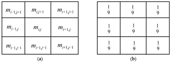
Figure 1.
The square-shaped window of . (a) The adjacent elements of , (b) the weight of adjacent position parameters of .
In order to reuse the above formula, the coefficients corresponding to all elements can be converted into sparse matrix . The -th row of matrix is used to store the weight information of neighborhood elements of -th cell. Finally, the smooth matrix is,
where is the time of smoothness, and the specific value should be determined by trial-and-error. In general, .
2.3.3. Mutation Strategy Based on the Smooth Search Direction
Due to the randomness of the nonlinear global search algorithm, the parameters obtained by inversion are usually discontinuous. Šešum and Tošić assumed that combining the smoothing filters with a genetic algorithm can improve the quality of obtained results [56]. However, Wu et al. believed that smoothing the individuals will reduce the population diversity [57]. Then, another smoothing strategy was proposed, which only smooths the model before the forward modeling calculation, and the smooth model did not replace the parameters in the original population. In addition, some scholars used the particle swarm optimization method to make the obtained solution closer to the designed model by smoothing the velocity direction of the particle [10]. In DE, we smoothed the individuals, which produced the differential direction. Let the smoothing matrix be , then the smooth vector of individual can be defined as,
Obviously, smooth difference vectors can be constructed by selecting different smooth vectors for all differential evolution mutation strategies. For simplicity, we only considered the “current-to-pbest/1” mutation strategy of Equation (12). When the smooth vector of an individual is used, it evolves into:
In the above formula, the difference vector formed by the pbest individual and the target vector does not use the smooth vector of the related individual because the convex combination property of and will be destroyed by the smooth process. At the same time, the mutant vector formed entirely based on the smooth vector will reduce the diversity of the population.
2.3.4. Improvement of the Selection Strategy
The disturbance direction of DE was generated by the smooth individual vector. When the target vector was replaced by its trial vector , the smooth vector also needs to be recalculated and stored, and Equation (14) is changed as,
From Equation (19), the selection operation of the improved DE algorithm should keep the trial vectors and store their corresponding smooth vectors.
2.3.5. Sorting Crossover Rate
The main function of sorting crossover rate was to prevent the rapid loss of excellent individuals. It also plays a role in preventing the average value of the crossover rate from rapidly decreasing. For more details, please refer to [58].
2.3.6. Other Related Adjustments
In this paper, , , the maximum number of estimates , was the number of the elements. Note that the and were inconsistent with those of the JADE algorithm. The existing study shows that the separable problems required a small crossover probability [59], while the inseparable problem required a larger crossover probability. Considering that the magnetic anomaly field was the comprehensive reflection of the subspace magnetic sources, it indicated that the objective function of magnetic data was inseparable. Therefore, it was more appropriate to maintain a larger crossover probability. In addition, maintaining a larger was helpful to improve the exploration of DE when using smooth vectors to generate the differential vector.
2.4. Magnetic Anomaly Inversion
2.4.1. Forward modeling of Magnetic Anomaly
In this paper, the finite volume method (FVM) was used to synthesize the magnetic anomaly data [60]. Let the forward modeling operator be , then the relationship between the observed data and the model parameter is defined as follows:
In the forward modeling process, the demagnetization effect was considered, although this effect was negligible for the sources of weak susceptibility.
2.4.2. The Construction of the Inverse Problem
The objective function of norm magnetic anomaly inversion can be expressed as follows,
λ is the regularization coefficient; is the data fitting objective function, which is generally norm; is the model objective function. In most inversion problems, is generally norm. Here, we consider the more general norm. are the range of the model parameters. If there are D optimized parameters, the upper and lower bounds of the model parameters are set as , . The data fitting objective function can be defined as,
where is the weighted matrix formed by the reciprocals of the noise in the observation data. In the above formula, the data fitting objective function used normalization processing to weaken the data errors’ influence on data fitting objective function [61]. Correspondingly, we define the model objective function as,
where is the weight coefficient of element , and used to store the prior information of the model, such as depth weighting [6]; is an initial model (the reference model or 0). Combining Equations (22) and (23), the objective function of magnetic inversion can be written as follows,
2.4.3. Adaptive Regularization Coefficient
The regularization coefficient λ controls the weight of the model objective function. Since the model objective function was all non-negative, its value range was . When λ = 0, the objective function only contains the data fitting term; when, the influence of the data fitting term can be ignored. Scholars proposed an adaptive regularization method based on the average fitness of the population [62]. Some scholars set the initial value of the regularization coefficient in a certain way at the beginning of the iteration [63] and then decreased the initial value continuously until λ less than a certain threshold. DE was a population-based search algorithm, which needs to combine the above two methods to constrain the inversion process effectively. Therefore, a new adaptive regularization coefficient scheme is proposed:
where is the average value of the data objective function of the Gth-generation in the population; ; when increases or does not change, it is necessary to reduce the regularization coefficient λ to weaken the influence of the model constraint term. The reason is that the EAs cannot ensure each model is updated. At the first iteration, the regularization coefficient is defined as,
where is the average value of the model constraint term.
2.4.4. Construction of the Model Weight Vector
(1) The depth weighting function
There are many depth weighting methods, and the method proposed in [6] is more commonly used. The depth weighting function can be expressed as,
where β is the attenuation index, for 2D magnetic inversion, β = 2 [10]; is a constant, which is related to the observation height of the measuring point; z is the depth of the element’s center. When p-norm is considered, the weighting coefficient of element i can be obtained by applying Equation (27):
(2) Weighting of element area
The area weighting matrix is a diagonal sparse matrix formed by the area of the element. For any element i, if the size of it is known to be , then,
When the element size of the inversion space is uniform, the area of each element is the same, which makes no sense to employ area weighting. However, when the inversion element was non-uniform, an area weighting matrix was necessary.
In summary, we have considered two kinds of model weight information, the weight coefficient of element i is,
where is the weight vector of the model. For example, the effect of depth weighting was to suppress the shallow elements and avoid model concentration near the surface.
2.4.5. Implementation of the Inversion Algorithm
In the above, we have discussed the objective function, adaptive regularization coefficient, mutation strategy based on a smooth vector of individual, and control parameters of adaptive DE. In this section, the adaptive DE algorithm for 2-D norm magnetic anomaly inversion was systematically presented. The flowchart of the DE algorithm is shown in Figure 2. Its main content includes the following parts:
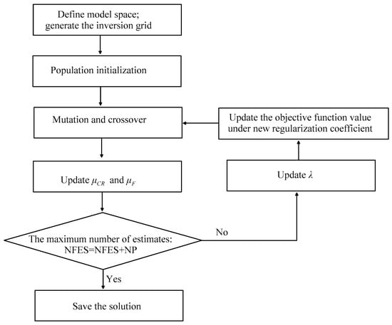
Figure 2.
Flowchart of the differential evolution (DE) algorithm for the inversion of magnetic data.
- (1)
- Load the observation data, and generate the inversion grid according to the inversion area. Store the coefficient sparse matrix related to the control equation for the forward modeling calculation. Create model weighted vectors and store them. The geomagnetic parameters related to magnetic anomaly are known.
- (2)
- Population initialization of DE: Given the population size and the initial and , and the population vector is initialized by Algorithm 1. Smooth the vectors of the population and store them, and initialize the Regularization coefficient by Equation (26).
- (3)
- Mutation and crossover: The variation vector is generated by Equation (18), and the trial vector is generated by Equation (8).
- (4)
- Selection and update of DE control parameters: The smooth trial vector is evaluated. According to Equation (19), to determine whether to update the population and the individual vector in the population . Update and according to Equations (14) and (11).
- (5)
- Termination condition: Judge whether the termination condition is satisfied. If it is true, the current inversion result will be output; otherwise, turn to step (6).
- (6)
- Update the regularization coefficient. If the regularization coefficient changes, it is necessary to update the objective function value of the population under the new regularization coefficient and turn to step (3).
The pseudo-code of the inversion Algorithm 2 is as follows:
| Algorithm 2 Norm Inversion Algorithm of Magnetic Anomaly Based on Improved DE |
| 01: Data preprocessing. Read in the observation data, and generate the inversion grid and forward modeling sparse matrix, and then generate the weight vector of the model 02: = 1; = 0 03: Set = 100, = 0.9, = 0.9,= 0.1. The population initialization based on Algorithm 1: Generate smooth populationInitialize the regularization coefficient 04: While termination conditions are not satisfied do 05: 06: For to do 07: 08: 09: End For 10: For do 11: Using the difference vector of smooth individuals, the mutation vector is generated according to the mutation strategy in Equation (18) 12: According to Equation (8), the trial vector is generated 13: End For 14: Evaluate the trial vector 15: According to Equation (19), the new populations and are formed. 16: Update and by Equations (14) and (11) 17: The maximum number of estimates 18. End While |
3. Model Inversion and Discussion
This section focuses on the influence of the mutation strategy, norm value, and the upper and lower bounds of magnetic parameters on the inversion results. For all theoretical models, without specified explanation, the magnetic inclination , line direction , geomagnetic field amplitude .
3.1. The Influence of Smoothness on Inversion Results
Two simple models were used to test the influence of smooth individual vectors on the inversion results. Figure 3a is the cross-section through the x-axis of a 2-D magnetic dyke model. The dyke was buried at a depth of 50 m and extended to 150 m. Figure 3b is the cross-section through the x-axis of a 2-D magnetic dyke model at a dip angle of 135°.
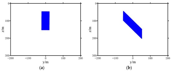
Figure 3.
The cross-section through the x-axis of the 2D models. (a) Model 1, (b) Model 2.
The norm p of the model objective function is 2, and only the positive constraint is imposed on the model, without the upper limit of magnetic susceptibility. The magnetic anomaly distribution of the model is shown in Figure 4.

Figure 4.
The tested models used for studying the effect of smooth vector strategy. (a) Model 1, (b) Model 2.
Figure 5 is the magnetic anomaly curve when the magnetic susceptibility was 0.01 . In order to ensure the accuracy of the simulation, the size of the forward model element was 5 × 5 m. During inversion, too many mesh sections will aggravate the ill-posedness of inversion. Therefore, the horizontal grid spacing was set as 10 m, and the grid spacing in the depth direction was a sparse grid that increased proportionally, and Algorithm 2 was used for inversion.
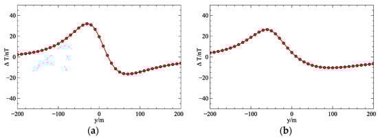
Figure 5.
Anormal magnetic field ∆T of Model 1 and 2. (a) Model 1, (b) Model 2.
In order to compare the conventional adaptive differential evolution and the improved one, the smooth and non-smooth inversion results are shown in Figure 6. It is not difficult to observe that the proposed algorithm was capable of obtaining better results than the original algorithm. Figure 6 shows that the continuity of the model was poor, the inversion results were divergent, and the background noise was strong without considering the smoothness. When , the recovery of the model was better than . It can also be found from the above two figures that the magnetic parameters recovered by the inversion were 0.01 lower than the theoretical values without adding upper bound constraint. The main reason for this phenomenon is that l2 norm inversion tends to obtain the smoothest model. For the abnormal body with a simple shape, the result can roughly reflect the dip information of the geologies. However, when the shape of the abnormal body tends to be complex, it can seldom depict the edge information of the model. In the following study, we set to smooth the individuals in the population by default.
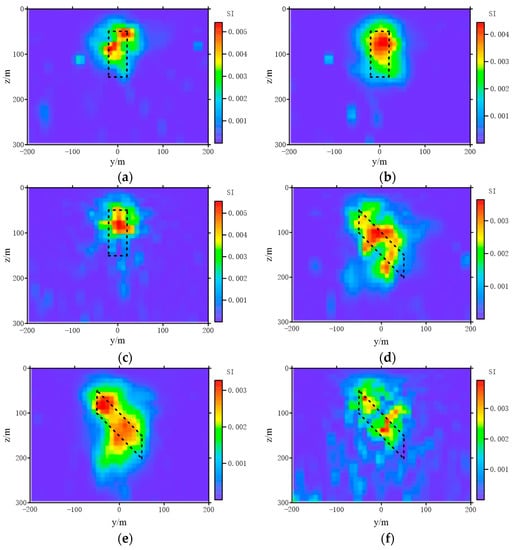
Figure 6.
The smooth and non-smooth inversion results of Model 1 and Model 2. (a) The smooth inversion of Model 1 (), (b) the smooth inversion of Model 1 (), (c) the non-smooth inversion of Model 1, (d) the smooth inversion of Model 2 (), (e) the smooth inversion of Model 2 (), (f) the non-smooth inversion of Model 2.
3.2. The Influence of P in Model Objective Function on Inversion Results
Figure 7 is the cross-section through the x-axis composed of two 2-D magnetic dyke models.
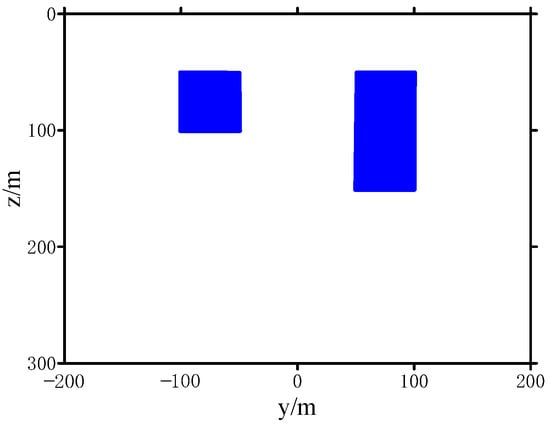
Figure 7.
The cross-section through the x-axis of the model.
Set the magnetic susceptibility χ = 0.01 SI and 0.02 SI. When p = 1.0, 1.1, 1.3, 1.5, 1.7, 2, we used Algorithm 2 to perform smooth inversion for Model 3 (Figure 8). The inversion results are shown in Figure 9. From the inversion results, we can observe that when p was large, the restored magnetic susceptibility was lower than the real value. The smaller p was, the closer the inversion result was to the real value. However, on the other hand, the larger p was, the larger the range of abnormal bodies distribution will be compared with the real model. Moreover, there will be interference between different anomalies to produce false anomalies. Generally speaking, was a suitable choice without the constraint of the upper bound of magnetic susceptibility. In Figure 10, due to the setting of the termination conditions, the field values obtained by inversion with each p-norm can fit the observed data. In summary, to balance the smoothness of the model and maintain the edge of the restored model, we set p = 1.2 in the subsequent work.
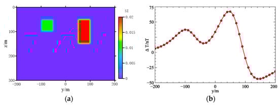
Figure 8.
Susceptibility model 3 and its ∆T field. (a) Spatial distribution of magnetic susceptibility of model 3, (b) the ∆T of model 3.
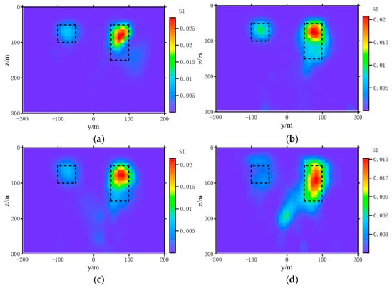
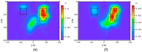
Figure 9.
The inversion results of model 3 by using different p value. (a) , (b) , (c) p = 1.3, (d) p = 1.5, (e) , (f) .
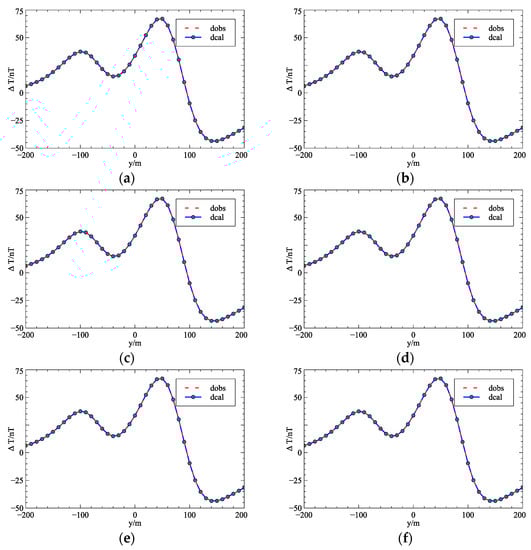
Figure 10.
The data reconstruction results of different p values. (a) , (b) , (c) , (d) , (e) , (f) .
3.3. Influence of Noise on the Inversion Results
In the objective function, noise suppression was realized by the data misfit term. In most cases, the norm value of the data objective function q equals 2. We add Gaussian white noise with the mean value of 0 and the standard deviation of the percentage of the abnormal amplitude. The forward modeling data of Model 3 are superimposed with different degrees of noise, and the data after adding noise is shown in Figure 11. The set maximum number of iterations is 100D. The inversion results are shown in Figure 12. With the increase of noise, the abnormal shape deviates from the real model, and false anomalies appear in the deep. In Figure 13, the observed data and predicted inversion results with different noises are compared. The inversion results can reflect the original shape of the observed data.
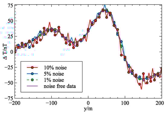
Figure 11.
The abnormal magnetic data of Model 3 with different noise level.
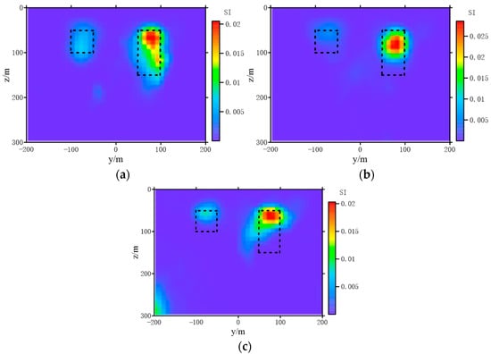
Figure 12.
The inversion results with different noise level. (a) 1% noise, (b) 5% noise, (c) 10% noise.
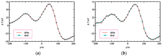
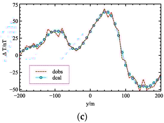
Figure 13.
The comparison of observed data and predicted results. (a) 1% noise, (b) 5% noise, (c) 10% noise.
4. The Inversion of Real Data
The synthetic data constructed in Section 3 refers to the actual geological data and previous results, which are in line with the actual situation. From the synthetic data tests, the inversion results of synthetic models show that this method can obtain smooth solutions and describe the distribution of anomalous bodies well. The previous sections have discussed the influence of p and smoothness on the inversion results. It is concluded that q = 2 and p = 1.2 are suitable for the norm smooth inversion of real data. However, the influence of the upper and lower bound constraints on the inversion results lacks discussion. Because some scholars have discussed in detail the influence of the parameters range on the results [43]. The inversion based on DE also has similar effects. The smaller the upper bound of the magnetic parameters, the larger the boundary of the recovered model, and on the contrary, the more concentrated they are. When dealing with real data, the upper and lower bound constraints need to be concerned.
The Zaohuoxi study area is located at the junction of the Qimantag suture zone and the North Kunlun magma arc zone. Most of the area is covered by Quaternary sediments with an average thickness of more than 60 m. The mineral resources in the area were mainly contact skarn-type iron polymetallic deposits. According to the work in [64], the highest magnetic susceptibility of the mineral in this region was magnetite with an average of 0.37 SI. At the same time, there was strong remanence with a maximum of 33.4 A/m in the study area. The magnetic parameters of minerals and rocks in the study area are shown in Table 1. The geomagnetic inclination and the geomagnetic field amplitude were 53.73° and 53,739 nT, respectively.

Table 1.
Magnetic parameters of minerals and rocks in the Zaohuoxi research area [64].
The drilling results show that there was magnetite with a small distribution range in line L, which is shown in Figure 14. The magnetic anomaly of line L is shown in Figure 15. The magnetic anomaly in the central and southern part of the study area was regular in shape and distributed in a north-west-west (NWW) band. The anomaly was positive in the south and negative in the north.
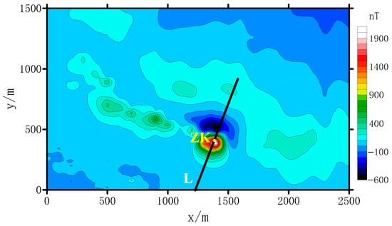
Figure 14.
The magnetic contour map of ∆T in the Zaohuoxi area. (ZK is the borehole position and L is the survey line).
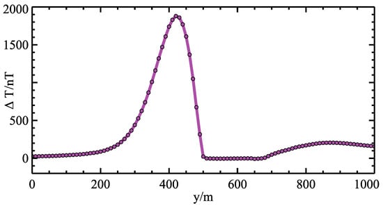
Figure 15.
The magnetic anomaly of line L.
The magnetic anomaly of line L has a sharp shape (in Figure 15), high intensity (the peak value up to 1980 nT), and a steep gradient. It is the strongest magnetic anomaly zone in the region. Ou et al. [64] constructed the underground distribution of the area based on the drilling and geology information, as shown in Figure 16.
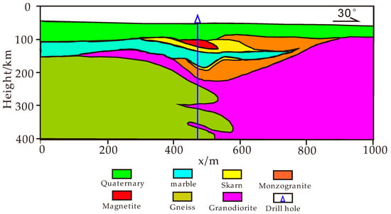
Figure 16.
The underground distribution of line L [64].
In Figure 16, the magnetite with a small distribution range, buried to a depth about 100 m, x = 450 m. The high magnetic anomaly corresponding to line L in this area was mainly caused by magnetite with magnetic susceptibility . In the following inversion, the upper bounds of susceptibility were set as 0.37, 0.74, and 1.21 , respectively. The inversion results are shown in Figure 17. From Figure 17, the inverse position of the magnetite was buried at about 100 m, and the horizontal position was also consistent with the information in the drill hole. It was shown that the inversion result of this method was reliable. The inversion results with the upper bound of magnetic susceptibility can highlight the distribution of abnormal bodies better. When the upper bound of magnetic susceptibility was large, the distribution of the abnormal bodies was reduced. At the same time, the larger the upper limit of magnetic susceptibility, the dip direction of the magnetic body will be affected by oblique magnetization and deviate to the magnetization direction.
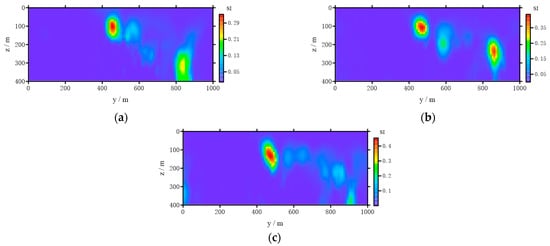
Figure 17.
The susceptibility image of ∆T for line L with different susceptibility constraints in the Zaohuoxi area. (a) , (b) , (c) .
To sum up, the constrained smooth inversion of magnetic anomaly data in the study area was carried out. The results show that the constrained inversion can better reveal the distribution of the magnetic bodies. However, this kind of constraint was still rough. A more reasonable constraint was needed by using the magnetic susceptibility of different depths and different lithologies or according to the known and reliable reference model.
5. Conclusions
In this paper, an improved DE algorithm is proposed to solve the norm inversion of 2D magnetic data. An adaptive regularization coefficient updating strategy for DE is proposed, and the mutation strategy of DE is improved by smoothing individual vectors. The proposed algorithm can obtain a smoother solution. The influence of smoothness and p in the model constraint term is analyzed. When there is more reliable constraint information, the smaller p can be used to highlight the model contour. As validated by synthetic models, this method can obtain a smoother solution and delineates abnormal bodies’ distribution. Finally, the method is used in real data in the Zaohuoxi area, China, and the inversion result is consistent with the drilling results.
However, the search efficiency of the DE algorithm is not compared with other algorithms, and it is difficult to compare the DE algorithm with other techniques like gradient-based algorithms and particle swarm optimization algorithms by applying a fair criterion. This work will be completed in future research. At the same time, the 2D of magnetic inversion is based on the assumption that the strike of the anomaly body is perpendicular to the inversion profile with infinite extension. In practical problems, this assumption will restrict the application of 2D inversion. Therefore, it is necessary to extend the inversion method based on the DE algorithm to a three-dimensional case.
Author Contributions
Conceptualization, W.D. and L.C.; methodology, L.C.; software, L.C.; validation, W.D.; formal analysis, W.D.; investigation, L.C.; resources, W.D.; data curation, L.C.; writing—original draft preparation, W.D.; writing—review and editing, L.C. and Y.L.; visualization, W.D.; supervision, Y.L.; project administration, L.C.; funding acquisition, W.D. All authors have read and agreed to the published version of the manuscript.
Funding
This research was funded by the National Natural Science Foundation of China, grant number 41904129.
Institutional Review Board Statement
Not applicable.
Informed Consent Statement
Not applicable.
Data Availability Statement
The data of this study is available from the authors upon request.
Acknowledgments
This study was funded by the National Natural Science Foundation of China (grant number 41904129). The result of this study and code are available from the authors upon request.
Conflicts of Interest
The authors declare no conflict of interest.
References
- Whitehill, D. Automated interpretation of magnetic anomalies using the vertical prism model. Geophysics 1973, 38, 1070–1087. [Google Scholar] [CrossRef]
- Ballantyne, E.J. Magnetic curve fit for a thin dike: Calculator program (TI 59). Geophysics 1980, 45, 447–455. [Google Scholar] [CrossRef]
- Zhdanov, M.S.; Liu, X.; Wilson, G.A.; Wan, L. Potential field migration for rapid imaging of gravity gradiometry data. Geophys. Prospect. 2011, 59, 1052–1071. [Google Scholar] [CrossRef]
- Fedi, M.; Pilkington, M. Understanding imaging methods for potential field data. Geophysics 2012, 77, G13–G24. [Google Scholar] [CrossRef]
- Guo, L.; Meng, X.; Zhang, G. Three-dimensional correlation imaging for total amplitude magnetic anomaly and normalized source strength in the presence of strong remanent magnetization. J. Appl. Geophy. 2014, 111, 121–128. [Google Scholar] [CrossRef]
- Li, Y.; Oldenburg, D.W. 3-D inversion of magnetic data. Geophysics 1996, 61, 394–408. [Google Scholar] [CrossRef]
- Pilkington, M. 3-D magnetic imaging using conjugate gradients. Geophysics 1997, 62, 1132–1142. [Google Scholar] [CrossRef]
- Portniaguine, O.; Zhdanov, M.S. Focusing geophysical inversion images. Geophysics 1999, 64, 874–887. [Google Scholar] [CrossRef]
- Zhdanov, M.S.; Ellis, R.; Mukherjee, S. Three-dimensional regularized focusing inversion of gravity gradient tensor component data. Geophysics 2004, 69, 925–937. [Google Scholar] [CrossRef]
- Liu, S.; Liang, M.; Hu, X.Y. Particle swarm optimization inversion of magnetic data: Field examples from iron ore deposits in China. Geophysics 2018, 83, J43–J59. [Google Scholar] [CrossRef]
- Storn, R.; Price, K. Differential evolution—A simple and efficient heuristic for global optimization over continuous spaces. J. Glob. Optim. 1997, 11, 341–359. [Google Scholar] [CrossRef]
- Chen, X.; Guo, X.; Pei, J. A hybrid algorithm of differential evolution and machine learning for electromagnetic structure optimization. In Proceedings of the 32nd Youth Academic Annual Conference of Chinese Association of Automation (YAC), Hefei, China, 19–21 May 2017. [Google Scholar]
- Qing, A.; Lee, C.K. Differential Evolution in Electromagnetics; Springer: Berlin, Germany, 2010. [Google Scholar]
- Rivera-López, R.; Mezura-Montes, E.; Canul-Reich, J.; Chávez, M.A.C. A permutational-based Differential Evolution algorithm for feature subset selection. Pattern Recognit. Lett. 2020, 133, 86–93. [Google Scholar] [CrossRef]
- Yuenyong, S.; Nishihara, A. A hybrid gradient-based and differential evolution algorithm for infinite impulse response adaptive filtering. Int. J. Adapt. Control Signal Process. 2014, 28, 1054–1064. [Google Scholar] [CrossRef]
- Zhu, W.; Fang, J.; Tang, Y.; Zhang, W.; Du, W. Digital IIR filters design using differential evolution algorithm with a controllable probabilistic population size. PloS ONE 2012, 7, e40549. [Google Scholar] [CrossRef]
- Karaboga, N.; Cetinkaya, B. Design of digital FIR filters using differential evolution algorithm. Circuits Syst. Signal Process. 2006, 25, 649–660. [Google Scholar] [CrossRef]
- Shan, C.; Ma, Y.; Zhao, H.; Shi, J. Time modulated array sideband suppression for joint radar-communications system based on the differential evolution algorithm. Digit. Signal Process. 2020, 97, 102601. [Google Scholar] [CrossRef]
- Arenas, A.; Diaz-Guilera, A.; Kurths, J.; Moreno, Y.; Zhou, C. Synchronization in complex networks. Phys. Rep. 2008, 469, 93–153. [Google Scholar] [CrossRef]
- Shahri, A.A.; Asheghi, R.; Khorsand Zak, M. A hybridized intelligence model to improve the predictability level of strength index parameters of rocks. Neural Comput. Appl. 2020, 9, 1–14. [Google Scholar]
- Shahri, A.A.; Moud, F.M.; Lialestani, S.P. A hybrid computing model to predict rock strength index properties using support vector regression. Eng. Comput. 2020, 6, 1–16. [Google Scholar]
- Asheghi, R.; Hosseini, S.A.; Saneie, M.; Shahri, A.A. Updating the neural network sediment load models using different sensitivity analysis methods: A regional application. J. Hydroinform. 2020, 22, 562–577. [Google Scholar] [CrossRef]
- Ghaderi, A.; Shahri, A.A.; Larsson, S. An artificial neural network based model to predict spatial soil type distribution using piezocone penetration test data (CPTu). Bull. Eng. Geol. Environ. 2019, 78, 4579–4588. [Google Scholar] [CrossRef]
- Bureerat, S.; Pholdee, N. Inverse problem based differential evolution for efficient structural health monitoring of trusses. Appl. Soft Comput. 2018, 66, 462–472. [Google Scholar] [CrossRef]
- Jena, P.K.; Thatoi, D.N.; Parhi, D.R. Differential evolution: An inverse approach for crack detection. Adv. Acoust. Vib. 2013, 2013, 321931. [Google Scholar] [CrossRef][Green Version]
- Mariani, V.C.; Neckel, V.J.; Afonso, L.D.; Coelho, L.D.S. Differential evolution with dynamic adaptation of mutation factor applied to inverse heat transfer problem. In Proceedings of the IEEE Congress on Evolutionary Computation (CEC), Barcelona, Spain, 18–23 July 2010. [Google Scholar]
- Yu, Z.; Zhaosheng, N.; Zhige, J. An improved differential evolution algorithm for nonlinear inversion of earthquake dislocation. Geod. Geodyn. 2014, 5, 49–56. [Google Scholar] [CrossRef][Green Version]
- Mohamed, A.W.; Mohamed, A.K. Adaptive guided differential evolution algorithm with novel mutation for numerical optimization. Int. J. Mach. Learn. Cybern. 2019, 10, 253–277. [Google Scholar] [CrossRef]
- Liu, J.; Lampinen, J. A Fuzzy Adaptive differential evolution algorithm. Soft Comput. 2005, 9, 448–462. [Google Scholar] [CrossRef]
- Brest, J.; Greiner, S.; Boskovic, B.; Mernik, M.; Zumer, V. Self-adapting control parameters in differential evolution: A comparative study on numerical benchmark problems. IEEE Trans. Evol. Comput. 2006, 10, 646–657. [Google Scholar] [CrossRef]
- Zhang, J.; Sanderson, A.C. JADE: Adaptive differential evolution with optional external archive. IEEE Trans. Evol. Comput. 2009, 13, 945–958. [Google Scholar] [CrossRef]
- Tanabe, R.; Fukunaga, A. Success-history based parameter adaptation for Differential Evolution. In Proceedings of the IEEE Congress on Evolutionary Computation (CEC), Cancun, Mexico, 20–23 June 2013. [Google Scholar]
- Tanabe, R.; Fukunaga, A.S. Improving the search performance of SHADE using linear population size reduction. In Proceedings of the IEEE Congress on Evolutionary Computation (CEC), Beijing, China, 6–11 July 2014. [Google Scholar]
- Brest, J.; Maučec, M.S.; Bošković, B. iL-SHADE: Improved L-SHADE algorithm for single objective real-parameter optimization. In Proceedings of the IEEE Congress on Evolutionary Computation (CEC), Vancouver, British Columbia, Canada, 24–29 July 2016. [Google Scholar]
- Awad, N.H.; Ali, M.Z.; Suganthan, P.N. Ensemble sinusoidal differential covariance matrix adaptation with Euclidean neighborhood for solving CEC2017 benchmark problems. In Proceedings of the IEEE Congress on Evolutionary Computation (CEC), Donostia, San Sebastián, Spain, 5–8 June 2017. [Google Scholar]
- Mohamed, A.W.; Hadi, A.A.; Fattouh, A.M.; Jambi, K.M. LSHADE with semi-parameter adaptation hybrid with CMA-ES for solving CEC 2017 benchmark problems. In Proceedings of the IEEE Congress on Evolutionary Computation (CEC), Donostia, San Sebastián, Spain, 5–8 June 2017. [Google Scholar]
- Brest, J.; Maučec, M.S.; Bošković, B. Single objective real-parameter optimization: Algorithm jSO. In Proceedings of the IEEE Congress on Evolutionary Computation (CEC), Donostia, San Sebastián, Spain, 5–8 June 2017. [Google Scholar]
- Balkaya, Ç.; Ekinci, Y.L.; Göktürkler, G.; Turan, S. 3D non-linear inversion of magnetic anomalies caused by prismatic bodies using differential evolution algorithm. J. Appl. Geophys. 2017, 136, 372–386. [Google Scholar] [CrossRef]
- Levent, E.Y.; Özyalın, Ş.; Petek, S.; Balkaya, Ç.; Göktürkler, G. Amplitude inversion of the 2D analytic signal of magnetic anomalies through the differential evolution algorithm. J. Geophys. Eng. 2017, 14, 1492–1508. [Google Scholar]
- Dominique, F. A Cooperative Magnetic Inversion Method with Lp-norm Regularization. Ph.D. Thesis, University of British Columbia, Vancouver, BC, Canada, 2015. [Google Scholar]
- Fournier, D.; Oldenburg, D.W. Inversion using spatially variable mixed ℓp norms. Geophys. J. Int. 2019, 218, 268–282. [Google Scholar] [CrossRef]
- Meng, Z.; Xu, X.; Huang, D. Three-dimensional gravity inversion based on sparse recovery iteration using approximate zero norm. Appl. Geophys. 2018, 15, 524–535. [Google Scholar] [CrossRef]
- Li, Z. Research on 3D Lp-norm Inversion of Gravity and Magnetic Data. Ph.D. Thesis, China University of Geosciences, Beijing, China, 2018. (In Chinese). [Google Scholar]
- Li, Z.; Yao, C.; Zheng, Y. 3D inversion of gravity data using LP-norm sparse optimization. Chin. J. Geophys. 2019, 62, 3699–3709. (In Chinese) [Google Scholar]
- Kazimipour, B.; Li, X.; Qin, A.K. Effects of population initialization on differential evolution for large scale optimization. In Proceedings of the IEEE Congress on Evolutionary Computation (CEC), Beijing, China, 6–11 July 2014. [Google Scholar]
- Poikolainen, I.; Neri, F.; Caraffini, F. Cluster-Based Population Initialization for differential evolution frameworks. Inf. Sci. 2015, 297, 216–235. [Google Scholar] [CrossRef]
- Rahnamayan, S.; Tizhoosh, H.R.; Salama, M.M.A. A novel population initialization method for accelerating evolutionary algorithms. Comput. Math. Appl. 2007, 53, 1605–1614. [Google Scholar] [CrossRef]
- Rahnamayan, S.; Tizhoosh, H.R.; Salama, M.M.A. Quasi-oppositional differential evolution. In Proceedings of the IEEE Congress on Evolutionary Computation, Singapore, 25–28 September 2007. [Google Scholar]
- Segredo, E.; Paechter, B.; Segura, C.; Carlos, I. González-Vila. On the comparison of initialisation strategies in differential evolution for large scale optimisation. Optim. Lett. 2018, 12, 221–234. [Google Scholar] [CrossRef]
- Das, S.; Mullick, S.S.; Suganthan, P.N. Recent advances in differential evolution—An updated survey. Swarm Evol. Comput. 2016, 27, 1–30. [Google Scholar] [CrossRef]
- Neri, F.; Tirronen, V. Recent advances in differential evolution: A survey and experimental analysis. Artif. Intell. Rev. 2010, 33, 61–106. [Google Scholar] [CrossRef]
- Obeid, I.; Selesnick, I.; Picone, J. Signal Processing in Medicine and Biology: Emerging Trends in Research and Applications; Springer International Publishing: Cham, Switzerland, 2020; pp. 161–204. [Google Scholar]
- Ladiray, D.; Quenneville, B. Seasonal Adjustment with the X-11 Method; Springer: New York, NY, USA, 2001; pp. 23–49. [Google Scholar]
- Pitas, I.; Venetsanopoulos, A.N. Nonlinear Digital Filters: Principles and Applications; Springer: Boston, MA, USA, 1990; pp. 63–116. [Google Scholar]
- Wang, N.; Zeng, W. The K nearest neighbor geometry filter based on spatial domain. In Proceedings of the 5th International Conference on Bioinformatics and Biomedical Engineering, Wuhan, China, 10–12 May 2011. [Google Scholar]
- Šešum, V.; Tošić, D. Genetic algorithms and smoothing filters in solving the geophysical inversion problem. Yugosl. J. Oper. Res. 2002, 12, 215–225. [Google Scholar] [CrossRef]
- Wu, J.; Ming, Y.; Zeng, R. Smooth constraint inversion technique in genetic algorithms and its application to surface wave study in the Tibetan Plateau. Acta Seismol. Sin. 2001, 14, 49–57. [Google Scholar] [CrossRef]
- Zhou, Y.; Yi, W.; Gao, L.; Li, X. Adaptive differential evolution with sorting crossover rate for continuous optimization problems. IEEE Trans. Cybern. 2017, 47, 2742–2753. [Google Scholar] [CrossRef] [PubMed]
- Montgomery, J.; Chen, S. An analysis of the operation of differential evolution at high and low crossover rates. In Proceedings of the IEEE Congress on Evolutionary Computation (CEC), Barcelona, Spain, 18–23 July 2010. [Google Scholar]
- Lelièvre, P.G.; Oldenburg, D.W. Magnetic forward modelling and inversion for high susceptibility. Geophys. J. Int. 2006, 166, 76–90. [Google Scholar] [CrossRef]
- Chen, X.; Zhao, G.; Tang, J.; Zhan, Y.; Wang, J. An adaptive regularized inversion algorithm for magnetotelluric data. Chin. J. Geophys. 2005, 48, 937–946. (In Chinese) [Google Scholar] [CrossRef]
- Hau-San, W.; Ling, G. Application of evolutionary programming to adaptive regularization in image restoration. IEEE Trans. Evol. Comput. 2000, 4, 309–326. [Google Scholar]
- Zhdanov, M.S. Inverse Theory and Applications in Geophysics, 3rd ed.; Elsevier: Amsterdam, The Netherlands, 2015; pp. 129–177. [Google Scholar]
- Ou, Y.; Feng, J.; Zhao, Y.; Jia, D.; Gao, W. Forward modeling of magnetic data using the finite volume method with a simultaneous consideration of demagnetization and remanence. Chin. J. Geophys. 2018, 61, 4635–4646. (In Chinese) [Google Scholar]
Publisher’s Note: MDPI stays neutral with regard to jurisdictional claims in published maps and institutional affiliations. |
© 2021 by the authors. Licensee MDPI, Basel, Switzerland. This article is an open access article distributed under the terms and conditions of the Creative Commons Attribution (CC BY) license (http://creativecommons.org/licenses/by/4.0/).