Abstract
This paper studies the orbital pursuit-evasion problem with imperfect information, including measurement noise and input delay. The presence of imperfect information will degrade the players’ control performance and lead to mission failure. To solve this problem, a compensation control strategy for the players is proposed. The compensation control strategy consists of two parts: the guaranteed cost strategy and the time delay compensation method. First, a near-optimal feedback strategy called guaranteed cost strategy with perfect information is proposed based on a Lyapunov-like function and matrix analysis theory. Second, a time delay compensation method based on an uncertainty set is proposed to compensate for delayed information. The compensation control strategy is derived by combining the time delay compensation method with the guaranteed cost strategy. While applying this strategy to the game, the input of the strategy is generated by processing the measured data with the state estimation algorithm based on the unscented Kalman filter (UKF). The simulation results show that the proposed strategy can handle the orbital pursuit-evasion problem with imperfect information effectively.
1. Introduction
Recently, the orbital pursuit-evasion has attracted increasing attention in space rendezvous and proximity operations (RPOs) [1,2,3,4]. It is usually considered a zero-sum differential game, whose capture time or distance is shortened by the pursuer and increased by the evader. Many researchers worked on this game with the assumption of perfect information [5]. However, this assumption violates real scenarios with noise (caused by measurement) and time delay (caused by observation and data processing). The games with these uncertain states are called imperfect information games [6]. For this situation, Woodbury et al. [6] adopted the unscented Kalman filter (UKF) to estimate the players’ relative states and proposed adaptive linear-quadratic feedback control strategies. Linville et al. [7] built a linear regression model from a large data set to analyze the effect of the pursuer’s uncertainty start position. The orbital pursuit-evasion problem with noise or uncertainty start conditions is well solved by these works. However, there exist two shortcomings in scenario and strategy. For the scenario, the time required for measurement and state estimation is ignored, which leads to the deviation of control strategy in the actual situation. For the strategy, the shortcomings depend on its characters. In the linear-quadratic feedback control strategy, the players’ control without boundary constraints is unrealistic, while in the near-optimal feedback control, the solving process based on the numerous open-loop solutions is time-consuming and capture unguaranteed.
To overcome the above shortcomings, we need to focus on the following two aspects when studying the orbital pursuit-evasion problem with imperfect information. One is the feedback control strategy with bounded control. The other is the compensation method for the delayed information.
It is difficult to obtain an analytic feedback solution by solving the Hamilton–Jacobin–Isaacs (HJI) partial differential equation for the orbital pursuit-evasion problem with bounded control [8]. Therefore, many works are devoted to generating open-loop equilibrium solutions. The process for obtaining the open-loop equilibrium solution is as follows. First, the orbital pursuit-evasion problem is converted to a two-point boundary value problem by using the necessary conditions [9] for the existence of solutions. Then various kinds of methods are designed to solve the problem, such as the semidirect collocation with nonlinear programming algorithm [5], the hybrid approach combining the semidirect nonlinear programming and the multiple shooting method [10], the sensitivity method [11], the semidirect control parameterization method [12], the indirect optimization method [13], and the hybrid numerical algorithm combining the differential evolution algorithm and Newton’s iteration method [14]. However, the open-loop equilibrium solution only relies on the initial state and current time, which cannot deal with interference errors during the game. Therefore, some researchers have studied the near-optimal closed-loop feedback solutions. Ghosh et al. [15] proposed a new extremal-field approach for synthesizing nearly optimal feedback controllers. In this approach, a large number of open-loop solutions were first generated offline. Then the online nearly optimal feedback control was obtained by interpolating these open-loop solutions. Anderson [16] obtained the near-optimal feedback controls for spacecraft pursuit-evasion problems by periodically resolving the differential game using a modified differential dynamic programming algorithm. However, the near-optimal closed-loop feedback solutions generated by these methods are based on solving a large number of open-loop solutions, which is time-consuming and capture unguaranteed. To overcome the drawbacks in the existing feedback controls for the orbital pursuit-evasion problem, we applied the optimal missile guidance method proposed by Gutman [17] to the orbital pursuit-evasion problem. Unlike missile guidance, spacecraft’s dynamic is more complicated due to the gravity difference, i.e., the difference in the gravitational accelerations of the pursuer and the evader, which leads to the failure of Assumption 1 in Ref. [17]. Therefore, we introduce the knowledge of matrix analysis theory to overcome this issue and drive a near-optimal feedback control strategy to guarantee the terminal cost (i.e., the miss distance). This guaranteed cost strategy is superior to the existing near-optimal feedback strategies in two aspects. First of all, the miss distance can be guaranteed by adopting this strategy. Second, it does not need to solve numerous open-loop solutions before or during the game.
Research on the pursuit-evasion problem with time delay can be traced to the work of Petrosjan [18]. In his work, a reachability set method was proposed to deal with the fixed-time pursuit-evasion problem with delayed information for the pursuer. In Refs. [19,20,21,22,23,24,25], this method was applied to missile guidance, in which the state was replaced by the center of the uncertainty set (reachability set) created by the information delay. Simulation results showed that this method could partially compensate for the information delay and effectively improve guidance accuracy. However, these previous studies worked for the pursuit-evasion problem on the assumptions of two-dimensional situations, partial delay, and no gravity difference, which are invalid in the orbital pursuit-evasion problem. Without these assumptions, the calculation of the uncertainty set is more complicated. To get the geometric center of spacecraft’s uncertainty set, we analyze the uncertain set’s characteristics based on the linear system theory rather than calculate the uncertainty set. Then, the state is replaced by the uncertainty set’s center. Thus, a compensation method for the orbital pursuit-evasion problem with delayed information is proposed.
The main work of this paper is as follows. First, the orbital pursuit-evasion model is established based on the Clohessy–Wiltshire (C–W) equations [26]. Based on this model, a guaranteed cost strategy with perfect information is proposed. Second, an uncertainty set based time delay compensation method is proposed to compensate for delayed information. Combining the guaranteed cost strategy with the time delay compensation method, a compensation control strategy for the orbital pursuit-evasion problem with imperfect information is proposed. Finally, the effectiveness of the proposed strategy is verified by simulations.
2. Mathematical Model of the Orbital Pursuit-Evasion Problem
The orbital pursuit-evasion problem occurs in the situation that the players are close enough so that they can identify each other with onboard electronic devices [4]. In this situation, the players’ nonlinear dynamics can be reduced to the linear C–W equations [3]. Same as in [3], the players’ dynamics are described in the local-vertical local-horizontal (LVLH) frame [27] centered on a virtual spacecraft, which follows a circular orbit near the players. Besides, the C–W equations are adopted to describe the players’ relative motion.
As Figure 1 shows, we set a virtual spacecraft O, which is close to the players. The LVLH coordinate system is established on the point O. OX points outwards along the radius of the earth, OY is perpendicular to OX in the reference orbital plane and points to the front of its flight direction, and OZ is perpendicular to the orbital plane and forms a right-handed frame with OX and OY.
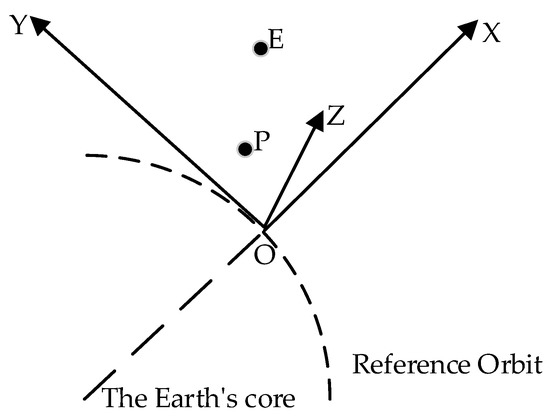
Figure 1.
The local-vertical local-horizontal (LVLH) coordinate system.
The C–W equations can be expressed as
where P and E represent the pursuer and the evader, respectively. ω represents the orbital angular velocity of the origin O. xi, , and represent the position components of the players in the relative coordinate system. , , and , respectively, represent control variables in the three directions (i.e., x, y, and z axis).
The state variables of both players are represented by as follows:
Thus, the dynamics equations can be written as
where
is the control variable, which satisfies . and are constants.
Furthermore, we take the relative states of the two spacecraft as state variables. By defining , the state equations are converted to
where .
By taking the terminal distance as the cost, the objective function can be defined as
where .
3. Construction of Guaranteed Cost Strategy with Perfect Information
To solve the orbital pursuit-evasion problem given in the second section and enable the players to achieve their individual goals, we should construct a feedback control for the players. However, for the orbital pursuit-evasion problem with bounded control, it is difficult to get optimal feedback control by solving the HJI equation. Therefore, researchers have focused on constructing near-optimal feedback control. The existing near-optimal feedback control strategies [15,16] are based on solving numerous open-loop solutions, which is time-consuming and cannot guarantee capture.
To overcome this shortcoming, we derive a guaranteed cost strategy by adopting the Lyapunov-like function-based method [17] and the matrix analysis theory. Besides, we propose a hybrid method combining the homotopy method and Newton’s method to calculate the unknown time-to-go in this strategy. This guaranteed cost strategy can guarantee the miss distance and does not need to solve numerous open-loop solutions. The detailed procedure is shown as follows.
3.1. The Guaranteed Cost Strategy
For the sake of brevity, we define the zero-effort-miss (ZEM) variables as follows:
where is the zero-input state transfer matrix of Equation (5) and satisfies .
Substituting Equation (7) into Equations (5) and (6), the system is reduced to
where , .
Define the Lyapunov-like function , . Thus, the change rate of over time satisfies
where .
The feedback control strategies of the pursuer and the evader can be obtained by minimizing or maximizing the change rate:
where and are the upper boundaries of the control of the pursuer and the evader, respectively. The time-to-go is an unknown variable and needs to be calculated in real time. The feedback control strategies can guarantee the cost (i.e., miss distance) for the pursuer and the evader when the time-to-go is appropriate. The feedback control strategies with appropriate time-to-go are called guaranteed cost strategies.
When the pursuer adopts , its corresponding time-to-go can be obtained by substituting into Equation (9) to obtain
As is derived by maximizing the change rate (9), we get
As , according to the matrix analysis theory, we get
where and , respectively, represent the maximum and minimum eigenvalues of the matrix .
Thus, Equation (12) can be further expressed as
Integrate Equation (14) to obtain
From Equation (15), it is seen that when the pursuer adopts , the cost (i.e., miss distance) will not exceed the value . If the safe distance between the players is m, we can calculate the time-to-go by solving the equation . Thus, when the pursuer adopts , the capture of the evader can be guaranteed within .
Similarly, we get
From Equation (16), it is seen that when the evader adopts , the cost (i.e., miss distance) is not less than the value . Then, we can calculate the time-to-go by solving the equation . Due to the control constraint , the evader cannot avoid being captured when the pursuer chooses the appropriate strategy. However, when the evader adopts , it can escape from the pursuer before .
3.2. Time-To-Go Calculation
For the sake of brevity, define the range , where is the orbital angular velocity of the origin of the LVLH coordinate system. The equation is converted to
Similarly, define . The equation is converted to
We can get the appropriate time-to-go by solving Equations (17) and (18). However, the analytic solution of the equations is difficult to obtain since the equations are nonlinear. Thus, we use the numerical method to solve the equations. The iterative method is an effective numerical method for solving nonlinear equations. However, most iterative methods (such as Newton’s method) require appropriate initial guesses. If the initial value is not selected properly, it is difficult to obtain the solution of the nonlinear equation. Unfortunately, the appropriate initial values for Equations (17) and (18) are difficult to find. Define functions and as follows:
Figure 2 shows the shapes of functions and in Equation (19) with different current states. The different current relative states for four cases are shown in Table 1. The functions’ shapes are highly dependent on the current states, and their uncertainty makes it difficult to find an appropriate initial value. As noted by Yamamura [28], the homotopy method is good at global convergence. Thus, using the homotopy method to calculate the time-to-go can avoid the convergence problem caused by the improper selection of initial value. However, the homotopy method is not good at convergence speed. Thus, we propose a hybrid method combining the homotopy method and Newton’s method to calculate the time-to-go.
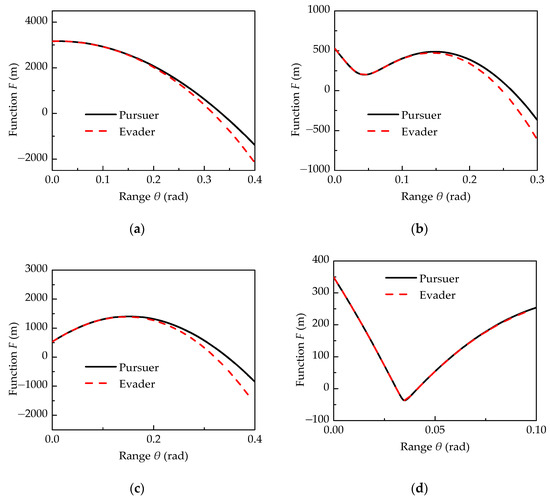
Figure 2.
The function F change with range θ in (a) case 1, (b) case 2, (c) case 3 and (d) case 4.

Table 1.
Current relative states of different cases.
3.2.1. Time-To-Go Calculation Based on the Homotopy Method
For the sake of brevity, ignore the superscripts and subscripts, and use F for the functions and , and for the variables and . To solve the nonlinear equation , we construct the fixed-point homotopy equation as follows:
where . The solution of is the desired solution, whereas the solution of is , which can be any specified value. As shown in Figure 3, when the variable p increases from 0 to 1, the solution of the homotopy equation changes continuously from to the expected solution along the homotopy path. The detailed procedure is shown as follows.
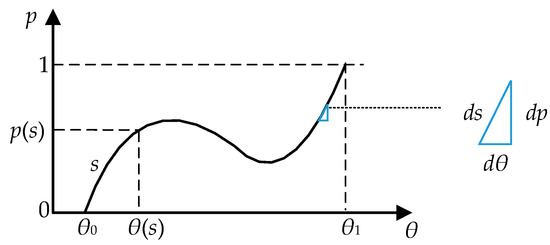
Figure 3.
The homotopy curve.
To find the solution along the homotopy path, first, we need to get the unit tangent vector of the homotopy path. Let and , where s is the arc length along the homotopy path. The derivative of with respect to s is
where
Considering the arc length constraint, the relationship between , p, and s is as follows:
The unit tangent vector of the homotopy path can be obtained by combining Equations (21) and (23):
where , .
By integrating the unit tangent vector until p = 1 is satisfied, the desired solution can be obtained. The iterative equation is as follows:
where h is the step length.
To meet the accuracy requirements of the solution, a correction method is used after each iteration step of Equation (25). The correction equation is as follows:
Repeat Equation (26) until is brought beneath the desired value.
3.2.2. Time-to-Go Calculation Based on the Hybrid Method
Although the homotopy method is good at global convergence, it is not good at convergence speed. In many cases (when the initial value is appropriate), Newton’s method can also achieve good convergence. Thus, we propose a hybrid method combining the homotopy method and Newton’s method, which takes into account the validity and rapidity of the algorithm. The specific steps are given as follows:
- Step1. Take the time-to-go calculated at the last moment in the confrontation as the initial value at the current moment.
- Step2. Set the maximum iteration number N, and calculate the time-to-go using Newton’s method, i.e., . If convergence can be obtained within the maximum iteration number, the operation will end and the time-to-go will be obtained. Otherwise, go to step 3.
- Step3. Calculate the time-to-go by using the homotopy method. Use Equation (25) for calculation and Equation (26) for correction. Repeat the iteration until p = 1 is satisfied, and the time-to-go is obtained.
Since we use the time-to-go of the previous step as the initial guess value of the current step, the initial value is appropriate in most cases. The time-to-go of the current step can be found quickly by using Newton’s method, which is second-order convergence. The homotopy method will be used only at the beginning moment or at a few special moments when the time-to-go suddenly changes (as shown in Examples 2 and 3), and the convergence speed is relatively slower.
It should be noted that the time-to-go calculation using the hybrid method is based on the premise that the range and bearings of the spacecraft are measurable. In the case of bearings-only measurements, the time-to-go cannot be calculated by this method.
4. Compensation Control Strategy for Delayed Information
In this section, we present a compensation method for the time delay caused by the measurement and estimation process. By adopting this method to modify the guaranteed cost strategies given in the third section, we get the compensation control strategies.
4.1. Time Delay Compensation Method Based on Uncertainty Set
Few works have yet dealt with the orbital pursuit-evasion problem with delay information. However, several works on delay information have been done in other areas. To compensate for the delay information in the pursuit-evasion problem, Petrosjan [18] proposed the reachability set (uncertainty set) method and proved that the optimal strategy of the pursuer is the pursuit of the center of the reachability set of the evader. References [19,20,21,22,23,24,25] applied this method for missile guidance, which partially compensates for the information delay and effectively improves the guidance accuracy.
However, the above works assumed two-dimensional situations, partial delay, and no gravity difference. These assumptions are invalid in the orbital pursuit-evasion problem. Thus, without the consideration of these assumptions, the calculation of the uncertainty set is more complicated. To get the geometric center of the spacecraft’s uncertainty set, we analyze the uncertain set’s characteristics based on the linear system theory rather than calculate the uncertainty set. Then, the delayed state is replaced by the uncertainty set’s center. The detailed procedure is shown as follows.
First, we give a definition of the uncertainty set. In the case delay time , the player’s current state value is unknown to the opponent. The opponent can calculate the set of all possible state values based on the delayed state information he gets and the player’s control constraint. This set is called the uncertainty set (denoted by S).
Ignoring the subscripts, the spacecraft dynamics (3) can be expressed as follows:
where .
Let be the delay period. According to the linear system theory [29], the terminal state satisfies
According to the definition of the uncertainty set, for any given , there exists a corresponding control strategy , which satisfies such that
Let , where . The terminal state corresponding to can be expressed as
According to the definition of the uncertainty set, we have . Combining Equations (29) and (30) yields
Equation (30) can be further expressed as
According to Equation (32), states and are centrally symmetric about point in the state space.
Thus, we have the following conclusion: In the system described by Equation (27), for any given , there exists a corresponding state such that and are centrally symmetric about point in the state space.
Besides, the spacecraft’s control is bounded. Thus, the total energy it can provide over delay time is limited. Under the condition of finite energy and fixed time, the spacecraft’s reachable state is limited, which means the uncertainty set is a bounded set.
According to the above analysis, the uncertainty set’s geometric center is
The delay information can be compensated by replacing the state variable with the center of the uncertainty set.
4.2. Compensation Control Strategy
In this part, by modifying the guaranteed cost strategy through the above time delay compensation method, we obtain the compensation control strategy for the time delay scenario. Due to the existence of delay time , the information obtained at time t is the opponent’s state information at time . Although the opponent’s state information at time t is not known, the uncertainty set can be calculated. Then the center of the uncertainty set is taken as the opponent’s estimation state at time t. The compensation control strategies are given as follows:
where , . is the estimated relative state after compensation.
5. State Estimation Based on UKF
Before applying the compensation control strategies given in the above section to the orbital pursuit-evasion problem, the spacecraft’s state needs to be measured. However, noise is included in the measured data. To determine the opponent’s state, we need to estimate the state of the spacecraft based on the observed data. Radar is a relative measurement sensor commonly used in space missions. We use radar as the measurement sensor. Besides, since the measurement equation is nonlinear, we need to adopt a nonlinear filtering method. Nonlinear filtering methods mainly include the extended Kalman filter (EKF), UKF, and particles filter (PF) [30]. Compared with PF, UKF has lower computational complexity [31]. Compared with EKF, UKF has better performance [31]. Thus, we use UKF to estimate the state. In this section, the spacecraft state estimation model is first established, and then the UKF toolkit [32] is used to estimate the spacecraft state.
The spacecraft motion equation with environmental perturbation can be expressed as follows:
where is the equivalent noise of environmental perturbation, which follows the normal distribution , , , .
We use radar as the measurement sensor. Taking relative distance , elevation angle , and azimuth angle as measurement variables, the measurement equation can be expressed as follows:
where V is the measurement noise, which follows the normal distribution.
Before UKF is used for state estimation, the continuous system needs to be discretized. We use the solution formula of the state equation to ensure that the continuous state equation and the discrete state equation have the same solution at the sampling point. The discretized system equation is as follows:
where , , , .
Finally, the UKF toolkit [32] is used to estimate the spacecraft state based on the established model.
6. Results and Discussion
To verify the effectiveness of the proposed method, we present several numerical simulations. The simulation is divided into the following two parts. The first part is to verify the effectiveness of the guaranteed cost strategy proposed in this paper. The second part is to verify the effectiveness of the compensation control strategy by comparing the orbital pursuit-evasion problem under three scenarios: no time delay, with compensation for time delay, and without compensation for time delay.
In these simulations, the initial altitude of the reference orbit is 500 km, the control boundary of the pursuer is , the control boundary of the evader is , the safe distance between the players is , and the sampling step is 0.01 s. The initial state of the pursuer and the evader is shown in Table 2.
Table 2.
Positions and velocities of the initial time.
6.1. Examples of Guaranteed Cost Strategy
To verify the guaranteed cost strategy’s effectiveness, we give the following example without considering noise and time delay.
Example 1.
Both pursuer and evader adopt the guaranteed cost strategy.
Figure 4 shows the positions changing with time during the confrontation. From Figure 4, it can be seen that the pursuer finally intercepts the evader, and the interception time is 209.56 s. The terminal miss distance is 0.9013 m, which is less than the safe distance.
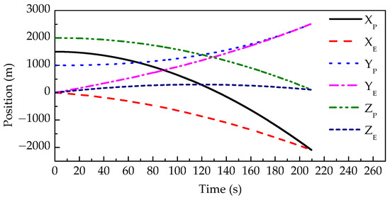
Figure 4.
The position of each player changing with time.
Figure 5 shows and () changing with time during the confrontation. As shown in Figure 5a, at the beginning of the confrontation, the pursuer’s time-to-go is 212.27 s, and the evader’s time-to-go is 207.75 s. This result means the pursuer can guarantee capture within 212.27 s, and the evader can avoid capture within 207.75 s by adopting the guaranteed cost strategies. As shown in Figure 5b, decreases with time and turns to zero at the end of the confrontation. This result means and approach the real interception time as time goes on.
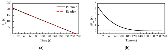
Figure 5.
(a) tgo and (b) Δtgo changing with time.
Figure 6 shows the control variable changing with time during the confrontation. In this figure, the pursuer’s control is similar to the evader’s control. The reason is that is close to during the confrontation.
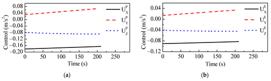
Figure 6.
The control variable of (a) the pursuer and (b) the evader changing with time.
In the case of , when the pursuer chooses the appropriate control strategy, the pursuer will eventually capture the evader no matter how the evader reacts. However, the guaranteed cost strategy provides an opportunity to determine upper and lower bounds on the capture time. When the evader chooses the guarantee cost strategy, the capture time can be guaranteed to be greater than . When the pursuer chooses the guarantee cost strategy, the capture time can be guaranteed to be less than .
As can be seen from the above example, the evader is intercepted by the pursuer in 209.56 s, which is less than 212.27 s () and greater than 207.75 s (). The effectiveness of the guaranteed cost strategy is verified. By adopting the guaranteed cost strategy, the pursuer can guarantee capture within , and the evader can avoid capture before .
6.2. Examples of Compensation Control Strategy
To verify the effectiveness of the compensation control strategy proposed in this paper, we compare the orbital pursuit-evasion problem under three scenarios: no time delay, with compensation for time delay, and without compensation for time delay. Consider the following two examples: the first example is that the evader’s information has no time delay, and the pursuer plays under the above three scenarios. The second example is that the pursuer’s information has no time delay, and the evader plays under the above three scenarios. The covariance of the process noise is set as , and the covariance of the measurement noise is set as . We present a Monte Carlo simulation for each case.
Example 2.
The evader’s information has no time delay, and the pursuer plays under three scenarios: no time delay, with compensation for time delay, and without compensation for time delay. The delay time is 1 s.
- (1)
- Terminal Time is Free
Figure 7 shows the estimation errors of the relative state. From Figure 7, it can be seen that the estimation errors in relative position are about the order of magnitude 1 × 10⁻⁵ m, and the estimation errors in relative velocity are about the order of magnitude 1 × 10⁻³ m/s.
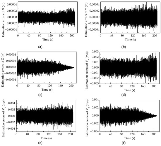
Figure 7.
The estimation errors of the relative state: (a) X, (b) Y, (c) Z, (d) VX, (e) VY, and (f) VZ.
Figure 8 shows the average relative distance of 100 Monte Carlo runs between the players in three scenarios: the pursuer plays without time delay, without compensation for time delay, and with compensation for time delay. When the pursuer plays without time delay, the average interception time is 209.56 s. The average terminal distance between the two players is 0.9013 m, which is less than the safe distance. When the pursuer plays without compensation for time delay, the average relative distance between the two players reaches the minimum value of 19.1841 m at 206.89 s. After that, the relative distance increases. The reason is that after a period of acceleration, the velocity has reached a relatively large value. After the two players miss each other, it takes a while for the velocity to change. However, the distance between the players still increases, which means the pursuer cannot intercept the evader in a short time. When the pursuer plays with compensation for time delay, the average interception time is 211.69 s. The average terminal distance between the two spacecraft is 0.9763 m, which is less than the safe distance. By comparison, we can see that with compensation for time delay, the pursuer can significantly reduce the relative distance between the pursuer and the evader. Although the interception time is longer than that in the no time delay scenario, it still intercepts the evader successfully.
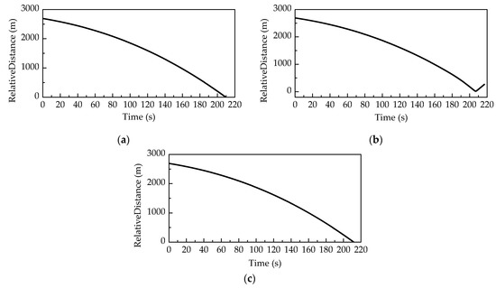
Figure 8.
The average relative distance of 100 Monte Carlo runs in the scenario that the pursuer plays (a) without time delay; (b) without compensation for time delay; and (c) with compensation for time delay.
Figure 9 shows the average and of 100 Monte Carlo runs between the players in three scenarios: the pursuer plays without time delay, without compensation for time delay, and with compensation for time delay. When the pursuer plays without time delay, decreases linearly with time, is a non-negative value during the confrontation. When the pursuer plays without compensation for time delay, the evader’s time-to-go suddenly increases at 177.76 s, which means the evader can avoid capture for a longer time. This phenomenon is caused by a change in the system state. The pursuer’s control deviates from the guaranteed cost strategy due to delayed information, which leads to the system state deviating from the expected trajectory. It thus gives the evader a chance to prolong the interception time. However, the pursuer’s time-to-go does not increase until 206.61 s. The reason is that the pursuer’s delayed information misleads the calculation of . When the pursuer plays with compensation for time delay, the time-to-go corresponding to the pursuer and the evader slightly deviates from that of the no delay scenario. The reason is that the compensation method cannot completely eliminate the effect of delayed information.
Figure 9.
The average tgo and Δtgo of 100 Monte Carlo runs in the scenario that the pursuer plays (a) without time delay; (b) without compensation for time delay; and (c) with compensation for time delay.
Figure 10 shows the average control variable of 100 Monte Carlo runs between the players in three scenarios: the pursuer plays without time delay, without compensation for time delay, and with compensation for time delay. When the pursuer plays without time delay, the control trajectories are linear during the confrontation. When the pursuer plays without compensation for time delay, the evader’s control switches at 177.76 s. This phenomenon is caused by a sudden change in . The pursuer’s control decreases from 178.77 s due to the state change caused by the evader’s control switch. The pursuer’s control switches at 206.61 s due to the sudden change in . When the pursuer plays with compensation for time delay, the pursuer’s control and the evader’s control slightly deviate from the no-delay ones due to the delayed information.
Figure 10.
The average control variable of 100 Monte Carlo runs in the scenario that the pursuer plays (a) without time delay; (b) without compensation for time delay; and (c) with compensation for time delay.
- (2)
- Terminal Time is Fixed
The terminal time is set as 212 s.
Figure 11 shows the average ZEM distance of 100 Monte Carlo runs in three fixed-time scenarios: the pursuer plays without time delay, without compensation for time delay, and with compensation for time delay. When the pursuer plays without time delay, the average terminal distance between the two players reaches 0.00003202 m, which is less than the safe distance. When the pursuer plays without compensation for time delay, the average terminal distance between the two players is 25.6273 m, which means the pursuer failed to intercept the evader. When the pursuer plays with compensation for time delay, the average terminal distance between the two players reaches 0.1064 m, which is less than the safe distance. According to Figure 11b, when the pursuer has delayed information, the zero-effort miss distance at the beginning of the confrontation shows an upward trend. The reason is that the pursuer adopts no control at the beginning of the confrontation due to lack of information. According to Figure 11c, when the pursuer plays without time delay, the average zero-effort miss distance reaches below the safe distance at 180.43 s. When the pursuer plays with compensation for time delay, the average zero-effort miss distance reaches below the safe distance at 202.59 s. However, when the pursuer plays without compensation for time delay, the zero-effort miss distance converges to a large value, which means the pursuer cannot intercept the evader.
Figure 11.
The average ZEM distance of 100 Monte Carlo runs: (a) the ZEM distance changing with time; zoom in on the curve at (b) the beginning of the confrontation and (c) the end of the confrontation.
Example 3.
The pursuer’s information has no time delay, and the evader plays under three scenarios: no time delay, with compensation for time delay, and without compensation for time delay. The delay time is 1 s.
- (3)
- Terminal Time is Free
Figure 12 shows the average relative distance of 100 Monte Carlo runs between the players in three scenarios: the evader plays without time delay, without compensation for time delay, and with compensation for time delay. When the evader plays without time delay, the average interception time is 209.56 s. The average terminal distance between the two players is 0.9013 m, which is less than the safe distance. When the evader plays without compensation for time delay, the average interception time is 204.39 s. The average terminal distance between the two players is 0.7960 m, which is less than the safe distance. When the evader plays with compensation for time delay, the average interception time is 208.48 s. The average terminal distance between the two spacecraft is 0.9904 m, which is less than the safe distance. By comparison, we can see that the pursuer can successfully intercept the evader in all scenarios. In the time delay scenarios, the interception time is shorter than that in the no-delay scenario. The reason is that the pursuer takes advantage of the evader’s control based on delay information to shorten the interception time in the time delay scenarios. The interception time in the scenario that the evader plays without compensation for time delay is shorter than that in the scenario the evader plays with compensation for time delay, which means the compensation control strategy can help the evader prolong the interception time.
Figure 12.
The average relative distance of 100 Monte Carlo runs in the scenario that the evader plays (a) without time delay; (b) without compensation for time delay; and (c) with compensation for time delay.
Figure 13 shows the average and of 100 Monte Carlo runs between the players in three scenarios: the evader plays without time delay, without compensation for time delay, and with compensation for time delay. When the evader plays without time delay, decreases linearly with time, and is a non-negative value during the confrontation. When the evader plays without compensation for time delay, the evader’s time-to-go suddenly increases at 176.43 s. The reason is that the evader’s delayed information misleads the calculation of . When the evader plays with compensation for time delay, the time-to-go corresponding to the pursuer and the evader slightly deviates from that of the no-delay scenario. The reason is that the compensation method cannot completely eliminate the effect of delayed information.
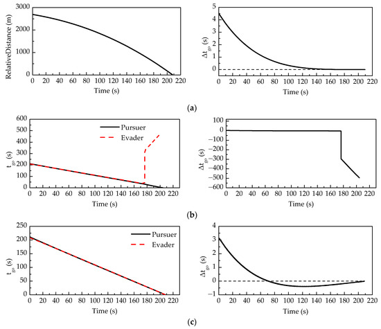
Figure 13.
The average tgo and Δtgo of 100 Monte Carlo runs in the scenario that the evader plays (a) without time delay; (b) without compensation for time delay; and (c) with compensation for time delay.
Figure 14 shows the average control variable of 100 Monte Carlo runs between the players in three scenarios: the evader plays without time delay, without compensation for time delay, and with compensation for time delay. When the evader plays without time delay, the control trajectories are linear during the confrontation. When the evader plays without compensation for time delay, its control switches at 176.43 s. This phenomenon is caused by a sudden change in . The evader’s control deviates from the guaranteed cost strategy due to the delayed information, which leads to the system state deviating from the expected trajectory. It thus gives the pursuer a chance to shorten the interception time. The pursuer’s control decreases from 176.44 s due to the state change caused by the evader’s control switch. When the evader plays with compensation for time delay, the pursuer’s control and the evader’s control slightly deviate from the no-delay ones due to the delayed information.
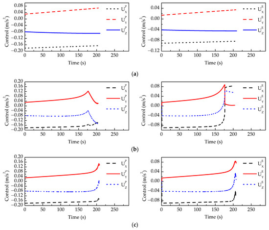
Figure 14.
The average control variable of 100 Monte Carlo runs in the scenario that the evader plays (a) without time delay; (b) without compensation for time delay; and (c) with compensation for time delay.
- (4)
- Terminal Time is Fixed
The terminal time is set as 212 s.
Figure 15 shows the average ZEM distance of Monte Carlo runs in three fixed-time scenarios: the evader plays without time delay, without compensation for time delay, and with compensation for time delay. When the evader plays without time delay, the average terminal distance between the two players reaches 0.00005056 m, which is less than the safe distance. When the evader plays without compensation for time delay, the average terminal distance between the two players reaches 0.00005425 m, which is less than the safe distance. When the evader plays with compensation for time delay, the terminal distance between the two players reaches 0.00004705 m, which is less than the safe distance. According to Figure 15b, when the evader has delayed information, the zero-effort miss distance at the beginning of the confrontation declines faster than that in the no-delay scenario. The reason is that the evader adopts no control at the beginning of the confrontation due to the lack of information. At the terminal time, the pursuer can successfully intercept the evader in all scenarios, and the terminal distances are close to each other.
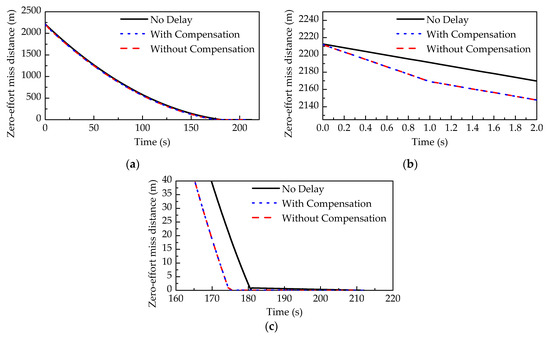
Figure 15.
The average ZEM distance of 100 Monte Carlo runs: (a) the ZEM distance changing with time; zoom in on the curve at (b) the beginning of the confrontation and (c) the end of the confrontation.
Example 2 shows that when the pursuer has delayed information, the compensation control strategy proposed in this paper can shorten the relative distance between the players and increase the possibility of intercepting the evader. Example 3 shows that when the evader has delayed information, the compensation control strategy proposed in this paper prolongs the time that the pursuer takes to intercept the evader.
7. Conclusions
In this paper, we derive a guaranteed cost strategy based on a Lyapunov-like function and matrix analysis theory, and propose a time delay compensation method for the orbital pursuit-evasion problem based on the uncertainty set. By combining the time delay compensation method with the guaranteed cost strategy, we derive a compensation control strategy.
The simulation results show the following:
- The proposed guaranteed cost strategy is valid in the orbital pursuit-evasion problem with perfect information. By adopting the guaranteed cost strategy, the pursuer can guarantee capture within , and the evader can avoid capture before .
- The proposed compensation control strategy is applicable to the orbital pursuit-evasion problem with imperfect information. When the pursuer has imperfect information, the compensation control strategy can shorten the relative distance between the players and increase the possibility of intercepting the evader. When the evader has imperfect information, the compensation control strategy can prolong the time that the pursuer takes to intercept the evader.
Author Contributions
Conceptualization, J.Z. and L.Z.; methodology, J.Z., H.L., and J.C.; formal analysis, H.L.; investigation, S.W.; writing—original draft preparation, J.Z.; writing—review and editing, J.Z. and S.W. All authors have read and agreed to the published version of the manuscript.
Funding
This research was funded by the National Natural Science Foundation of China (Nos. 61633008, 61773132, 61803115).
Institutional Review Board Statement
Not applicable.
Informed Consent Statement
Not applicable.
Data Availability Statement
The data presented in this study are contained in the article itself.
Conflicts of Interest
The authors declare no conflict of interest.
References
- Jagat, A.; Sinclair, A.J. Optimization of spacecraft pursuit-evasion game trajectories in the euler-hill reference frame. In Proceedings of the AIAA/AAS Astrodynamics Specialist Conference, San Diego, CA, USA, 4–7 August 2014; p. 4131. [Google Scholar]
- Stupik, J. Optimal Pursuit/Evasion Spacecraft Trajectories in the Hill Reference Frame. Master’s Thesis, University of Illinois at Urbana-Champaign, Urbana, IL, USA, 2013. [Google Scholar]
- Ye, D.; Shi, M.; Sun, Z. Satellite proximate pursuit-evasion game with different thrust configurations. Aerosp. Sci. Technol. 2020, 99, 105715. [Google Scholar] [CrossRef]
- Zhou, J.; Zhao, L.; Cheng, J.; Wang, S.; Wang, Y. Pursuer’s Control Strategy for Orbital Pursuit-Evasion-Defense Game with Continuous Low Thrust Propulsion. Appl. Sci. 2019, 9, 3190. [Google Scholar] [CrossRef]
- Pontani, M.; Conway, B.A. Numerical solution of the three-dimensional orbital pursuit-evasion game. J. Guid. Control Dyn. 2009, 32, 474–487. [Google Scholar] [CrossRef]
- Woodbury, T.D.; Hurtado, J.E. Adaptive play via estimation in uncertain nonzero-sum orbital pursuit evasion games. In Proceedings of the AIAA SPACE and Astronautics Forum and Exposition, Orlando, FL, USA, 12–14 September 2017; p. 5247. [Google Scholar]
- Linville, D.; Hess, J. Linear Regression Models Applied to Spacecraft Imperfect Information Pursuit-Evasion Differential Games. In Proceedings of the AIAA Scitech 2020 Forum, Orlando, FL, USA, 6–10 January 2020. [Google Scholar]
- Pontani, M. Numerical solution of orbital combat games involving missiles and spacecraft. Dyn. Games Appl. 2011, 1, 534–557. [Google Scholar] [CrossRef]
- Basar, T.; Olsder, G.J. Dynamic Noncooperative Game Theory; Society for Industrial and Applied Mathematics: Philadelphia, PA, USA, 1999. [Google Scholar]
- Sun, S.T.; Zhang, Q.H.; Chen, Y. Numerical solution for a class of pursuit-evasion problem in low earth orbit. In Proceedings of the 9th Asian Control Conference, Istanbul, Turkey, 23–26 June 2013; pp. 1–6. [Google Scholar]
- Hafer, W.T.; Reed, H.L.; Turner, J.D.; Pham, K. Sensitivity methods applied to orbital pursuit evasion. J. Guid. Control Dyn. 2015, 38, 1118–1126. [Google Scholar] [CrossRef]
- Sun, S.T.; Zhang, Q.H.; Loxton, R.; Li, B. Numerical solution of a pursuit-evasion differential game involving two spacecraft in low earth orbit. J. Ind. Manag. Optim. 2015, 11, 1127–1147. [Google Scholar] [CrossRef]
- Shen, H.X.; Casalino, L. Revisit of the three-dimensional orbital pursuit-evasion game. J. Guid. Control Dyn. 2018, 41, 1823–1831. [Google Scholar] [CrossRef]
- Li, Z.Y.; Zhu, H.; Yang, Z.; Luo, Y.Z. A dimension-reduction solution of free-time differential games for spacecraft pursuit-evasion. Acta Astronaut. 2019, 163, 201–210. [Google Scholar] [CrossRef]
- Ghosh, P.; Conway, B.A. Near-optimal feedback strategies synthesized using a spatial statistical approach. J. Guid. Control Dyn. 2013, 36, 905–919. [Google Scholar] [CrossRef]
- Anderson, G.M. Feedback control for a pursuing spacecraft using differential dynamic programming. AIAA J. 1977, 15, 1084–1088. [Google Scholar] [CrossRef]
- Gutman, S. On Optimal Guidance for Homing Missiles. J. Guid. Control Dyn. 1979, 2, 296–300. [Google Scholar] [CrossRef]
- Petrosjan, L.A. Differential Games of Pursuit; World Scientific: Singapore, 1993. [Google Scholar]
- Kumkov, S.; Patsko, V. Optimal strategies in a pursuit problem with incomplete information. J. Appl. Math. Mech. 1995, 59, 75–85. [Google Scholar] [CrossRef]
- Shinar, J.; Glizer, V.Y. Solution of a delayed information linear pursuit-evasion game with bounded controls. Int. Game Theory Rev. 1999, 1, 197–217. [Google Scholar] [CrossRef]
- Shinar, J.; Shima, T.; Glizer, V.Y. On the compensation of imperfect information in dynamic games. Int. Game Theory Rev. 2000, 2, 229–248. [Google Scholar] [CrossRef]
- Shinar, J.; Shima, T. Nonorthodox guidance law development approach for intercepting maneuvering targets. J. Guid. Control Dyn. 2002, 25, 658–666. [Google Scholar] [CrossRef]
- Shinar, J.; Glizer, V.Y. New Approach to Improve the Accuracy in Delayed Information Pursuit-Evasion Games; Birkhäuser Boston: Boston, MA, USA, 2006. [Google Scholar]
- Glizer, V.Y.; Turetsky, V. A linear differential game with bounded controls and two information delays. Optim. Control Appl. Methods 2009, 30, 135–161. [Google Scholar] [CrossRef]
- Glizer, V.Y.; Turetsky, V.; Shinar, J. Differential game with linear dynamics and multiple information delays. In Proceedings of the 13th WSEAS International Conference on Systems, Stevens Point, WI, USA, 22–24 July 2009; pp. 179–184. [Google Scholar]
- Clohessy, W.H.; Wiltshire, R.S. Terminal guidance system for satellite rendezvous. J. Aerosp. Sci. 1960, 27, 653–658. [Google Scholar] [CrossRef]
- Shepperd, S.W. Constant covariance in local vertical coordinates for near-circular orbits. J. Guid. Control Dyn. 1991, 14, 1318–1322. [Google Scholar] [CrossRef]
- Yamamura, K.; Arai, K.; Kiyoi, M. A piecewise-linear homotopy method for nonlinear programming. Electron. Commun. Jpn. 1991, 74, 28–38. [Google Scholar] [CrossRef]
- Chen, C.T. Linear System Theory and Design; Oxford University Press: New York, NY, USA, 1999. [Google Scholar]
- Li, G.; Sun, F.; Cheng, N. Performance analysis of UKF for nonlinear problems. In Proceedings of the 2009 Third International Symposium on Intelligent Information Technology Application, Nanchang, China, 21–22 November 2009; pp. 209–212. [Google Scholar]
- Farina, A.; Ristic, B.; Benvenuti, D. Tracking a ballistic target: Comparison of several nonlinear filters. IEEE Trans. Aerosp. Electron. Syst. 2002, 38, 854–867. [Google Scholar] [CrossRef]
- Särkkä, S.; Hartikainen, J.; Solin, A. EKF/UKF Toolbox for Matlab V1.3; Aalto University School of Sciency: Espoo, Finland, 2011. [Google Scholar]
Publisher’s Note: MDPI stays neutral with regard to jurisdictional claims in published maps and institutional affiliations. |
© 2021 by the authors. Licensee MDPI, Basel, Switzerland. This article is an open access article distributed under the terms and conditions of the Creative Commons Attribution (CC BY) license (http://creativecommons.org/licenses/by/4.0/).