
Improving the Accuracy of Analytical Relationships for Mechanical Properties of Permeable Metamaterials


Abstract
1. Introduction
2. Materials and Methods
2.1. Euler–Bernoulli Beam Theory
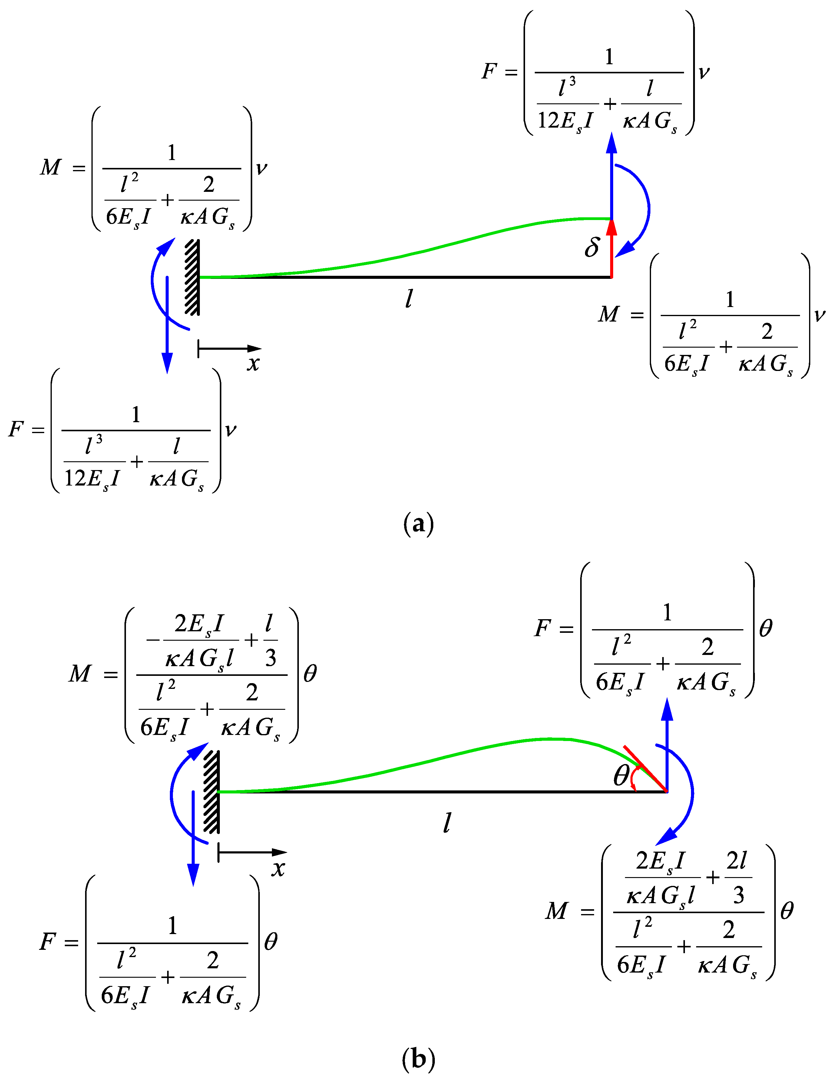
2.2. Timoshenko Beam Theory
2.3. From Euler–Bernoulli to Timoshenko
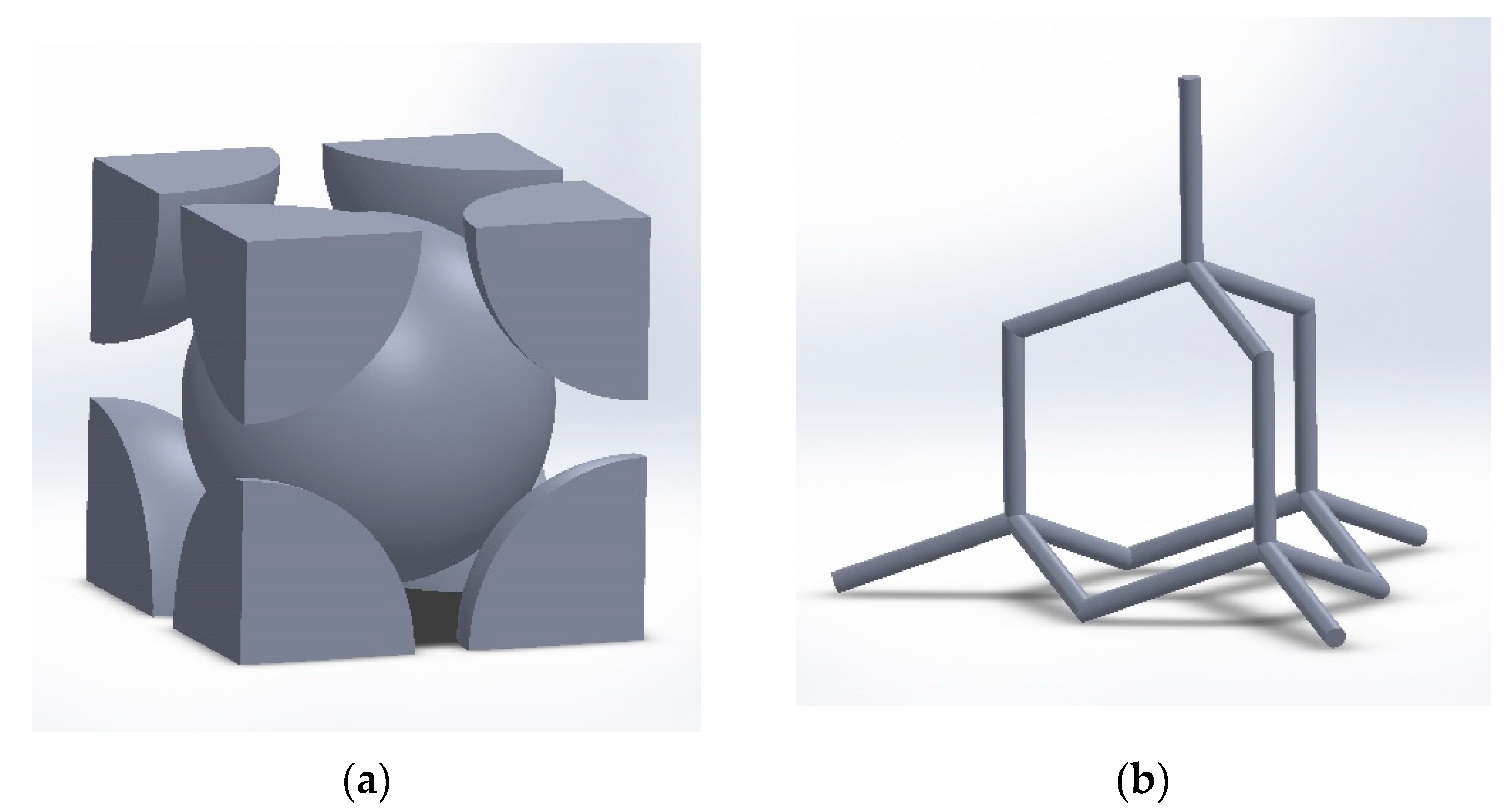
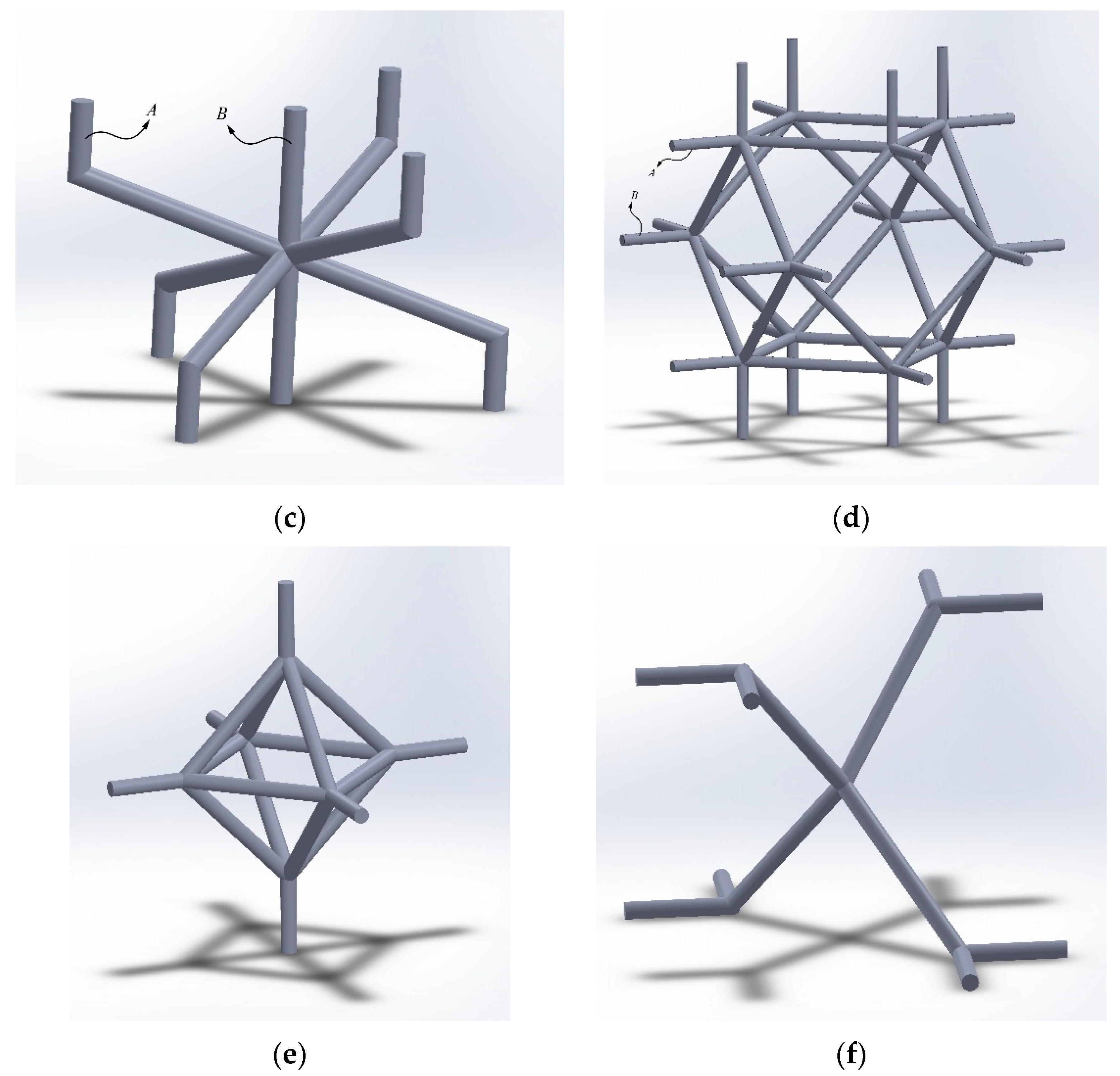
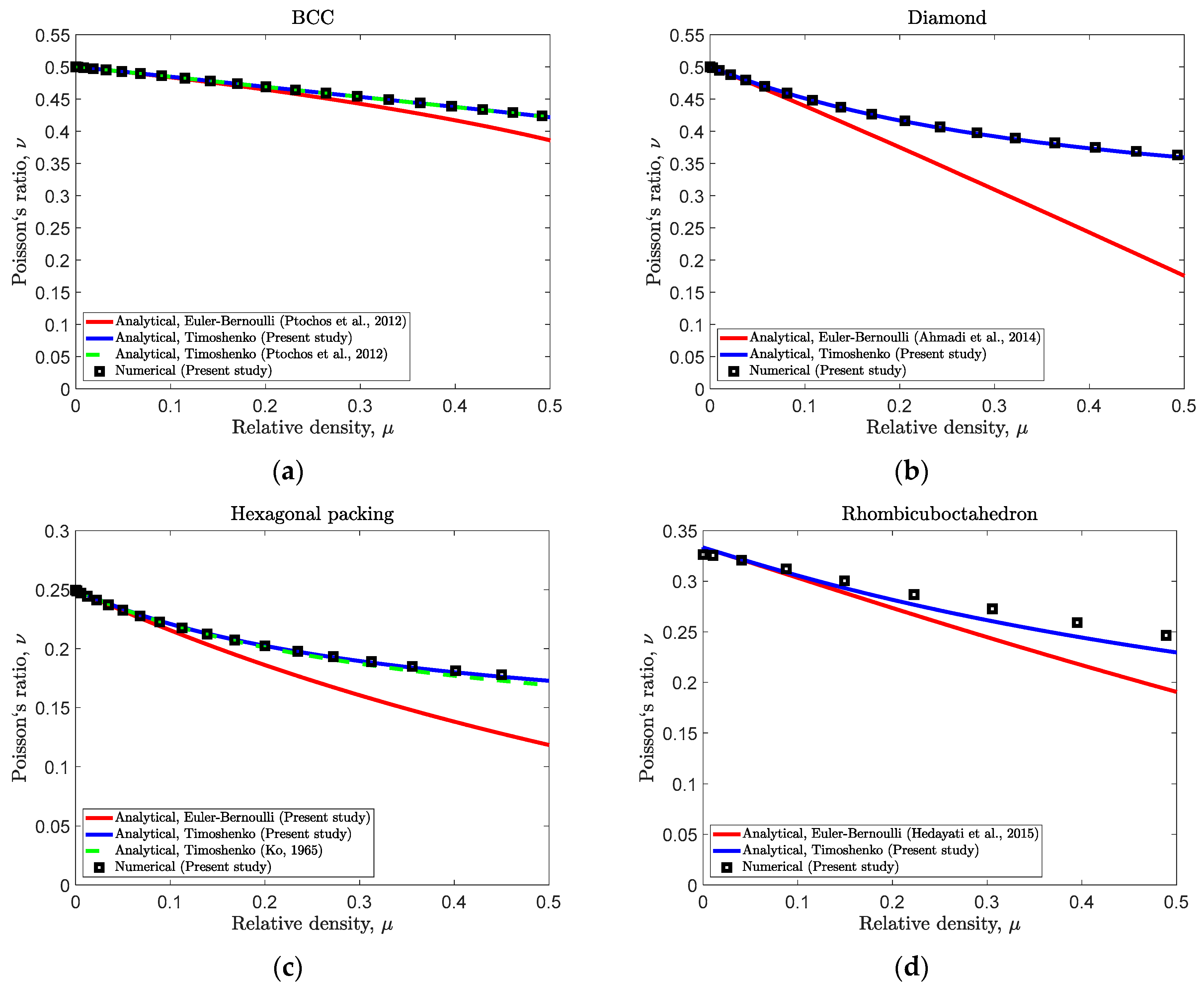
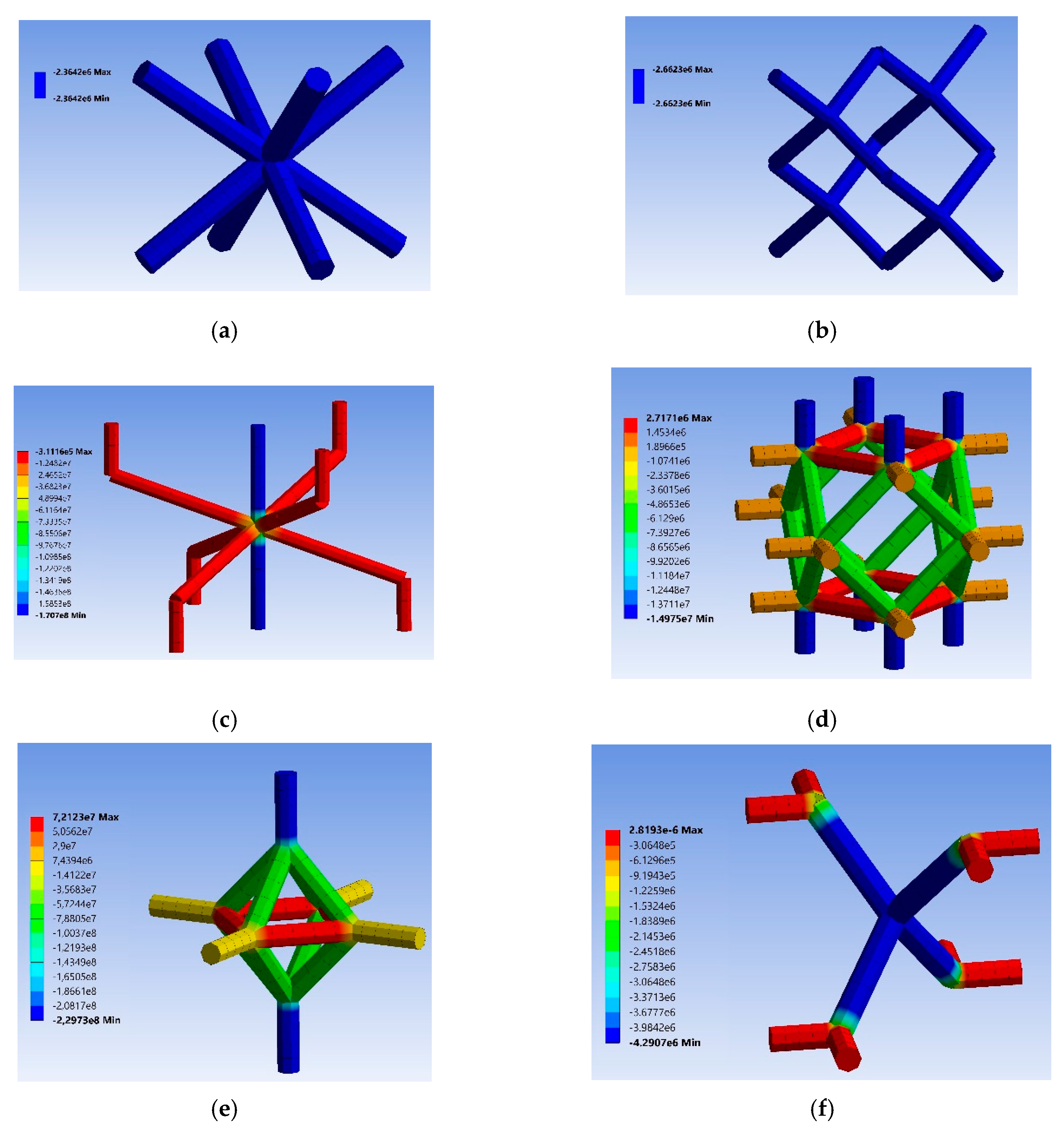
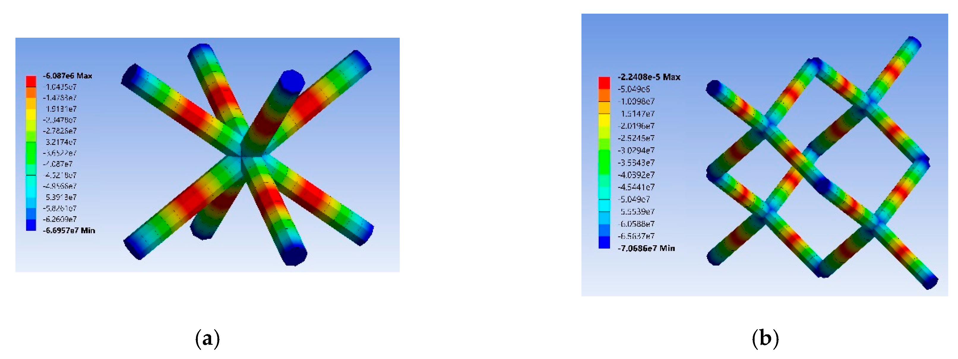
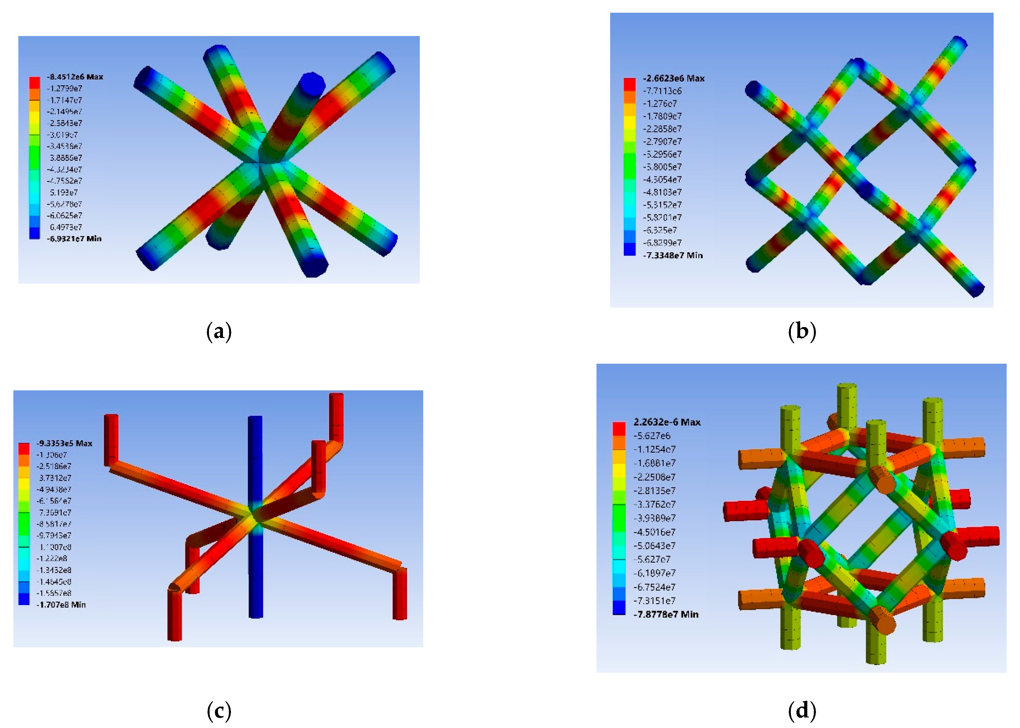
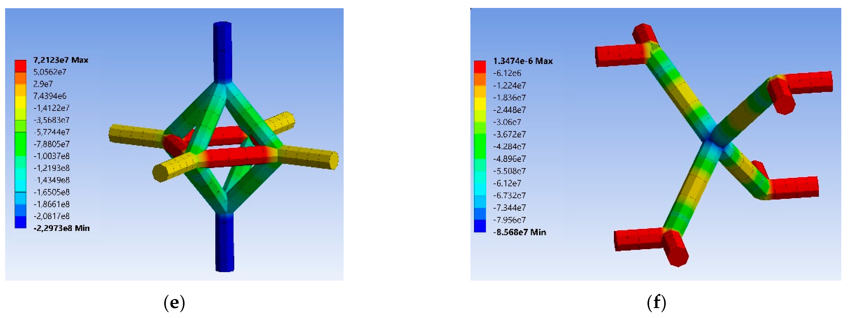
- (a).
- BCC
- (b).
- Diamond
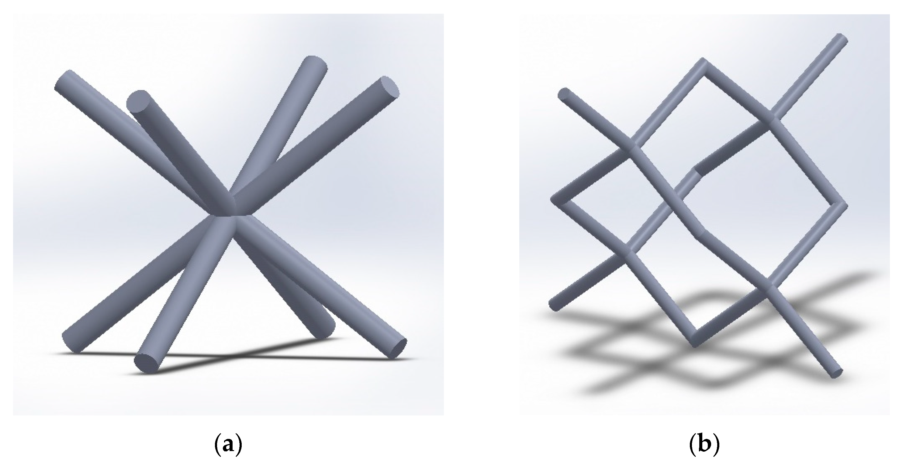
- (c).
- Hexagonal packing
- (d).
- Rhombicuboctahedron
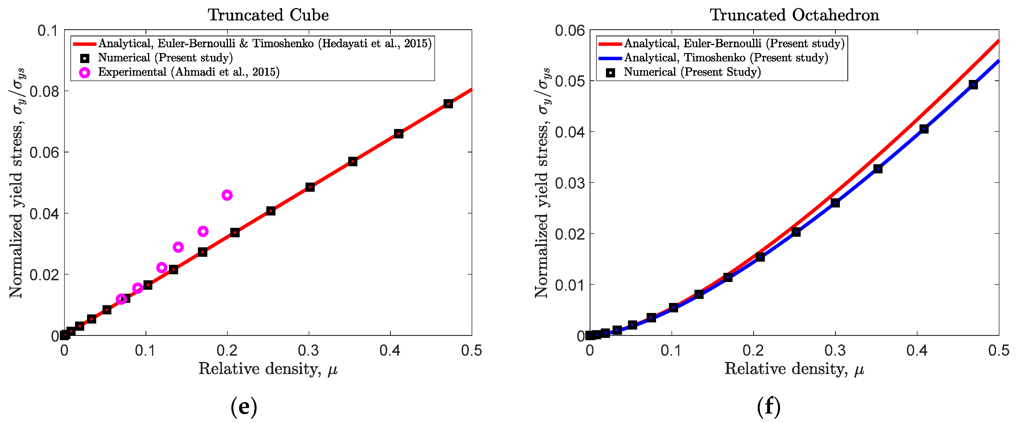
- (e).
- Truncated cube
- (f).
- Truncated octahedron
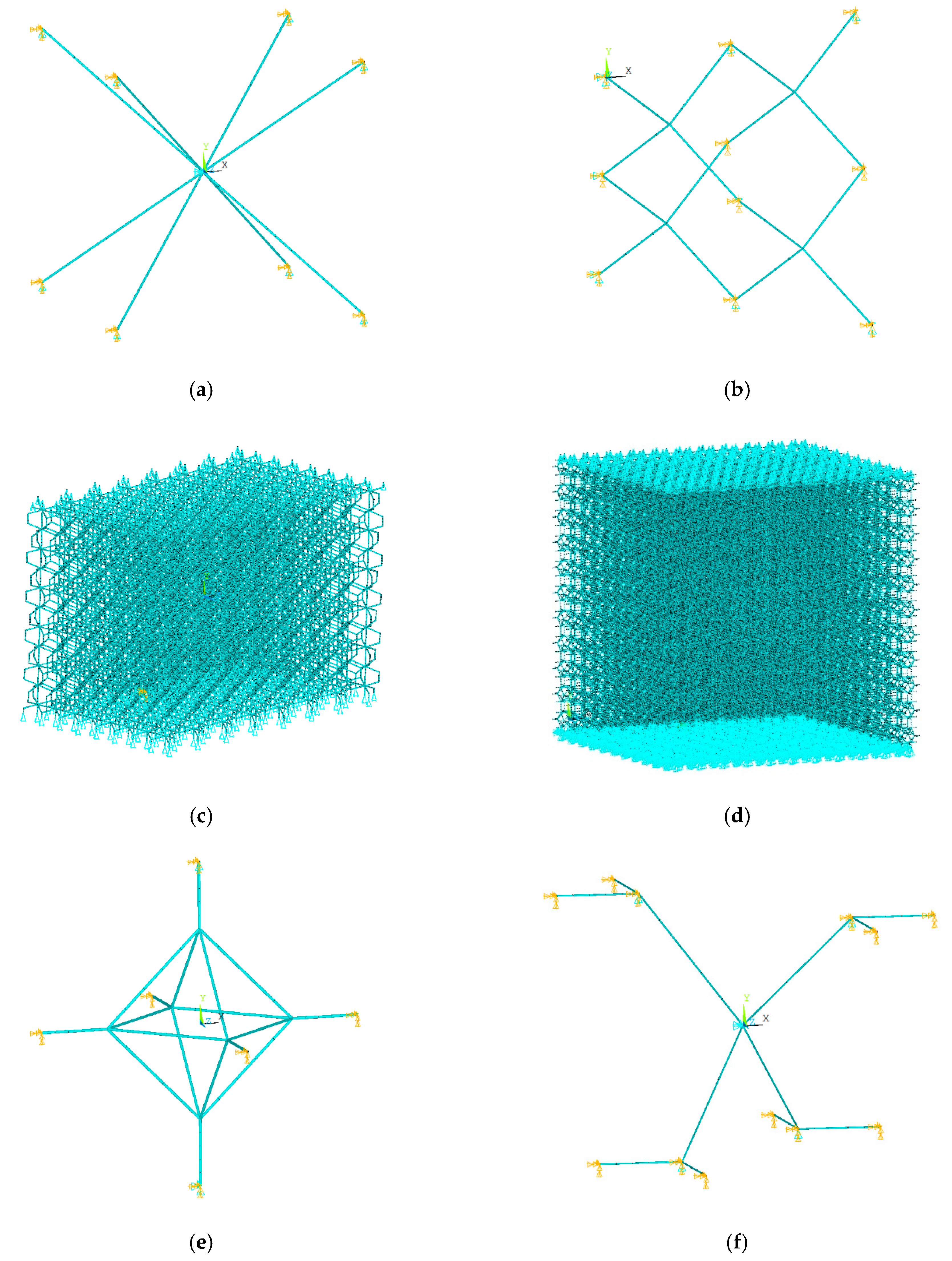
2.4. Numerical Analysis
- Elastic modulus: The formula was used for calculating numerical elastic modulus, where is the structure length in the direction parallel to loading direction, is the cross-sectional area of the structure in the direction perpendicular to the loading direction, is the downward displacement applied to the uppermost nodes, and is obtained by summing the reaction forces of the lowermost nodes.
- Poisson’s ratio: The formula was used for obtaining Poisson’s ratio. In this formula, and are the downward displacement applied to the uppermost nodes and unit cell’s length in the direction parallel to loading direction, respectively. Parameters and are respectively the lateral displacement of the side nodes and the structure length in the direction perpendicular to loading direction.
- Yield stress: The formula was used to calculate normalized yield stress. In this formula, is the maximum von Mises stress experienced in the most critical point of the structure. The critical points of each unit cell can be seen in Section 4.1.
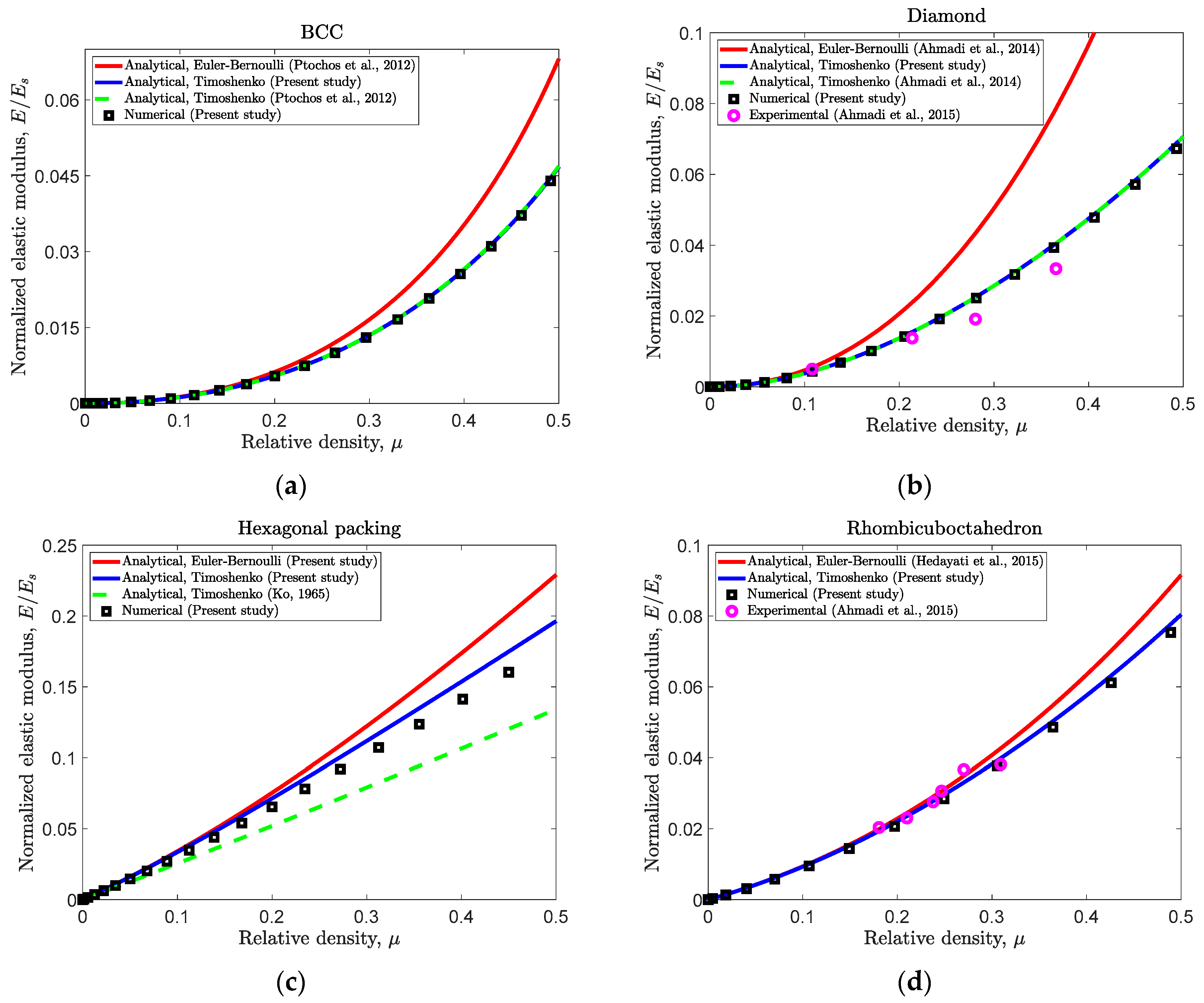
3. Results
4. Discussions
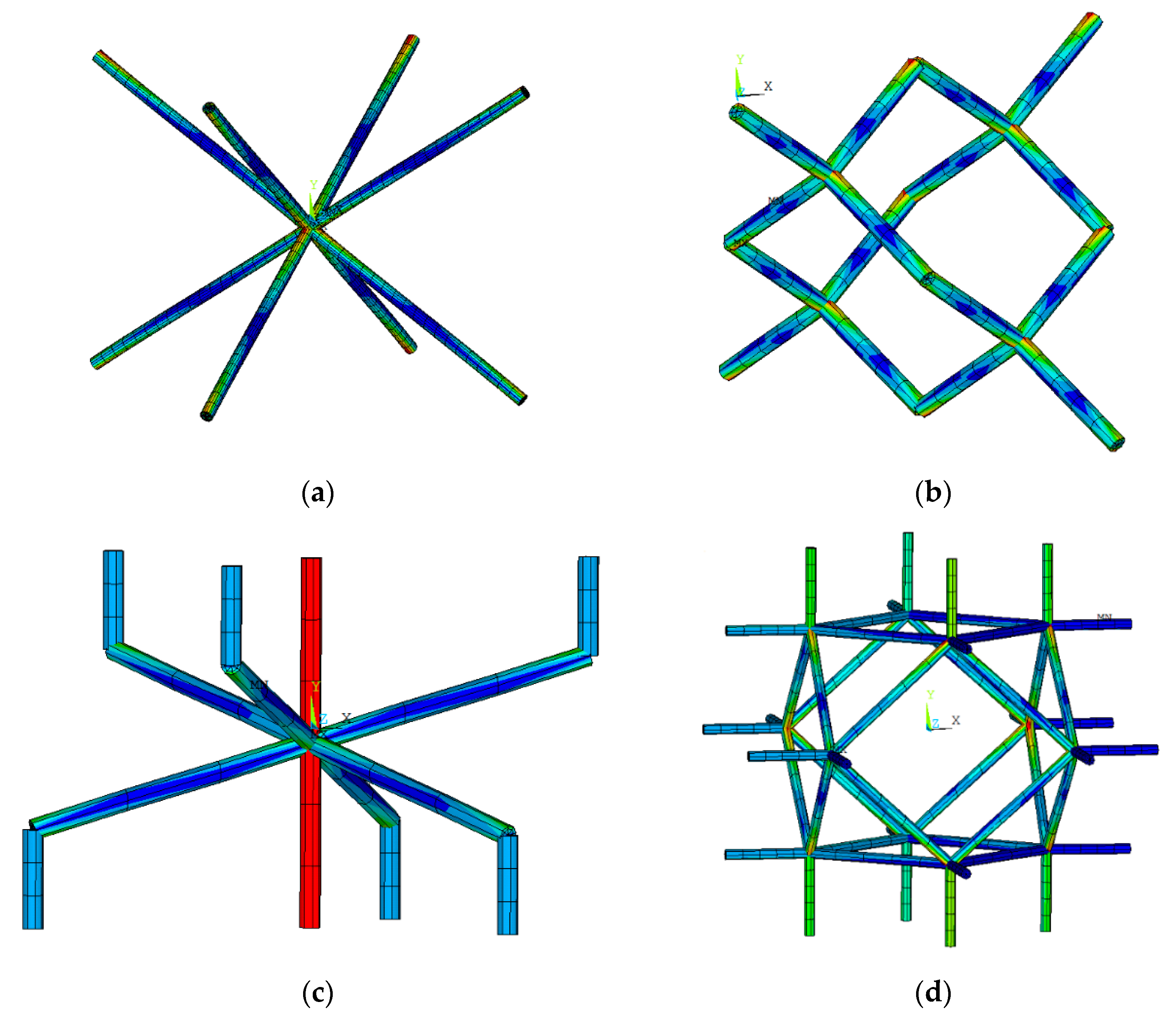
4.1. Unit Cell’s Behaviour
4.2. Why the New Relationships Give Much Better Accuracy?
4.3. Yield Strength
4.4. Some Points Regarding Experimental Data Points
4.5. Application to Biomedical Implants
4.6. Limitations of the Present Approach
5. Conclusions
Author Contributions
Funding
Institutional Review Board Statement
Informed Consent Statement
Data Availability Statement
Conflicts of Interest
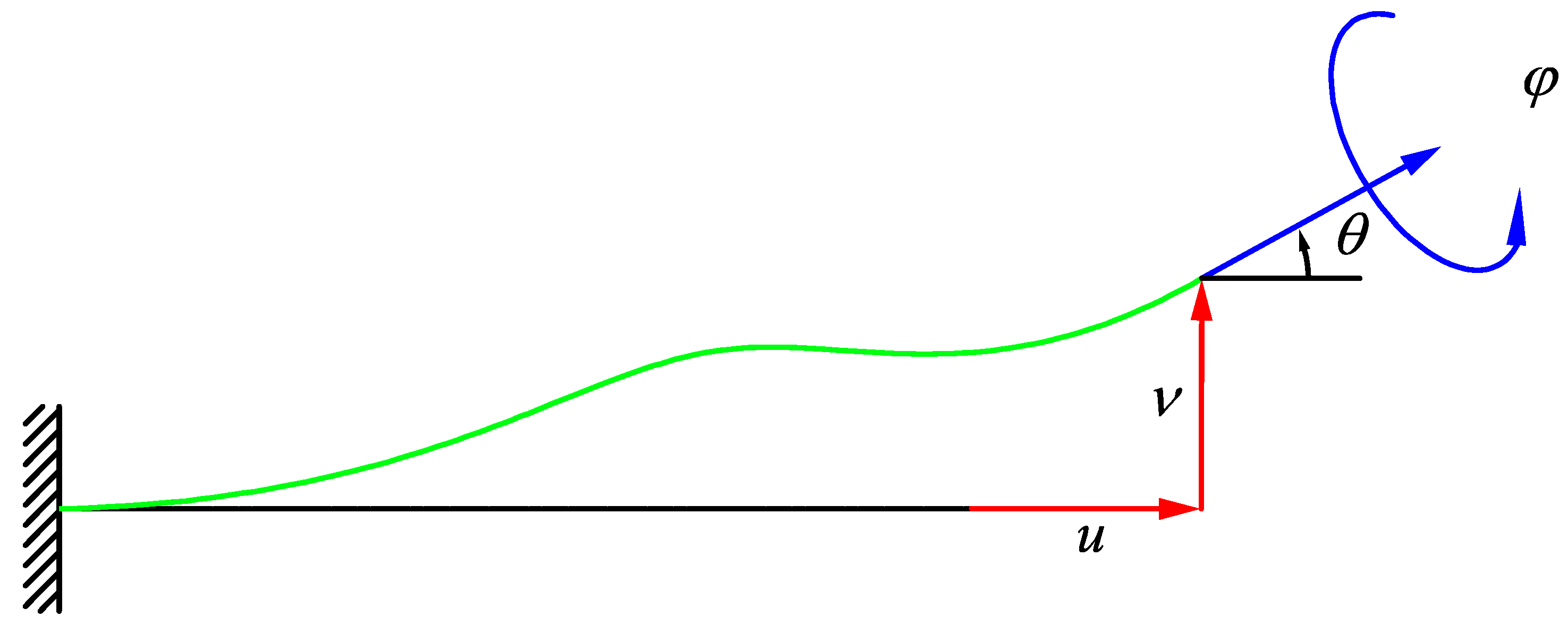
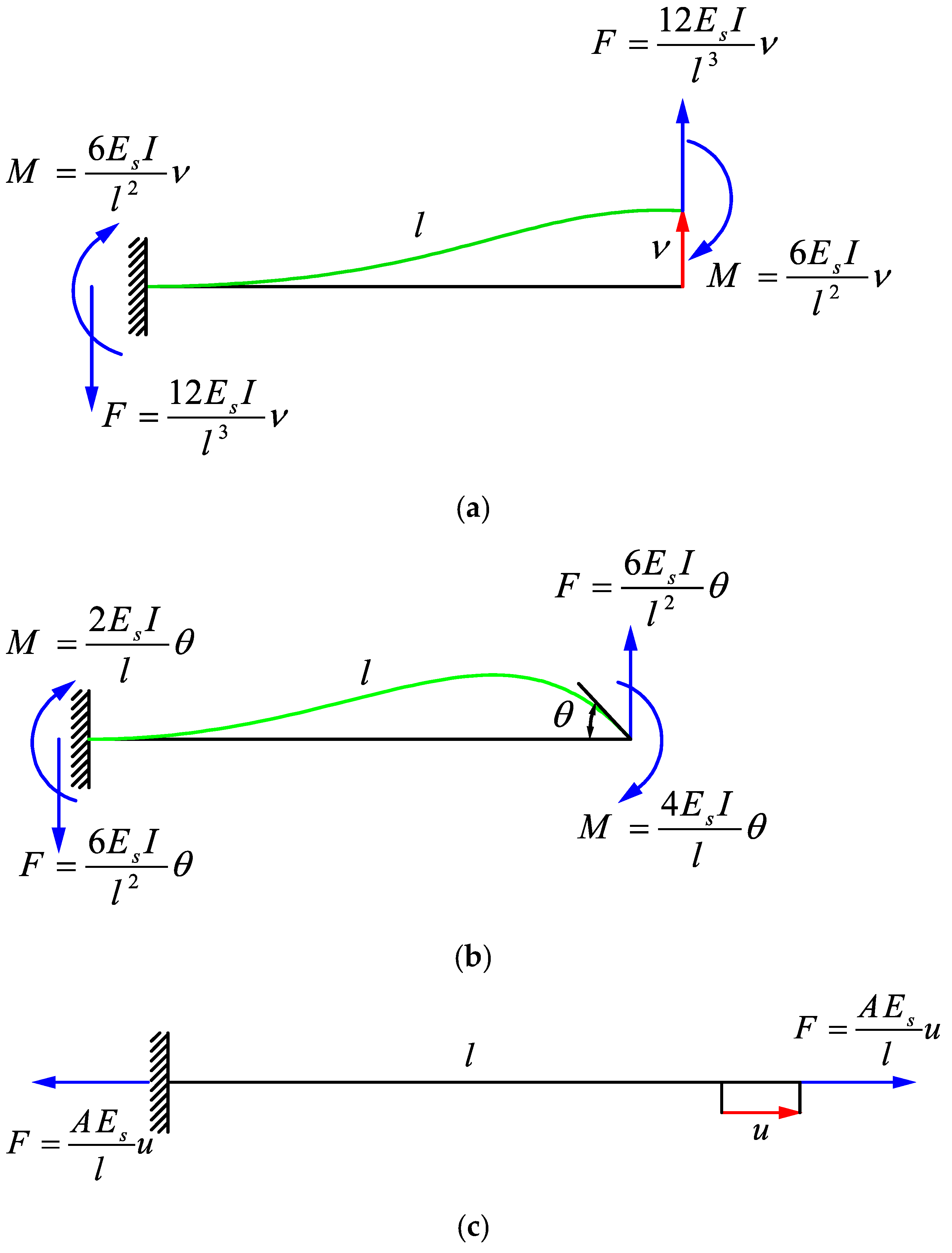
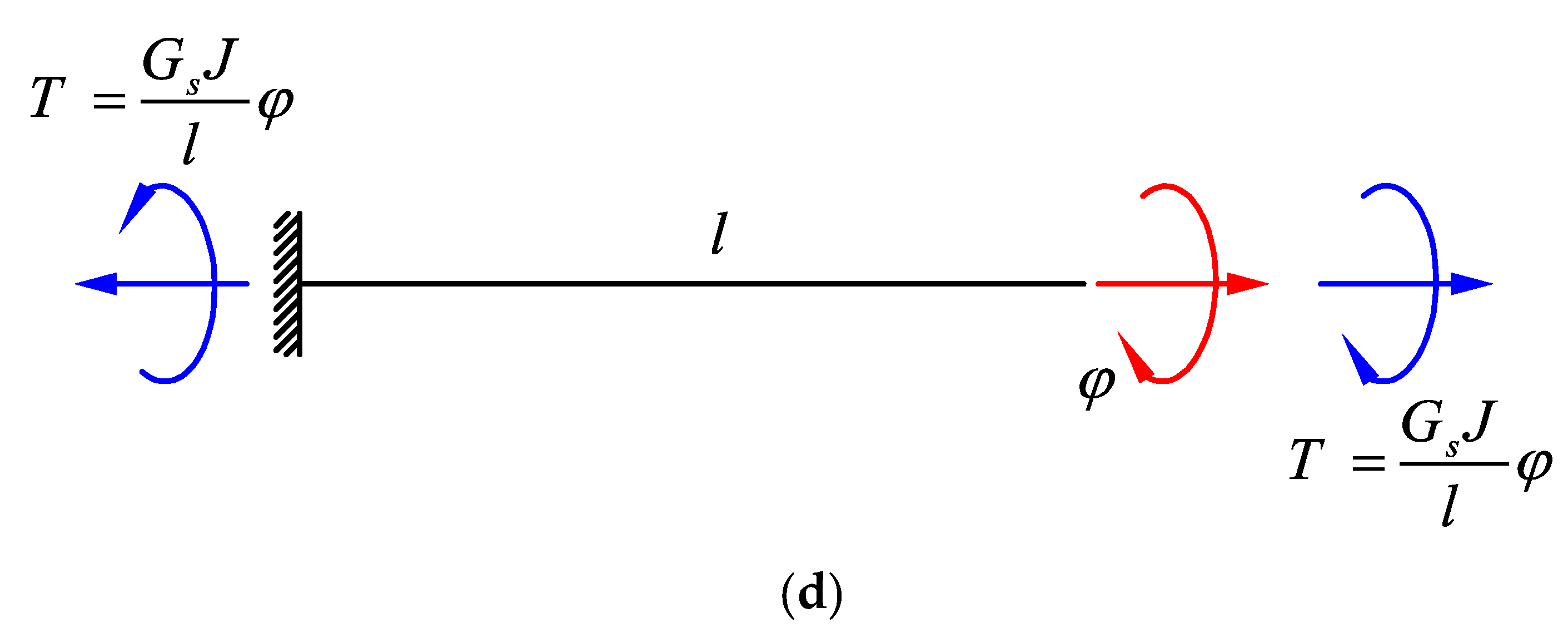
Appendix A. Derivation of Forces and Moments for a Single Strut
Appendix A.1. Cantilever Beam with Displacement without Rotation in the End
- (A)
- (B)
- (C)
- (D)
- (A)
- (B)
Appendix A.2. Cantilever Beam with Rotation without Displacement in the End
- (A)
- (B)
- (C)
- (D)
- (E)
- (F)
Appendix B. Analytical Equations Extracted from the Literature

Appendix C. New Analytical Relationships for Hexagonal Packing Geometry


Appendix D. Stress and Strain Contours in the Lattice Structures


Appendix E. Effect of Considering Shear Deformation on the Forces/Moments of a Single Strut

References
- Pałka, K.; Pokrowiecki, R. Porous Titanium Implants: A Review. Adv. Eng. Mater. 2018, 20, 1700648. [Google Scholar] [CrossRef]
- Hedayati, R.; Sadighi, M. Low-velocity impact behaviour of open-cell foams. J. Theor. Appl. Mech. 2018, 56, 939–949. [Google Scholar] [CrossRef]
- Torres, Y.; Pavón, J.; Rodríguez, J. Processing and characterization of porous titanium for implants by using NaCl as space holder. J. Mater. Process. Technol. 2012, 212, 1061–1069. [Google Scholar] [CrossRef]
- Hedayati, R.; Ahmadi, S.; Lietaert, K.; Tümer, N.; Li, Y.; Yavari, S.A.; Zadpoor, A.A. Fatigue and quasi-static mechanical behavior of bio-degradable porous biomaterials based on magnesium alloys. J. Biomed. Mater. Res. Part A 2018, 106, 1798–1811. [Google Scholar] [CrossRef] [PubMed]
- Gibson, L.J.; Ashby, M.F. Cellular Solids: Structure and Properties; Cambridge University Press: Cambridge, UK, 1999. [Google Scholar]
- Hedayati, R.; Sadighi, M.; Mohammadi-Aghdam, M.; Hosseini-Toudeshky, H. Comparison of elastic properties of open-cell metallic biomaterials with different unit cell types. J. Biomed. Mater. Res. Part B Appl. Biomater. 2018, 106, 386–398. [Google Scholar] [CrossRef] [PubMed]
- Brandl, E.; Heckenberger, U.; Holzinger, V.; Buchbinder, D. Additive manufactured AlSi10Mg samples using Selective Laser Melting (SLM): Microstructure, high cycle fatigue, and fracture behavior. Mater. Des. 2012, 34, 159–169. [Google Scholar] [CrossRef]
- Balla, V.K.; Bodhak, S.; Bose, S.; Bandyopadhyay, A. Porous tantalum structures for bone implants: Fabrication, mechanical and in vitro biological properties. Acta Biomater. 2010, 6, 3349–3359. [Google Scholar] [CrossRef]
- Kerckhofs, G.; Pyka, G.; Moesen, M.; Van Bael, S.; Schrooten, J.; Wevers, M. High-Resolution Microfocus X-Ray Computed Tomography for 3D Surface Roughness Measurements of Additive Manufactured Porous Materials. Adv. Eng. Mater. 2013, 15, 153–158. [Google Scholar] [CrossRef]
- Sumner, D.R.; Galante, J.O. Determinants of stress shielding. Clin. Orthop. Relat. Res. 1991, 274, 202–212. [Google Scholar] [CrossRef]
- Surjadi, J.U.; Gao, L.; Du, H.; Li, X.; Xiong, X.; Fang, N.X.; Lu, Y. Mechanical Metamaterials and Their Engineering Applications. Adv. Eng. Mater. 2019, 21, 1800864. [Google Scholar] [CrossRef]
- Li, G.; Wang, L.; Pan, W.; Yang, F.; Jiang, W.; Wu, X.; Kong, X.; Dai, K.; Hao, Y. In vitro and in vivo study of additive manufactured porous Ti6Al4V scaffolds for repairing bone defects. Sci. Rep. 2016, 6. [Google Scholar] [CrossRef] [PubMed]
- Ahmadi, S.; Hedayati, R.; Li, Y.; Lietaert, K.; Tümer, N.; Fatemi, A.; Rans, C.; Pouran, B.; Weinans, H.; Zadpoor, A. Fatigue performance of additively manufactured meta-biomaterials: The effects of topology and material type. Acta Biomater. 2018, 65, 292–304. [Google Scholar] [CrossRef] [PubMed]
- Hedayati, R.; Ahmadi, S.; Lietaert, K.; Pouran, B.; Li, Y.; Weinans, H.; Rans, C.; Zadpoor, A. Isolated and modulated effects of topology and material type on the mechanical properties of additively manufactured porous biomaterials. J. Mech. Behav. Biomed. Mater. 2018, 79, 254–263. [Google Scholar] [CrossRef] [PubMed]
- Taniguchi, N.; Fujibayashi, S.; Takemoto, M.; Sasaki, K.; Otsuki, B.; Nakamura, T.; Matsushita, T.; Kokubo, T.; Matsuda, S. Effect of pore size on bone ingrowth into porous titanium implants fabricated by additive manufacturing: An in vivo experiment. Mater. Sci. Eng. C 2016, 59, 690–701. [Google Scholar] [CrossRef]
- Epasto, G.; Palomba, G.; D’Andrea, D.; Guglielmino, E.; Di Bella, S.; Traina, F. Ti-6Al-4V ELI microlattice structures manufactured by electron beam melting: Effect of unit cell dimensions and morphology on mechanical behaviour. Mater. Sci. Eng. A 2019, 753, 31–41. [Google Scholar] [CrossRef]
- Xiao, L.; Song, W.; Wang, C.; Liu, H.; Tang, H.; Wang, J. Mechanical behavior of open-cell rhombic dodecahedron Ti–6Al–4V lattice structure. Mater. Sci. Eng. A 2015, 640, 375–384. [Google Scholar] [CrossRef]
- Hedayati, R.; Carpio, A.R.; Luesutthiviboon, S.; Ragni, D.; Avallone, F.; Casalino, D.; Van Der Zwaag, S. Role of Polymeric Coating on Metallic Foams to Control the Aeroacoustic Noise Reduction of Airfoils with Permeable Trailing Edges. Materials 2019, 12, 1087. [Google Scholar] [CrossRef]
- Mohammadi, K.; Movahhedy, M.R.; Shishkovsky, I.; Hedayati, R. Hybrid anisotropic pentamode mechanical metamaterial produced by additive manufacturing technique. Appl. Phys. Lett. 2020, 117, 061901. [Google Scholar] [CrossRef]
- Gonzalez, F.J.Q.; Nuño, N. Finite element modeling of manufacturing irregularities of porous materials. Biomater. Biomech. Bioeng. 2016, 3, 1–14. [Google Scholar] [CrossRef]
- Jahadakbar, A.; Moghaddam, N.S.; Amerinatanzi, A.; Dean, D.; Karaca, H.E.; Elahinia, M. Finite Element Simulation and Additive Manufacturing of Stiffness-Matched NiTi Fixation Hardware for Mandibular Reconstruction Surgery. Bioengineering 2016, 3, 36. [Google Scholar] [CrossRef]
- Mahmoud, D.; Elbestawi, M. Lattice Structures and Functionally Graded Materials Applications in Additive Manufacturing of Orthopedic Implants: A Review. J. Manuf. Mater. Process. 2017, 1, 13. [Google Scholar] [CrossRef]
- Hedayati, R.; Hosseini-Toudeshky, H.; Sadighi, M.; Mohammadi-Aghdam, M.; Zadpoor, A. Multiscale modeling of fatigue crack propagation in additively manufactured porous biomaterials. Int. J. Fatigue 2018, 113, 416–427. [Google Scholar] [CrossRef]
- Badiche, X.; Forest, S.; Guibert, T.; Bienvenu, Y.; Bartout, J.-D.; Ienny, P.; Croset, M.; Bernet, H. Mechanical properties and non-homogeneous deformation of open-cell nickel foams: Application of the mechanics of cellular solids and of porous materials. Mater. Sci. Eng. A 2000, 289, 276–288. [Google Scholar] [CrossRef]
- Geng, X.; Ma, L.; Liu, C.; Zhao, C.; Yue, Z. A FEM study on mechanical behavior of cellular lattice materials based on combined elements. Mater. Sci. Eng. A 2018, 712, 188–198. [Google Scholar] [CrossRef]
- Ahmadi, S.; Campoli, G.; Yavari, S.A.; Sajadi, B.; Wauthlé, R.; Schrooten, J.; Weinans, H.; Zadpoor, A. Mechanical behavior of regular open-cell porous biomaterials made of diamond lattice unit cells. J. Mech. Behav. Biomed. Mater. 2014, 34, 106–115. [Google Scholar] [CrossRef]
- Hedayati, R.; Sadighi, M.; Aghdam, M.; Zadpoor, A. Analytical relationships for the mechanical properties of additively manufactured porous biomaterials based on octahedral unit cells. Appl. Math. Model. 2017, 46, 408–422. [Google Scholar] [CrossRef]
- Babaee, S.; Jahromi, B.H.; Ajdari, A.; Nayeb-Hashemi, H.; Vaziri, A. Mechanical properties of open-cell rhombic dodecahedron cellular structures. Acta Mater. 2012, 60, 2873–2885. [Google Scholar] [CrossRef]
- Ghavidelnia, N.; Hedayati, R.; Sadighi, M.; Mohammadi-Aghdam, M. Development of porous implants with non-uniform mechanical properties distribution based on CT images. Appl. Math. Model. 2020, 83, 801–823. [Google Scholar] [CrossRef]
- Hedayati, R.; Sadighi, M.; Mohammadi-Aghdam, M.; Zadpoor, A. Mechanics of additively manufactured porous biomaterials based on the rhombicuboctahedron unit cell. J. Mech. Behav. Biomed. Mater. 2016, 53, 272–294. [Google Scholar] [CrossRef]
- Ptochos, E.; Labeas, G. Elastic modulus and Poisson’s ratio determination of micro-lattice cellular structures by analytical, numerical and homogenisation methods. J. Sandw. Struct. Mater. 2012, 14, 597–626. [Google Scholar] [CrossRef]
- Hedayati, R.; Sadighi, M.; Mohammadi-Aghdam, M.; Zadpoor, A.A. Mechanical properties of regular porous biomaterials made from truncated cube repeating unit cells: Analytical solutions and computational models. Mater. Sci. Eng. C 2016, 60, 163–183. [Google Scholar] [CrossRef] [PubMed]
- Karaji, Z.G.; Hedayati, R.; Pouran, B.; Apachitei, I.; Zadpoor, A. Effects of plasma electrolytic oxidation process on the mechanical properties of additively manufactured porous biomaterials. Mater. Sci. Eng. C 2017, 76, 406–416. [Google Scholar] [CrossRef] [PubMed]
- Hedayati, R.; Salami, S.J.; Li, Y.; Sadighi, M.; Zadpoor, A. Semianalytical Geometry-Property Relationships for Some Generalized Classes of Pentamodelike Additively Manufactured Mechanical Metamaterials. Phys. Rev. Appl. 2019, 11, 034057. [Google Scholar] [CrossRef]
- Ko, W. Deformations of Foamed Elastomers. J. Cell. Plast. 1965, 1, 45–50. [Google Scholar] [CrossRef]
- Hedayati, R.; Sadighi, M.; Mohammadi-Aghdam, M.; Zadpoor, A. Mechanical behavior of additively manufactured porous biomaterials made from truncated cuboctahedron unit cells. Int. J. Mech. Sci. 2016, 106, 19–38. [Google Scholar] [CrossRef]
- Dementjev, A.; Tarakanov, O. Influence of the cellular structure of foams on their mechanical properties. Mech. Polym. 1970, 4, 594–602. [Google Scholar]
- Cowper, G.R. The Shear Coefficient in Timoshenko’s Beam Theory. J. Appl. Mech. 1966, 33, 335–340. [Google Scholar] [CrossRef]
- Zhu, H.; Knott, J.; Mills, N. Analysis of the elastic properties of open-cell foams with tetrakaidecahedral cells. J. Mech. Phys. Solids 1997, 45, 319–343. [Google Scholar] [CrossRef]
- Ghavidelnia, N.; Bodaghi, M.; Hedayati, R. Analytical relationships for yield stress of five different unit cells. Mech. Based Des. Struct. Mach. 2020, 1–23. [Google Scholar] [CrossRef]
- Ahmadi, S.M.; Yavari, S.A.; Wauthle, R.; Pouran, B.; Schrooten, J.; Weinans, H.; Zadpoor, A.A. Additively Manufactured Open-Cell Porous Biomaterials Made from Six Different Space-Filling Unit Cells: The Mechanical and Morphological Properties. Materials 2015, 8, 1871–1896. [Google Scholar] [CrossRef]


| Term | Euler–Bernoulli Theory | Timoshenko Theory |
|---|---|---|
| Axial Tension/Compression | ||
| Torsion | ||
| Lateral deformation Force | ||
| Lateral deformation Moment | ||
| Rotation Force | ||
| Rotation Moment |
| Unit Cell | ||
|---|---|---|
| Euler–Bernoulli Theory | Timoshenko Theory | |
| BCC | [31] | |
| Diamond | [26] | |
| Hexagonal packing | (see Appendix C) | |
| Rhombicuboctahedron | [30] | |
| Truncated cube | [32] | |
| Truncated octahedron | [39] | |
| Unit Cell | Poisson’s Ratio, | |
| Euler–Bernoulli Theory | Timoshenko Theory | |
| BCC | [31] | |
| Diamond | [26] | |
| Hexagonal packing | (see Appendix C) | |
| Rhombicuboctahedron | [30] | |
| Truncated cube | [32] | |
| Truncated octahedron | [39] | |
| Unit Cell | ||
|---|---|---|
| Euler–Bernoulli Theory | Timoshenko Theory | |
| BCC | [40] | |
| Diamond | [40] | |
| Hexagonal packing | [40] | |
| Rhombicuboctahedron | * (See the footnote of the table) | |
| Truncated cube | [4] | |
| Truncated octahedron | [40] | |
Publisher’s Note: MDPI stays neutral with regard to jurisdictional claims in published maps and institutional affiliations. |
© 2021 by the authors. Licensee MDPI, Basel, Switzerland. This article is an open access article distributed under the terms and conditions of the Creative Commons Attribution (CC BY) license (http://creativecommons.org/licenses/by/4.0/).
Share and Cite
Hedayati, R.; Ghavidelnia, N.; Sadighi, M.; Bodaghi, M. Improving the Accuracy of Analytical Relationships for Mechanical Properties of Permeable Metamaterials. Appl. Sci. 2021, 11, 1332. https://doi.org/10.3390/app11031332
Hedayati R, Ghavidelnia N, Sadighi M, Bodaghi M. Improving the Accuracy of Analytical Relationships for Mechanical Properties of Permeable Metamaterials. Applied Sciences. 2021; 11(3):1332. https://doi.org/10.3390/app11031332
Chicago/Turabian StyleHedayati, Reza, Naeim Ghavidelnia, Mojtaba Sadighi, and Mahdi Bodaghi. 2021. "Improving the Accuracy of Analytical Relationships for Mechanical Properties of Permeable Metamaterials" Applied Sciences 11, no. 3: 1332. https://doi.org/10.3390/app11031332
APA StyleHedayati, R., Ghavidelnia, N., Sadighi, M., & Bodaghi, M. (2021). Improving the Accuracy of Analytical Relationships for Mechanical Properties of Permeable Metamaterials. Applied Sciences, 11(3), 1332. https://doi.org/10.3390/app11031332