Cocrystal Prediction Using Machine Learning Models and Descriptors

Abstract

Cocrystals are of much interest in industrial application as well as academic research, and screening of suitable coformers for active pharmaceutical ingredients is the most crucial and challenging step in cocrystal development. Recently, machine learning techniques are attracting researchers in many fields including pharmaceutical research such as quantitative structure-activity/property relationship. In this paper, we develop machine learning models to predict cocrystal formation. We extract descriptor values from simplified molecular-input line-entry system (SMILES) of compounds and compare the machine learning models by experiments with our collected data of 1476 instances. As a result, we found that artificial neural network shows great potential as it has the best accuracy, sensitivity, and F1 score. We also found that the model achieved comparable performance with about half of the descriptors chosen by feature selection algorithms. We believe that this will contribute to faster and more accurate cocrystal development.

1. Introduction

Active pharmaceutical ingredients (APIs) are commonly formulated and delivered to patients in the solid dosage forms (tablets, capsules, powders) for reasons of economy, stability, and convenience of intake [1]. One of the major problems faced during the formulation of drug is its low bioavailability which is mainly reliant on the solubility and permeability of API [2,3], and one of the approaches to enhance the physicochemical and pharmacological properties of API without modifying its intrinsic chemical structure is to develop novel solid forms such as cocrystals [4,5,6,7]. There are extensive reports on cocrystals for the purpose of improving the pharmaceutical properties including dissolution, permeability, bioavailability, stability, photostability, hygroscopicity, and compressibility [8,9].

Cocrystals are much of interest in industrial application as well as academic research because they offer various opportunities for intellectual property rights in respect of the development of new solid forms [10]. Furthermore, the latest Food and Drug Administration (FDA) guidance on pharmaceutical cocrystals, which recognizes cocrystals as drug substances, provides an excellent opportunity for the pharmaceutical industry to develop commercial products of cocrystals [11,12]. According to FDA, cocrystals are “Crystalline materials composed of two or more molecules within the same crystal lattice” [13]. Pharmaceutical cocrystals, a subclass of cocrystals, are stoichiometric molecular complexes composed of APIs and pharmaceutically acceptable coformers held together by non-covalent interactions such as hydrogen bonding within the same crystal lattice [14]. Coformers for pharmaceutical cocrystallization should be from the FDA’s list of Everything Added to Food in the United States (EAFUS) or from the Generally Recognized as Safe list (GRAS), as they should have no adverse or pharmacological toxic effects [1]. The list of acceptable co-formers, in principle, is likely to at least extend into the hundreds, which means that screening of suitable coformers for an API is the most crucial and challenging step in cocrystal development [15]. Since experimental determination of cocrystals is time-consuming, costly, and labor-intensive, it is valuable to develop complementary tools that can reduce the list of coformers by predicting which coformers are likely to form cocrystals [16].

Various knowledge-based and computational approaches have been used in the literature to predict cocrystal formation. Supramolecular synthesis introduced by Desiraju is a well-known approach to rationalize the possibility of cocrystal formation [17,18,19]. A common strategy in this method is to first identify the crystal structure of the target molecule and investigate coformers with a desired functional group which can form intermolecular interactions (mainly hydrogen bonding) between the target molecule and coformers [15]. Knowledge of synthons allows the selection of potential coformers and predicts the interaction outcomes, but there is no guarantee that cocrystals with predicted structures would form. Statistical analysis of cocrystal data from the Cambridge Structural Database (CSD) where more than one million crystal structures of small molecules are available, allows researchers to apply virtual screening techniques to find suitable cocrystal-forming pairs [20]. Galek et al. introduced hydrogen-bond propensity as a predictive tool and determined the likelihood of co-crystal formation [15,21]. Fábián analyzed the possibility of cocrystal formation by correlating the different descriptors such as polarity and molecular shape [22]. Cocrystal design can also be based on computational approaches, including the use of the $\Delta$pK value [23,24], lattice energy calculation [25,26,27,28], molecular electrostatic potential surfaces (MEPS) calculation [29,30,31,32], Hansen solubility parameters calculation [33,34] and Conductor like screening Model for Real solvents (COSMO-RS) based enthalpy of mixing calculation [35,36,37,38].

In recent years, machine-learning (ML) has emerged as promising tool for data-driven predictions in pharmaceutical research, such as quantitative structure-activity/property relationships (QSAR/QSPR), drug-drug interactions, drug repurposing and pharmacogenomics [39]. In the area of pharmaceutical cocrystal research, Rama Krishna et al. applied artificial neural network to predict three solid-state properties of cocrystals, including melting temperature, lattice energy, and crystal density [40]. Przybylek et al. developed cocrystal screening models based on simple classification regression and Multivariate Adaptive Regression Splines (MARSplines) algorithm using molecular descriptors for phenolic acid coformers and dicarboxylic acid coformers, respectively [41]. Wicker et al. created a predictive model, that can classify a pair of coformers as a possible cocrystal or not, using a support vector machine (SVM) and simple descriptors of coformer molecules to guide the selection of coformers in the discovery of new cocrystals [16]. Devogelaer and co-workers introduced a comprehensive approach to study cocrystallization using network science and linkage prediction algorithms and constructed a data-driven co-crystal prediction tool with co-crystal data extracted from the CSD [42]. Wang et al. also used a data set with co-crystal data available in the CSD and ultimately developed a machine learning model using different model types and molecular fingerprints that can be used to select appropriate coformers for a target molecule [43]. The above existing studies have shown successful results, but they have a common limitation that they only compared model performance (e.g., accuracy) without investigating features (i.e., descriptors) importance.

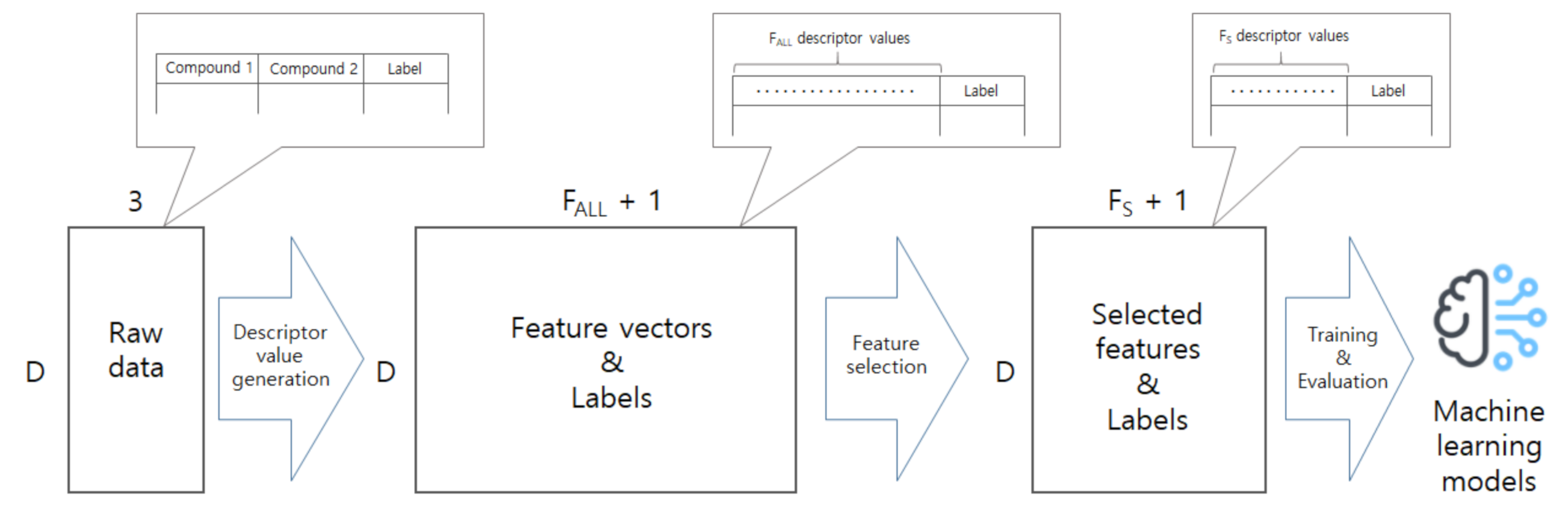
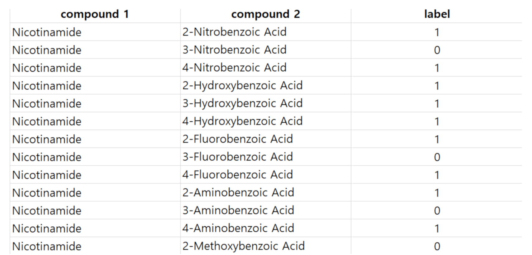
In this work, we develop a model to predict co-crystal formation of API molecules. We use Mordred [44], one of widely-used descriptor calculators, to extract descriptor values from simplified molecular-input line-entry system (SMILES) strings of API and coformers compounds. There are several other tools or molecular descriptor-calculators used in cheminformatics such as PaDEL [45], PyDPI [46], Rcpi [47], Dragon [48], BlueDesc (http://www.ra.cs.uni-tuebingen.de/software/bluedesc) and cinfony [49]; PaDEL descriptor-calculator is the most well-known tool and provides 1875 descriptors, and cinfony is a collection or a wrapper of other libraries such as Open Babel [50], RDKit (http://www.rdkit.org), and Chemistry Development Kit (CDK) [51]. We chose to use Mordred and used the descriptor values as features and compared different machine learning models through experimental results using our collected data. Our contributions can be summarized as follows. First, we not only extract descriptor values of compound pairs, but also investigate which descriptors are more important, and show that we can achieve good performance even if we use only a small subset of the descriptors. Second, we compare machine learning models through experiments and find that artificial neural networks (ANN) achieve the best performance. Third, we make our dataset available for free through the online website (http://ant.sch.ac.kr/) so that many other researchers can use the dataset as a benchmark. We believe that this study will advance the field of cocrystal formation prediction, and our dataset will help other researchers to easily develop better models.

2. Materials and Methods

In this paper, we essentially solve a binary classification problem; we develop a model for predicting a label (e.g., ‘fail’ and ‘success’) for a given pair of compounds. The class label ‘success’ means that the corresponding pair of compounds would successfully cocrystallize, while the label ‘fail’ means that it would not cocrystallize. As depicted in Figure 1, we first obtain attributes (i.e., features) of the compounds. Then, we select some promising features that are expected to contribute more to the final performance (e.g., accuracy). The selected features are fed into machine learning models that learn patterns behind the compound pairs, so that the models predict labels (e.g., ‘success’, ‘fail’) of the given pairs; in other words, the model takes the selected features obtained from compound pairs as input and generates labels as output.

2.1. Materials

Since we basically solve this problem using a data-driven approach, we first had to prepare a data set. The compounds pairs of the data set were mainly obtained from the work of Wicker et al. [16], Przybylek et al. [41,52] and Grecu et al. [32] and supplemented with an extensive literature review on cocrystal screening of different APIs. Duplicate records were removed from the data set, resulting in a total of 1476 molecular compound pairs. Of these 1476 pairs, 753 were positive pairs (experimentally verified cocrystals) and the remaining 723 were negative pairs (unsuccessful formation of cocrystals). Labels are converted to a numerical form (e.g., ‘success’ = 1, and ‘fail’ = 0). The raw data is a $D\times 3$ matrix and samples are shown in Figure 2. We primarily develop models that predict which pair of API (i.e., ‘compound 1’) and coformer (i.e., ‘compound 2’) will successfully result into a new cocrystal formation (i.e., ‘label’ = 1) and which will not result in a new solid form (i.e., ‘label’ = 0), from the set of chemical experiments based on the two columns (e.g., ‘compound 1’ and ‘compound 2’) as shown in Figure 2. Prediction models use a combination of features known as molecular descriptors from each pair for the classification task.

Molecular descriptors often used to develop quantitative structure-property relationships (QSPR) models, and Mordred is one of the attractive tools to extract the molecular descriptors [44]. We have chosen Mordred because of its advantages: (1) it provides a comparable number of PaDEL descriptors while fixing some bugs within the PaDEL descriptor calculator, and (2) it is easy to install and use since it is provided as Python 2 & 3 libraries. As shown on the left in Figure 1, the Mordred tool used to extract feature vectors from the raw data. Canonical SMILES strings for each compound were retrieved from PubChem (https://pubchem.ncbi.nlm.nih.gov/) as shown in

Table 1. Sample of canonical SMILES strings by PubChem for each compound in a sample of raw data.

Service	Compound 1	Compound 2	Label
PubChem	C1=CC(=CN=C1)C(=O)N	C1=CC=C(C(=C1)C(=O)O)[N+](=O)[O-]	1
	C1=CC(=CN=C1)C(=O)N	C1=CC(=CC(=C1)[N+](=O)[O-])C(=O)O	0
	C1=CC(=CN=C1)C(=O)N	C1=CC(=CC=C1C(=O)O)[N+](=O)[O-]	1
	C1=CC(=CN=C1)C(=O)N	C1=CC=C(C(=C1)C(=O)O)O	1
	C1=CC(=CN=C1)C(=O)N	C1=CC(=CC(=C1)O)C(=O)O	1
	C1=CC(=CN=C1)C(=O)N	C1=CC(=CC=C1C(=O)O)O	1
	C1=CC(=CN=C1)C(=O)N	C1=CC=C(C(=C1)C(=O)O)F	1
	C1=CC(=CN=C1)C(=O)N	C1=CC(=CC(=C1)F)C(=O)O	0
	C1=CC(=CN=C1)C(=O)N	C1=CC(=CC=C1C(=O)O)F	1
	C1=CC(=CN=C1)C(=O)N	C1=CC=C(C(=C1)C(=O)O)N	1
	C1=CC(=CN=C1)C(=O)N	C1=CC(=CC(=C1)N)C(=O)O	0
	C1=CC(=CN=C1)C(=O)N	C1=CC(=CC=C1C(=O)O)N	1
	C1=CC(=CN=C1)C(=O)N	COC1=CC=CC=C1C(=O)O	0

, and were used as input to the Mordred tool to generate molecular descriptor values. We found that some descriptor values are missing due to implementation issues of the tool; for example, a part of autocorrelation descriptor of a small molecule is known to be missing even if there is no bug [44]. Since the missing values did not occur at random, we simply filter them out instead of using any imputation algorithms. We obtain a $F_{ALL}$ dimensional real-numbered feature vector from a single pair of compounds. After adding a label column, we have D feature vectors of $F_{ALL}+1$ dimension.

2.2. Methods

There have been studies that trained machine learning models using molecular descriptors as features [16,53], however such studies only fed the models with the descriptors without performing a crucial analysis of the molecular descriptors. In this work, we apply feature selection algorithms to measure importance of descriptors and use a found set of promising ones. The feature selection algorithms are supposed to select $F_S$ features among the $F_{ALL}$ features as depicted in the middle of Figure 1. We tried two feature selection algorithms: Recursive Feature Elimination (RFE) algorithm and K-best algorithm. The RFE algorithm is a wrapper-based algorithm that treats the feature selection as a search problem. It repeatedly removes unpromising features until desired number of features remains. We use an artificial neural network (ANN) as an estimator of the RFE algorithm. The K-best algorithm is a filter-based algorithm that selects potential features according to a particular function $\sigma (f,c)$ where f and c are a feature and a label, respectively. We use a ANOVA F-value as the function $\sigma$.

Before passing the $D\times F_S+1$ real-numbered matrix to machine learning models, we standardize the feature values. This process is, of course, performed using only training data; the mean $\mu$ and standard deviation $\sigma$ are computed only with the training data. We used scikit-learn (https://scikit-learn.org/stable/) to implement the standardization, and found that it is better than normalization (i.e., 0–1 scaling) for our data. Given the standardized matrix $\mathbf{X}\in {\mathbb{R}}^{D\times F_S}$, the machine learning models are supposed to give labels $\mathbf{y}\in {\{0,1\}}^D$. We have used several machine learning models such as artificial neural network (ANN), support vector machine (SVM) [54], random forest (RF) [55], and extreme gradient boost (XGB) [56]. The ANN is known to be effective in many research fields such as image analysis, natural language processing, and speech recognition; It is a deep learning model if it has a deep structure (i.e., multiple hidden layers). The SVM finds a decision boundary based on boundary instances (i.e., support vectors) and is known to be successful in many classification tasks. The RF and XGB are common ensemble approaches, but RF uses the bagging strategy while the XGB employs boosting strategy. We compared these widely-used models with experimental results.

The total, the dataset $D_{total}$ contains 1476 instances, of which 723 were unsuccessful, and 753 were successful, as shown in

Table 2. Data statistics.

	All Labels	Label ‘Success’	Label ‘Fail’
# of data	1476	753	723

. Since the dataset is balanced, we performed 10-fold cross validation while maintaining the balanced ratio; for each cross validation, we have about 1,329 instances for training and 147 instances for testing. After preprocessing the raw data, we obtained that $F_{ALL}$ = 2207. Throughout all experimental results, we use averaged accuracy, precision, recall, and F1 scores.

3. Results

3.1. Feature Selection Algorithms

We compared the two feature selection algorithms (e.g., RFE algorithm and K-best algorithm) by averaged accuracy with varying number of features $F_S$. Figure 3 shows the results with $F_S$ ranging from 298 to 1103, where the classifier used here is artificial neural network (ANN); note that we use only ANN model because we focus on experimental results of feature selection algorithms, but not the models. With greater $F_S$, the K-best algorithm gave generally better accuracies than the RFE algorithm. Therefore, we might say that if we want efficiency (e.g., less parameters), then the RFE algorithm will be preferable; on the other hand, the K-best algorithm is preferable if we want effectiveness (e.g., accuracy). As a compromise, using the K-best algorithm with $F_S=900$ might be a reasonable choice because its dimension is only a half of the total (e.g., 2207) and its accuracy is comparable.

3.2. Model Comparison

We prepared three independent datasets $D_{total}^1$, $D_{total}^2$, and $D_{total}^3$ by shuffling the instances of the dataset $D_{total}$; so $|D_{total}|$ = $|D_{total}^1|$ = $|D_{total}^2|$ = $|D_{total}^3|$ = 1476. We conducted 10-fold cross validation for each of these independent datasets, and computed averaged accuracy, precision, recall, and F1 scores. The optimal parameter settings of the machine learning models are found by a grid searching using a small portion (e.g., 10%) of the training set as a validation set. The parameter settings are summarized in

Table 3. Parameter settings of machine learning models.

Model	Setting
Random forest	Number of estimators = 100
(RF)	No limitation of depth
	Minimum samples for splitting = 2
Support vector machine	Kernel = Linear
(SVM)	C = 1.0
Extreme gradient boosting	Number of estimators = 100
(XGB)	Learning rate = 0.3
	# of hidden layers = 2
Artificial neural network	Hidden layer sizes (# of nodes of each layer) = 25
(ANN)	Activation function = Relu function [57]
	Optimizer = Adam [58]
	# of epochs = 50 with early stopping

; the parameter settings are obtained during the experiments. The ANN has a shallow structure (i.e., one hidden layer of 25 nodes) because we found that it gives better performance than other complex structure; the reason might be the small size of dataset that high model complexity will cause overfitting problem.

Table 4. Averaged accuracy of different machine learning models, where $F_{ALL}$ is the number of all features, and $F_S$ means the number of features selected using the K-best algorithm.

Model	All Features (${\mathit{F}}_{\mathit{ALL}}$ = 2207)	${\mathit{F}}_{\mathit{S}}$ = 1103	${\mathit{F}}_{\mathit{S}}$ = 900
RF	0.829	0.822	0.823
SVM	0.746	0.757	0.758
XGB	0.832	0.823	0.826
ANN	0.833	0.829	0.823

summarizes the accuracy of machine learning models; note that we focus on the experimental comparison between the models here, but not the feature selection algorithms. The accuracy values are computed by averaging results with three independent datasets (e.g., $D_{total}^1$, $D_{total}^2$, and $D_{total}^3$). The ANN gives the best accuracy (e.g., 0.833) among the models. The XGB is comparable to the ANN, and it is the best when $F_S$ = 300. As a model works faster when the feature dimension is small, the XGB might be preferable if we want better efficiency (i.e., fast prediction) without losing much accuracy.

One might argue that the model is not useful if its sensitivity is not high enough.

Table 5. Per-label averaged precision of different machine learning models, where $F_{ALL}$ is the number of all features, $F_S$ means the number of features selected using the K-best algorithm, and ‘Success’ and ‘Fail’ mean label 1 and 0, respectively.

Model	All Features (${\mathit{F}}_{\mathit{ALL}}$ = 2207)		${\mathit{F}}_{\mathit{S}}$ = 1103		${\mathit{F}}_{\mathit{S}}$ = 900
	Fail	Success	Fail	Success	Fail	Success
RF	0.781	0.834	0.839	0.888	0.810	0.854
SVM	0.699	0.781	0.789	0.789	0.740	0.786
XGB	0.782	0.841	0.865	0.890	0.816	0.859
ANN	0.802	0.838	0.803	0.819	0.804	0.831

and

Table 6. Per-label averaged recall of different machine learning models, where $F_{ALL}$ is the number of all features, $F_S$ means the number of features selected using the K-best algorithm, and ‘Success’ and ‘Fail’ mean label 1 and 0, respectively.

Model	All Features (${\mathit{F}}_{\mathit{ALL}}$ = 2207)		${\mathit{F}}_{\mathit{S}}$ = 1103		${\mathit{F}}_{\mathit{S}}$ = 900
	Fail	Success	Fail	Success	Fail	Success
RF	0.840	0.773	0.890	0.836	0.856	0.807
SVM	0.806	0.667	0.778	0.800	0.792	0.733
XGB	0.847	0.773	0.889	0.867	0.861	0.813
ANN	0.835	0.800	0.808	0.808	0.827	0.806

are per-label precision and recall. The ANN gives the best recall of ‘success’ label (e.g., 0.800) without losing much precision (e.g., 0.838). In terms of the precision, the XGB seems the best as its precision of ‘success’ label is 0.841, but we might say that the ANN would be chosen if we need to find as many promising candidates of compound pairs as possible.

Table 7. Per-label averaged F1 score of different machine learning models, where $F_{ALL}$ is the number of all features, $F_S$ means the number of features selected using the K-best algorithm, and ‘Success’ and ‘Fail’ mean label 1 and 0, respectively.

Model	All Features (${\mathit{F}}_{\mathit{ALL}}$ = 2207)		${\mathit{F}}_{\mathit{S}}$ = 1103		${\mathit{F}}_{\mathit{S}}$ = 900
	Fail	Success	Fail	Success	Fail	Success
RF	0.809	0.803	0.864	0.861	0.832	0.830
SVM	0.748	0.719	0.783	0.795	0.765	0.759
XGB	0.813	0.806	0.877	0.878	0.838	0.836
ANN	0.817	0.817	0.804	0.812	0.814	0.817

shows per-label F1 scores, and the ANN is turned out to be the best amongst the models. This result is reasonable as the ANN is known to be effective in finding underlying patterns and gives significant performance improvement in many other classification tasks (e.g., malware detection [59], chatbot intent prediction [60]). We believe that the performance will be further improved if we collect more qualified data.

4. Discussion

Although the models performed best when we use all features, the feature selection algorithms showed their potential using only half of the features (e.g., $F_S=1103$ or 900) gave comparable results. One might want to see what features were valuable than others.

Table 8. Best & worst features selected by K-best algorithm with $F_S$ = 900.

30 Best Features			30 Worst Features
Module	Name	Score	Module	Name	Score
	GATS3c	79.718	Aromatic	nAromAtom	0.136
	GATS6c	85.965		AATS7m	0.628
	GATS8c	136.802		ATSC7p	0.007
	GATS6dv	161.104		AATSC8s	0.016
	GATS4s	172.971		AATSC5are	0.017
Autocorrelation	GATS6s	175.205		MATS7dv	0.521
	GATS3Z	80.696		MATS5s	0.027
	GATS6Z	81.969		MATS7s	0.039
	GATS7Z	84.171		MATS8Z	0.195
	GATS8Z	84.774		MATS3v	0.357
	ATS2m	86.768	Autocorrelation	MATS3se	0.001
	MATS5are	90.363		MATS5pe	0.390
	SpDiam_A	85.488		MATS6p	0.477
AdjacencyMatrix	VE3_A	78.929		GATS1c	0.322
	VE1_A	77.862		GATS6d	0.117
Chi	AXp-7dv	82.701		GATS3s	0.469
	SZ	79.156		GATS1i	0.004
Constitutional	Mare	82.745		GATS5i	0.264
	Mp	79.163		GATS7i	0.166
DetourMatrix	DetourIndex	80.610		GATS8i	0.004
	NsssP	81.691		BCUTd-1h	0.474
	NdsssP	78.913		BCUTd-1l	0.361
	NsBr	81.782	BCUT	BCUTv-1l	0.584
	SssNH	81.836		BCUTpe-1h	0.019
EState	SaaNH	79.010		BCUTi-1l	0.004
	SssssGe	82.422	BaryszMatrix	SpAD_DzZ	0.213
	SsAsH2	79.068		SIC3	0.201
	MINssPH	91.111	InformationContent	CIC0	0.169
	NssSnH2	78.956		MIC3	0.240
ExtendedTopochemicalAtom	ETA_epsilon_5	78.193	MoRSE	Mor06p	0.303

shows lists of best and worst features obtained by K-best algorithm with $F_S$ = 900, where the scores are ANOVA F-values; the features with larger scores turn out to be more vital than others. Note that the features are grouped in terms of Module; for example, the best feature ‘Mp’ came from ‘Constitutional’ module of Mordred. Interestingly, many of the best and worst features commonly came together from the ‘Autocorrelation’ module, which computes the Moreau-Broto autocorrelation of the topological structure. Most of the best features of the ‘Autocorrelation’ module are Geary coefficients (e.g., ‘GATS’ series), implying that the spatial correlation is particularly essential in predict cocrystal formation. Especially, Geary coefficients weighted by intrinsic state (e.g., GATS4s, GATS6s), valence electrons (e.g., GATS6dv), or atomic number (e.g., GATS3Z, GATS6Z, GATS7Z, GATS8Z) turned out to be extremely important. On the other hand, most of the worst features of the ‘Autocorrelation’ module, are the Moran coefficient (e.g., MATS series). The Moran coefficient focuses on deviations from the mean whereas, the Geary coefficient focuses on the deviations of individual observation area [61], so we might say that the deviations of each observation area are more meaningful information for cocrystal prediction. It is consistent with a recent study by Shiquan Sun et al. [62] that revealed that the Moran coefficient is not very competent in detecting spatial patterns other than simple autocorrelation due to its asymptotic normality for p-value computation.

Many of the best features came from the ‘EState’ module, which generates atom type e-state descriptor values [63]. This implies that the electrostatic interaction of atoms and their topological environment (connections) within a molecule has a significant impact on cocrystallization. It is in line with the fact that the electrostatic interaction between atoms has been treated importantly in pharmaceutics [64,65]. Meanwhile, many worst features came from the ‘BCUT’ module that generates burden matrix weighted by ionization potential (e.g., BCUTi-1l), pauling EN (e.g., BCUTpe-1h), or sigma electrons (e.g., BCUTd-1h, BCUTd-1l). Note that this does not mean that these worst descriptor values are harmful to the outcome, but they only have a smaller contribution than the others to the performance (e.g., accuracy).

Table 9. Summary of comparison with recent studies.

	Jerome G. P. Wicker et al. [16]	Jan-Joris Devogelaer et al. [66]	Our Work
Total # of features	391	78	2207
Feature generation tool	RDKit	DeepChem [67]	Mordred
Feature selection	-	-	RFE, Kbest
Best model	SVM	ANN	ANN
Best accuracy (%)	64.0	80.0	82.9

describes a comparison our work with recent studies. The best accuracy of this study is definitely highest among them; although the three studies used different datasets, we might say that we proved the potential of the ANN model to predict cocrystal formation by experimental results. It should be noted that the feature sources are different between these studies. That is, Jerome G. P. Wicker et al. [16] used the molecular descriptors (i.e., features) as the model inputs and Jan-Joris Devogelaer et al. [66] used fingerprint vectors and molecular graphs whereas our work uses the molecular descriptors (i.e., features). We employed feature selection algorithms to find some valuable features and explained how they are related to results of previous studies.

5. Conclusions

To address the co-crystal prediction problem, we extracted molecular descriptor values using the Mordred tool and performed preprocessing. We performed experiments on molecular descriptor values extracted from our collected data, and found that the ANN model was the best among the various known machine learning models. In particular, ANN gave the best recall 0.800 of the ‘success’ label and the best F1 score of 0.817. This implies that the ANN finds about 80% of co-crystal formation without losing too much precision. We also found that the model achieved comparable performance with only half of the descriptor values (i.e., selected molecular descriptor values), and explained that these selected molecular descriptors are related to the results of some previous studies; for example, the module‘EState’ refers to the electrostatic interaction between atoms, which is known to be important in pharmaceutics. We believe that this study will be helpful in the process of co-crystals development. In the future, we will examine to collect more data as the size of adequate data is crucial to develop better machine learning models.

References

1. Shaikh, R.; Singh, R.; Walker, G.M.; Croker, D.M. Pharmaceutical cocrystal drug products: An outlook on product development. Trends Pharmacol. Sci. 2018, 39, 1033–1048. [Google Scholar] [CrossRef] [PubMed]
2. Huang, L.F.; Tong, W.Q.T. Impact of solid state properties on developability assessment of drug candidates. Adv. Drug Deliv. Rev. 2004, 56, 321–334. [Google Scholar] [CrossRef] [PubMed]
3. Chadha, R.; Rani, D.; Goyal, P. Novel cocrystals of gliclazide: Characterization and evaluation. CrystEngComm 2016, 18, 2275–2283. [Google Scholar] [CrossRef]
4. Schultheiss, N.; Newman, A. Pharmaceutical cocrystals and their physicochemical properties. Cryst. Growth Des. 2009, 9, 2950–2967. [Google Scholar] [CrossRef] [Green Version]
5. Shan, N.; Zaworotko, M.J. The role of cocrystals in pharmaceutical science. Drug Discov. Today 2008, 13, 440–446. [Google Scholar] [CrossRef]
6. Sokal, A.; Pindelska, E. Pharmaceutical Cocrystals as an Opportunity to Modify Drug Properties: From the Idea to Application: A Review. Curr. Pharm. Des. 2018, 24, 1357–1365. [Google Scholar]
7. Brittain, H.G. Pharmaceutical cocrystals: The coming wave of new drug substances. J. Pharm. Sci. 2013, 102, 311–317. [Google Scholar] [CrossRef]
8. Bolla, G.; Nangia, A. Pharmaceutical cocrystals: Walking the talk. Chem. Commun. 2016, 52, 8342–8360. [Google Scholar] [CrossRef]
9. Duggirala, N.K.; Perry, M.L.; Almarsson, Ö.; Zaworotko, M.J. Pharmaceutical cocrystals: Along the path to improved medicines. Chem. Commun. 2016, 52, 640–655. [Google Scholar] [CrossRef]
10. Kavanagh, O.N.; Croker, D.M.; Walker, G.M.; Zaworotko, M.J. Pharmaceutical cocrystals: From serendipity to design to application. Drug Discov. Today 2019, 24, 796–804. [Google Scholar] [CrossRef] [Green Version]
11. Berry, D.J.; Steed, J.W. Pharmaceutical cocrystals, salts and multicomponent systems; intermolecular interactions and property based design. Adv. Drug Deliv. Rev. 2017, 117, 3–24. [Google Scholar] [CrossRef] [PubMed] [Green Version]
12. Douroumis, D.; Ross, S.A.; Nokhodchi, A. Advanced methodologies for cocrystal synthesis. Adv. Drug Deliv. Rev. 2017, 117, 178–195. [Google Scholar] [CrossRef] [PubMed]
13. Center for Drug Evaluation and Research. Regulatory Classification of Pharmaceutical Co-Crystals Guidance for Industry; Guidance Document; Food and Drug Administration: Silver Spring, MD, USA, 2018.
14. Aitipamula, S.; Banerjee, R.; Bansal, A.K.; Biradha, K.; Cheney, M.L.; Choudhury, A.R.; Desiraju, G.R.; Dikundwar, A.G.; Dubey, R.; Duggirala, N.; et al. Polymorphs, salts, and cocrystals: What’s in a name? Cryst. Growth Des. 2012, 12, 2147–2152. [Google Scholar] [CrossRef]
15. Wood, P.A.; Feeder, N.; Furlow, M.; Galek, P.T.; Groom, C.R.; Pidcock, E. Knowledge-based approaches to co-crystal design. CrystEngComm 2014, 16, 5839–5848. [Google Scholar] [CrossRef]
16. Wicker, J.G.; Crowley, L.M.; Robshaw, O.; Little, E.J.; Stokes, S.P.; Cooper, R.I.; Lawrence, S.E. Will they co-crystallize? CrystEngComm 2017, 19, 5336–5340. [Google Scholar] [CrossRef] [Green Version]
17. Desiraju, G.R. Supramolecular synthons in crystal engineering—A new organic synthesis. Angew. Chem. Int. Ed. Engl. 1995, 34, 2311–2327. [Google Scholar] [CrossRef]
18. Almarsson, Ö.; Zaworotko, M.J. Crystal engineering of the composition of pharmaceutical phases. Do pharmaceutical co-crystals represent a new path to improved medicines? Chem. Commun. 2004, 1889–1896. [Google Scholar] [CrossRef]
19. Aakeroy, C.B.; Salmon, D.J. Building co-crystals with molecular sense and supramolecular sensibility. CrystEngComm 2005, 7, 439–448. [Google Scholar] [CrossRef]
20. Taylor, R.; Wood, P.A. A million crystal structures: The whole is greater than the sum of its parts. Chem. Rev. 2019, 119, 9427–9477. [Google Scholar] [CrossRef]
21. Galek, P.T.; Allen, F.H.; Fábián, L.; Feeder, N. Knowledge-based H-bond prediction to aid experimental polymorph screening. CrystEngComm 2009, 11, 2634–2639. [Google Scholar] [CrossRef]
22. Fábián, L. Cambridge structural database analysis of molecular complementarity in cocrystals. Cryst. Growth Des. 2009, 9, 1436–1443. [Google Scholar] [CrossRef]
23. Cruz-Cabeza, A.J. Acid–base crystalline complexes and the p K a rule. CrystEngComm 2012, 14, 6362–6365. [Google Scholar] [CrossRef]
24. Lemmerer, A.; Govindraju, S.; Johnston, M.; Motloung, X.; Savig, K.L. Co-crystals and molecular salts of carboxylic acid/pyridine complexes: Can calculated p K a’s predict proton transfer? A case study of nine complexes. CrystEngComm 2015, 17, 3591–3595. [Google Scholar] [CrossRef] [Green Version]
25. Taylor, C.R.; Day, G.M. Evaluating the energetic driving force for cocrystal formation. Cryst. Growth Des. 2018, 18, 892–904. [Google Scholar] [CrossRef] [PubMed] [Green Version]
26. Cruz-Cabeza, A.J.; Day, G.M.; Jones, W. Towards prediction of stoichiometry in crystalline multicomponent complexes. Chem. Eur. J. 2008, 14, 8830–8836. [Google Scholar] [CrossRef] [PubMed]
27. Issa, N.; Karamertzanis, P.G.; Welch, G.W.; Price, S.L. Can the formation of pharmaceutical cocrystals be computationally predicted? I. Comparison of lattice energies. Cryst. Growth Des. 2009, 9, 442–453. [Google Scholar] [CrossRef]
28. Karamertzanis, P.G.; Kazantsev, A.V.; Issa, N.; Welch, G.W.; Adjiman, C.S.; Pantelides, C.C.; Price, S.L. Can the formation of pharmaceutical cocrystals be computationally predicted? 2. Crystal structure prediction. J. Chem. Theory Comput. 2009, 5, 1432–1448. [Google Scholar] [CrossRef]
29. Hunter, C.A. Quantifying intermolecular interactions: Guidelines for the molecular recognition toolbox. Angew. Chem. Int. Ed. 2004, 43, 5310–5324. [Google Scholar] [CrossRef]
30. McKenzie, J.; Feeder, N.; Hunter, C.A. H-bond competition experiments in solution and the solid state. CrystEngComm 2016, 18, 394–397. [Google Scholar] [CrossRef] [Green Version]
31. Musumeci, D.; Hunter, C.A.; Prohens, R.; Scuderi, S.; McCabe, J.F. Virtual cocrystal screening. Chem. Sci. 2011, 2, 883–890. [Google Scholar] [CrossRef]
32. Grecu, T.; Hunter, C.A.; Gardiner, E.J.; McCabe, J.F. Validation of a computational cocrystal prediction tool: Comparison of virtual and experimental cocrystal screening results. Cryst. Growth Des. 2014, 14, 165–171. [Google Scholar] [CrossRef]
33. Salem, A.; Nagy, S.; Pál, S.; Széchenyi, A. Reliability of the Hansen solubility parameters as co-crystal formation prediction tool. Int. J. Pharm. 2019, 558, 319–327. [Google Scholar] [CrossRef] [PubMed]
34. Mohammad, M.A.; Alhalaweh, A.; Velaga, S.P. Hansen solubility parameter as a tool to predict cocrystal formation. Int. J. Pharm. 2011, 407, 63–71. [Google Scholar] [CrossRef] [PubMed]
35. Klamt, A. Solvent-screening and co-crystal screening for drug development with COSMO-RS. J. Cheminform. 2012, 4, 1–2. [Google Scholar] [CrossRef]
36. Loschen, C.; Klamt, A. Cocrystal Ternary Phase Diagrams from Density Functional Theory and Solvation Thermodynamics. Cryst. Growth Des. 2018, 18, 5600–5608. [Google Scholar] [CrossRef]
37. Cysewski, P.; Przybyłek, M. Selection of effective cocrystals former for dissolution rate improvement of active pharmaceutical ingredients based on lipoaffinity index. Eur. J. Pharm. Sci. 2017, 107, 87–96. [Google Scholar] [CrossRef]
38. Roca-Paixão, L.; Correia, N.T.; Affouard, F. Affinity prediction computations and mechanosynthesis of carbamazepine based cocrystals. CrystEngComm 2019, 21, 6991–7001. [Google Scholar] [CrossRef]
39. Yang, X.; Wang, Y.; Byrne, R.; Schneider, G.; Yang, S. Concepts of artificial intelligence for computer-assisted drug discovery. Chem. Rev. 2019, 119, 10520–10594. [Google Scholar]
40. Rama Krishna, G.; Ukrainczyk, M.; Zeglinski, J.; Rasmuson, Å.C. Prediction of solid state properties of cocrystals using artificial neural network modeling. Cryst. Growth Des. 2018, 18, 133–144. [Google Scholar] [CrossRef]
41. Przybyłek, M.; Cysewski, P. Distinguishing cocrystals from simple eutectic mixtures: Phenolic acids as potential pharmaceutical coformers. Cryst. Growth Des. 2018, 18, 3524–3534. [Google Scholar] [CrossRef]
42. Devogelaer, J.J.; Meekes, H.; Vlieg, E.; De Gelder, R. Cocrystals in the Cambridge Structural Database: A network approach. Acta Crystallogr. Sect. B Struct. Sci. Cryst. Eng. Mater. 2019, 75, 371–383. [Google Scholar] [CrossRef] [PubMed] [Green Version]
43. Wang, D.; Yang, Z.; Zhu, B.; Mei, X.; Luo, X. Machine-Learning-Guided Cocrystal Prediction Based on Large Data Base. Cryst. Growth Des. 2020, 20, 6610–6621. [Google Scholar] [CrossRef]
44. Moriwaki, H.; Tian, Y.S.; Kawashita, N.; Takagi, T. Mordred: A molecular descriptor calculator. J. Cheminformatics 2018, 10, 1–14. [Google Scholar] [CrossRef] [PubMed] [Green Version]
45. Yap, C.W. PaDEL-descriptor: An open source software to calculate molecular descriptors and fingerprints. J. Comput. Chem. 2011, 32, 1466–1474. [Google Scholar] [CrossRef] [PubMed]
46. Cao, D.S.; Liang, Y.Z.; Yan, J.; Tan, G.S.; Xu, Q.S.; Liu, S. PyDPI: Freely Available Python Package for Chemoinformatics, Bioinformatics, and Chemogenomics Studies. J. Chem. Inf. Model. 2013, 53, 3086–3096. [Google Scholar] [CrossRef]
47. Cao, D.S.; Xiao, N.; Xu, Q.S.; Chen, A.F. Rcpi: R/Bioconductor package to generate various descriptors of proteins, compounds and their interactions. Bioinformatics 2015, 31, 279–281. [Google Scholar] [CrossRef] [Green Version]
48. Mauri, A.; Consonni, V.; Pavan, M.; Todeschini, R. Dragon Software: An Easy Approach to molecular descriptor calculations. Match Commun. Math. Comput. Chem. 2006, 56, 237–248. [Google Scholar]
49. O’Boyle, N.M.; Hutchison, G.R. Cinfony—Combining Open Source cheminformatics toolkits behind a common interface. Chem. Cent. J. 2008, 2, 1–10. [Google Scholar] [CrossRef] [Green Version]
50. O’Boyle, N.M.; Banck, M.; James, C.A.; Morley, C.; Vandermeersch, T.; Hutchison, G.R. Open Babel: An open chemical toolbox. J. Cheminform. 2011, 3, 1–14. [Google Scholar] [CrossRef] [Green Version]
51. Steinbeck, C.; Han, Y.; Kuhn, S.; Horlacher, O.; Luttmann, E.; Willighagen, E. The Chemistry Development Kit (CDK): An Open-Source Java Library for Chemo- and Bioinformatics. J. Chem. Inf. Comput. Sci. 2003, 43, 493–500. [Google Scholar] [CrossRef] [Green Version]
52. Przybyłek, M.; Jeliński, T.; Słabuszewska, J.; Ziółkowska, D.; Mroczyńska, K.; Cysewski, P. Application of Multivariate Adaptive Regression Splines (MARSplines) Methodology for Screening of Dicarboxylic Acid Cocrystal Using 1D and 2D Molecular Descriptors. Cryst. Growth Des. 2019, 19, 3876–3887. [Google Scholar] [CrossRef]
53. Yang, Y.; Ye, Z.; Su, Y.; Li, Q.Z.X.; Ouyang, D. Deep learning for in vitro prediction of pharmaceutical formulations. Acta Pharm. Sin. B 2019, 9, 177–185. [Google Scholar] [CrossRef] [PubMed]
54. Burges, C.J.C. A Tutorial on Support Vector Machines for Pattern Recognition. Data Min. Knowl. Discov. 1998, 2, 121–167. [Google Scholar] [CrossRef]
55. Breiman, L. Random Forests. Mach. Learn. 2001, 45, 5–32. [Google Scholar] [CrossRef] [Green Version]
56. Chen, T.; Guestrin, C. XGBoost: A Scalable Tree Boosting System. In Proceedings of the 22nd ACM SIGKDD International Conference on Knowledge Discovery and Data Mining, San Francisco, CA, USA, 13–17 August 2016; pp. 785–794. [Google Scholar]
57. Nair, V.; Hinton, G.E. Rectified linear units improve restricted boltzmann machines. In Proceedings of the 27th International Conference on International Conference on Machine Learning, Haifa, Israel, 21–24 June 2010; pp. 807–814. [Google Scholar]
58. Kingma, D.P.; Ba, J. Adam: A Method for Stochastic Optimization. In Proceedings of the 3rd International Conference on Learning Representations, San Diego, CA, USA, 7–9 May 2015; pp. 1–15. [Google Scholar]
59. Jeong, Y.S.; Woo, J.; Lee, S.; Kang, A.R. Malware Detection of Hangul Word Processor Files Using Spatial Pyramid Average Pooling. Sensors 2020, 20, 5265. [Google Scholar] [CrossRef] [PubMed]
60. Goo, C.W.; Gao, G.; Hsu, Y.K.; Huo, C.L.; Chen, T.C.; Hsu, K.W.; Chen, Y.N. Slot-Gated Modeling for Joint Slot Filling and Intent Prediction. In Proceedings of the 2018 Conference of the North American Chapter of the Association for Computational Linguistics: Human Language Technologies, New Orleans, LA, USA, 1–6 June 2018; pp. 753–757. [Google Scholar]
61. Tsai, Y.H. Quantifying Urban Form: Compactness versus ‘Sprawl’. Urban Stud. 2005, 42, 141–161. [Google Scholar] [CrossRef]
62. Sun, S.; Zhu, J.; Zhou, X. Statistical Analysis of Spatial Expression Pattern for Spatially Resolved Transcriptomic Studies. Nat. Methods 2020, 17, 193–200. [Google Scholar] [CrossRef]
63. Hall, L.H.; Kier, L.B. Electrotopological State Indices for Atom Types: A Novel Combination of Electronic, Topological, and Valence State Information. J. Chem. Inf. Comput. Sci. 1995, 35, 1039–1045. [Google Scholar] [CrossRef]
64. Popelier, P. New Insights in Atom-Atom Interactions for Future Drug Design. Curent Top. Med. Chem. 2012, 12, 1924–1934. [Google Scholar] [CrossRef]
65. Popelier, P.L.A.; Joubert, L.; Kosov, D.S. Convergence of the Electrostatic Interaction Based on Topological Atoms. J. Phys. Chem. A 2001, 105, 8254–8261. [Google Scholar]
66. Devogelaer, J.J.; Meekes, H.; Tinnemans, P.; Vlieg, E.; Gelder, R. Co-crystal Prediction by Artificial Neural Networks. Angew. Chem. Int. Ed. 2020, 59, 3–5. [Google Scholar] [CrossRef] [PubMed]
67. Ramsundar, B. DeepChem. Available online: https://deepchem.io/ (accessed on 1 February 2021).
Figure 1. Development process of machine learning models for cocrystal prediction.
Applsci 11 01323 g001
Figure 2. Sample of raw data.
Applsci 11 01323 g002
Figure 3. Averaged accuracy using feature selection algorithms, where the vertical axis is the accuracy and the horizontal axis means the number of selected features.
Applsci 11 01323 g003