Prediction of Effective Thermal Conductivities of Four-Directional Carbon/Carbon Composites by Unit Cells with Different Sizes

Abstract

Two-unit cells developed to predict the effective thermal conductivities of four-directional carbon/carbon composites with the finite element method are proposed in this paper. The smaller-size unit cell is formulated from the larger-size unit cell by two 180° rotational transformations. The temperature boundary conditions corresponding to the two-unit cells are derived, and the validity is verified by the temperature and heat flux distributions at specific positions of the larger-size unit cell and the smaller-size unit cell. The thermal conductivities of the carbon fiber bundles and carbon fiber rods are measured firstly. Then, combined with the properties of the matrix, the effective thermal conductivities of the four-directional carbon/carbon composites are numerically predicted. The results in transverse direction predicted by the larger-size unit cell and the smaller-size unit cell are both higher than experimental values, which are 5.8 to 6.2% and 7.3 to 8.2%, respectively. In longitudinal direction, the calculated thermal conductivities of the larger-size unit cell and the smaller-size unit cell are 6.8% and 6.2% higher than the experimental results, respectively. In addition, carbon fiber rods with different diameters are set to clarify the influence on the effective thermal conductivities of the four-directional carbon/carbon composites.

1. Introduction

The four-directional carbon/carbon (4D C/C) composites are lightweight and have good thermodynamic properties, since carbon fiber is used as the reinforcement. In addition, 4D C/C composites have good delamination resistance due to the braided structure. It is used in the nozzle of solid rocket motors [1,2] to face extremely high-temperature (over 2800 K) [3,4] and the erosion of high speed gas flow at the same time. Therefore, the structure requires high heat transfer efficiency to protect it from failure. Considering the considerable processing cycles and high production expenses, it is necessary to develop a simple numerical model to predict the performances of the material structure to be designed. Analytic-numerical method and finite elements method (FEM) are two common ways for studying the thermal properties of composites. Analytic-numerical method [5,6,7] for predicting the thermal conductivities of composites have been discussed in many literatures. Jiang et al. [8] proposed a four-phase confocal elliptical cylinder model for predicting the thermal conductivity of coated fiber reinforced composites. Sihn and Roy [9] produced and investigated both analytic and numerical models with regular and randomly distributed fibers in matrix material. Mierzwiczak and Koiodziej proposed two analytic-numerical algorithms for determination of the volume fraction of fibers [10] and the thermal contact resistance between the components [11] in order to obtain a given value of the transverse effective thermal conductivity. Mohammad et al. [12] employed 1-D inverse heat conduction method for the estimation of thermal contact conductance for metallic contacts. FEM [13,14,15] are also widely used to predict the thermal conductivity of composites. Zeng [16] and Sun [17] predicted the thermal conductivities of 3D braided carbon fiber composites by finite element analysis. Ning [18,19] and Mao [20] proposed a finite element model to predict the thermal conductivities of 2D woven fabric and 2D braided C/SiC composites. Gou [21] used multi-size unit cells to predict the effective thermal conductivities of carbon fiber braided composites. The results show that the FEM is effective for the performance calculation of 3D braided composites, and the meso-structure of 3D braided composites can be considered more specifically [22,23,24]. Constructing unit cells is a commonly used method to study thermodynamic properties of 4D C/C composites in finite element analysis, due to its periodic characteristics. Normally, the temperature boundary conditions are applied on the unit cells, and the effective thermal conductivities are calculated according to the Fourier law of heat transfer [16,25,26].

The preform of 4D C/C composites consists of carbon fiber rods and carbon fiber bundles. The carbon fiber rods are in axial direction, and the carbon fiber bundles are arranged around the carbon fiber rods in a radial plane with an angle of 0°, 120°, and 240°. Then, the preform is impregnated and carbonized to construct the 4D C/C composites [27]. The prediction of the effective thermal conductivities of 4D C/C composites can be carried out on the unit cells at meso-scale, similar to other composites with periodic structure [28,29]. Carbon fiber rods and carbon fiber bundles can be regarded as transverse isotropic composite materials [30]. In general, the axial thermal conductivities of carbon fiber rods and carbon fiber bundles can be calculated using classical mixture rule, but there is no suitable theoretical formula for the prediction of transverse thermal conductivities. The numerical models are usually used to calculate the transverse thermal conductivities [31,32]. The thermal conductivities of the unit cells are predicted by the calculated results of the carbon fiber rods, carbon fiber bundles and the matrix, and were used to evaluate the thermal conductivities of the 4D C/C composite. Constructing smaller-scale unit cells is the key to simplify the prediction of the effective thermal conductivities of composites in finite element analysis that can substitute the structure of larger-scale composites [15]. In general, the unit cells can be further simplified according to the geometric symmetries of the braided composites, such as 4D C/C composites.

The symmetries of structure usually includes three types: translational symmetry, reflectional symmetry, and rotational symmetry [33]. The unit cells are usually constructed by translational symmetry. Unit cells constructed with different structural symmetry may have different applicable boundary conditions. With proper use of structural symmetries, the unit cells could further simplify the size and facilitate efficient prediction of results [34]. Tanov and Tabiei [35] used translational symmetries to develop full-size unit cell and a quarter unit cell, but they did not derive boundary conditions in detail. Gou [15] deduced the boundary conditions for quarter-size unit cell and 16th-size unit cell of 3D braided composites. For 4D C/C composites, larger-size unit cells (UC1) are usually constructed by using translational symmetry [27,36,37]. The construction of a smaller-size unit cell (UC2) for 4D C/C composites has not been discussed in the literature so far, and the applicable boundary conditions have not been derived. Therefore, a smaller unit cell is proposed to predict the thermal conductivities of 4D C/C composites using rotational symmetry in this work. It was used in finite element analysis to save computing time and computing resources.

The contents of this study can be summarized as follows. Firstly, two sizes of unit cells are constructed, namely UC1 and UC2, and the temperature boundary conditions applicable to the two-unit cells are derived. Secondly, the temperature boundary conditions are verified by the heat flux distribution, temperature distribution and the prediction results of the effective thermal conductivities of the two-unit cells. Finally, carbon fiber rods with different diameters are constructed to study the effect on the thermal conductivities of 4D C/C composites. In addition, the entire solving process is shown in Figure 1.

2. Derivation of Boundary Conditions of 4D C/C Composite

Before deriving the thermal boundary conditions of the two unit cells of 4D C/C composites, it is necessary to determine which types of the symmetry transformation are used to construct the unit cells [38]. The heat flux distributions and relative temperature on the unit cells are different, if they are obtained by distinct symmetry transformations. The common symmetry transformations mainly include rotational, translational, and reflectional symmetries [15]. As shown in Figure 2, the UC1 formed by translational symmetries is presented in black solid lines for the 4D C/C composites. The UC2 shown in blue dash-dotted lines is constructed by two rotational symmetries based on UC1. Figure 3 shows the topological structure of preform of the 4D C/C composites, and the matrix is hidden so that the conformation of UC1 can be observed clearly. In this work, UC1 is defined as a cube, whose domain is $0\le x\le l$, $0\le y\le w$, $0\le z\le h$. The UC2 is constructed by two 180° rotational transformations of UC1 about X1-axis $(x,w/2,h/2)$ and Y1-axis $(l/2,y,h/2)$, as shown in Figure 3. It is discussed in detail in Section 2.3.

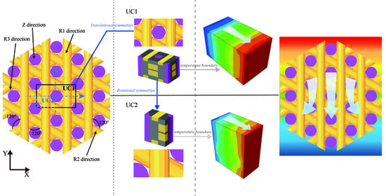
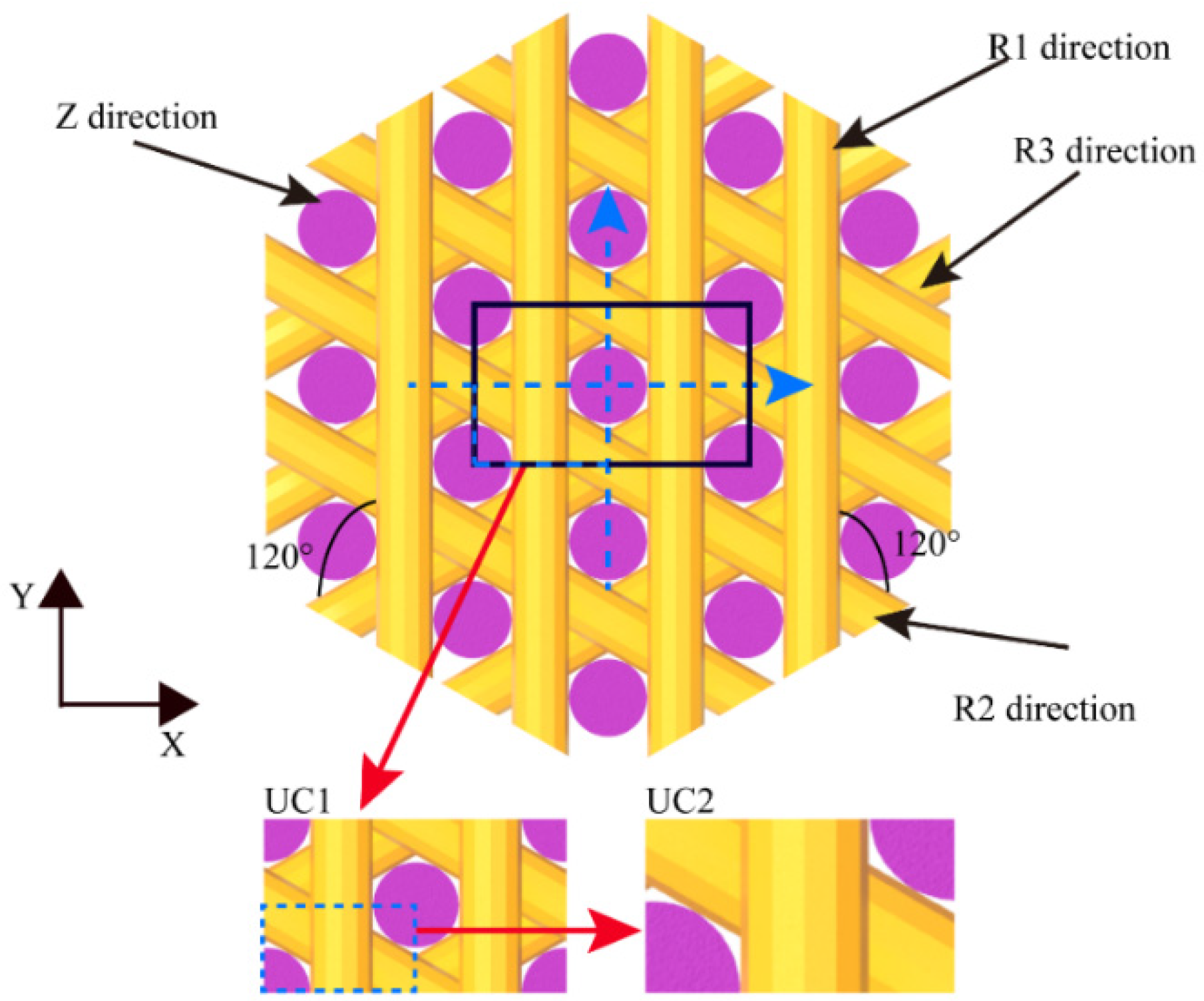
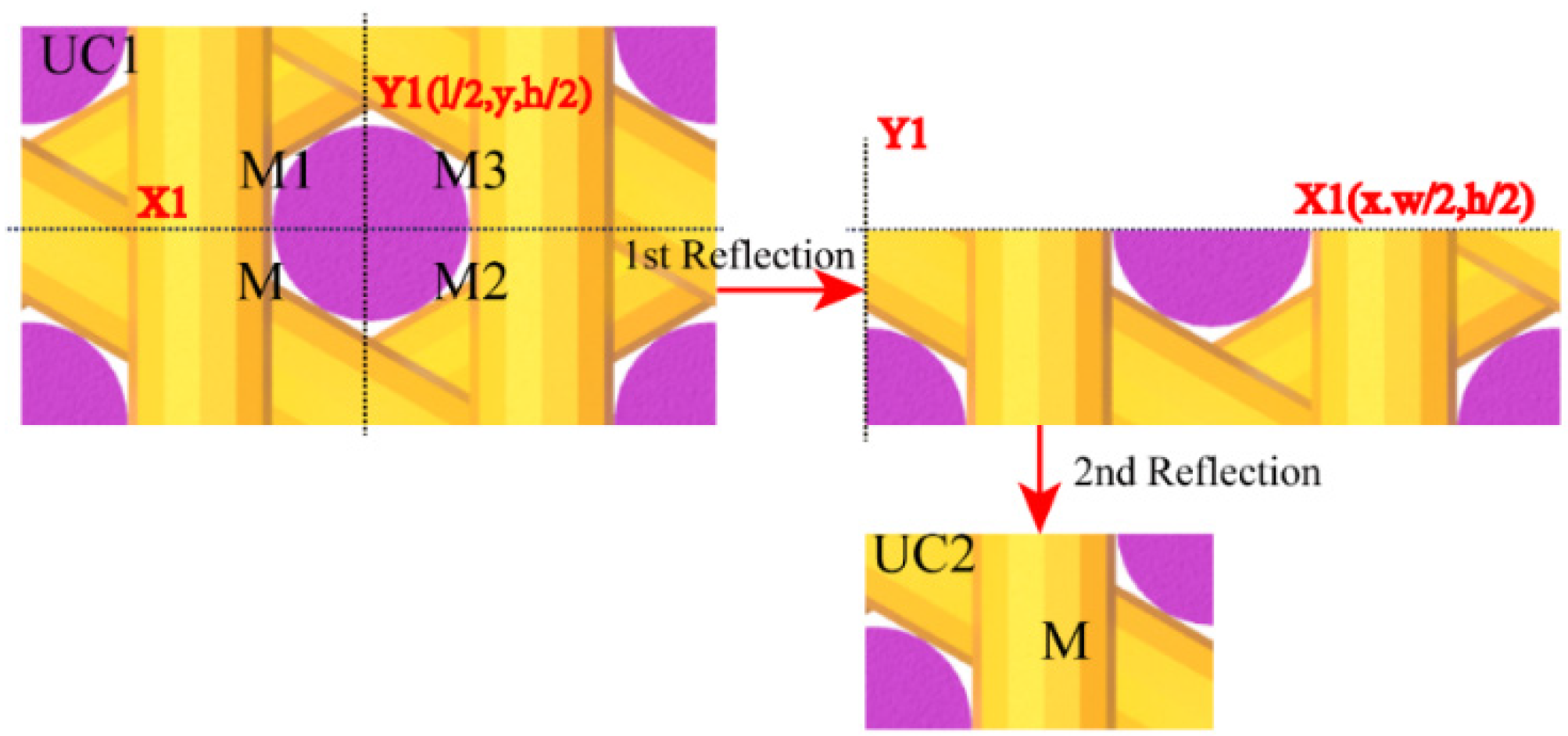
2.1. The Temperature and Heat Flux of Unit Cells Formed by 180° Rotational Symmetry

$M$ is an arbitrary node in the cube in Figure 4. The z-axis is defined as the axis of rotation. The left half of the cube would completely coincide with the right half if it rotates 180° around the z-axis, and $M=(x_1,y_1,z_1)$ can be converted to the node $M’=(-x_1,-y_1,z_1)$. As shown in Figure 4, a smaller-size unit cell is constructed using a 180° rotational transformation, by the domain $0\le x\le l/2$, $0\le y\le w$, $0\le z\le h$. Considering the relationship between the direction of heat flux and the rotation axis (z-axis), it can be divided into two categories: (1) antisymmetric thermal stimulus, which means that the heat flux is perpendicular to the axis of rotation in Figure 4, (2) symmetric thermal stimulus, which means the heat flux is parallel to the axis of rotation in Figure 5.

Based on the discussion above, the heat flux distributions and temperature relations of antisymmetric thermal stimulus and symmetric thermal stimulus can be depicted by Equations (1) and (2), respectively.

$$\begin{gathered} T_M-T_O=T_O-T_{M’}, \\ {q}_{x|M}=q_{x|M’}, \end{gathered}$$

(1)

$$\begin{gathered} T_M-T_O=T_{M’}-T_O, \\ {q}_{x|M}=q_{x|M’}, \end{gathered}$$

(2)

where, $T_M$, etc., is the temperature of the nodes in the cube, $q_{x|M}$, etc., is the heat flux of the nodes in x direction. It should be mentioned that the temperature of the node will be represented by the subscript of its coordinates in the following discussion. When describing the heat flux of the node, the left side of the subscript represents the direction of heat flow, and the right side represents the position of the node.

2.2. The Temperature Boundary Conditions of UC1

The temperature boundary conditions of the composites can be derived by the displacement boundary conditions proposed by Xia et al. [39], combining the homogenization theory and Fourier’s law of thermal conduction. As for calculating the effective thermal conductivity in x direction, ${\lambda }_{\mathrm{xx}}$, the heat flux $q_x$ and temperature gradient $\nabla T_{\mathrm{x}}$ of the two sides on the unit cell need to be acquired first. The $\nabla T_{\mathrm{x}}$ is a specified value that is prescribed by the equation $\nabla T_x=\Delta T/l$ in this work. The results of heat flux are acquired in the post-processing. In this work, $\Delta T=300k$ is prescribed when predicting the thermal conductivities of UC1 and UC2. For calculating ${\lambda }_{\mathrm{yy}}$ and ${\lambda }_{\mathrm{zz}}$, $\nabla T_y=\Delta T/w$ and $\nabla T_z=\Delta T/h$ can be used, respectively. After determining the temperature gradient, the temperature boundary conditions should be used for the UC1. The temperature boundary conditions in the x direction can be described as [26]:

$$T_{(l,y_1,z_1)}-T_{(0,0,0)}=\nabla T_x, T_{(x_1,w,z_1)}-T_{(0,0,0)}=0, T_{(x_1,y_1,h)}-T_{(0,0,0)}=0,$$

(3)

where $x_1$, $y_1$, $z_1$ are arbitrary values in x-axis, y-axis, and z-axis, respectively. The heat flux and temperature of the face, edge and node are expressed by a subscript of its coordinates in the following discussion.

Similarly, the temperature boundary conditions in the $y$ direction and $z$ direction can be described as Equations (4) and (5).

$$T_{(l,y_1,z_1)}-T_{(0,0,0)}=0, T_{(x_1,w,z_1)}-T_{(0,0,0)}=\nabla T_y, T_{(x_1,y_1,h)}-T_{(0,0,0)}=0,$$

(4)

$$T_{(l,y_1,z_1)}-T_{(0,0,0)}=0, T_{(x_1,w,z_1)}-T_{(0,0,0)}=0, T_{(x_1,y_1,h)}-T_{(0,0,0)}=\nabla T_z.$$

(5)

Equations (3)–(5) are the temperature boundary conditions of the UC1. UC2 is constructed from UC1 by rotational transformations, so the boundary conditions of UC2 need to be derived on the basis of UC1. The derivations of the temperature boundary conditions of UC2 are discussed in detail in the following section. It should be noted that deriving the temperature boundary conditions of UC2 also need to consider three conditions: (1) the temperature gradient $\nabla T_x$ when calculating the ${\lambda }_{xx}$, (2) the temperature gradient $\nabla T_y$ when calculating the ${\lambda }_{yy}$, (3) the temperature gradient $\nabla T_z$ when calculating the ${\lambda }_{zz}$.

2.3. The Temperature Boundary Conditions of UC2

In Figure 6, UC2 is obtained by two 180° rotational transformations of UC1. The sequence of the two rotations has no effect on the results. As shown in Figure 6 and Figure 7, the first 180° rotational conversion to construct the UC2 is around the X1 axis (line $(x,w/2,h/2)$), and the second 180° rotational conversion is around the Y1 axis (line $(l/2,y,h/2)$). Finally, UC2 is constructed, which is only a quarter of the size of UC1. As seen in the Figure 6, any node $M=(x_1,y_1,z_1)$ can be transformed from the corresponding nodes in the other three regions, namely $M1=(x_1,w-y_1,h-z_1)$, $M2=(l-x_{1,}{y}_1,h-z_1)$, and $M3=(l-x_1,w-y_1,z_1)$. Two sets of new boundary planes are formed by the two rotational transformations. The first set of boundary planes are $((0,l/2),0,z)$ and $((0,l/2),w/2,z)$, which are generated after the first rotational transformation. The second rotational transformation constructs UC2 with another set of boundary planes, which are $(0,(0,w/2),z)$ and $(l/2,(0,w/2),z)$. Both sets of new boundary planes need to derive the appropriate temperature boundary conditions.

Since the set of boundary planes formed by the first rotational transformation and the second rotational transformation are perpendicular to each other, the temperature gradient imposed on UC1 may become the different thermal stimulus for the two new sets. For instance, if the temperature gradient act on the x-axis, the heat flux may be perpendicular to plane $(0,(0,w/2),z)$ and plane $(l/2,(0,w/2),z)$, but parallel to plane $((0,l/2),0,z)$ and plane $((0,l/2),w/2,z)$. Thus, the temperature boundary conditions applicable to the two groups of boundary planes are different.

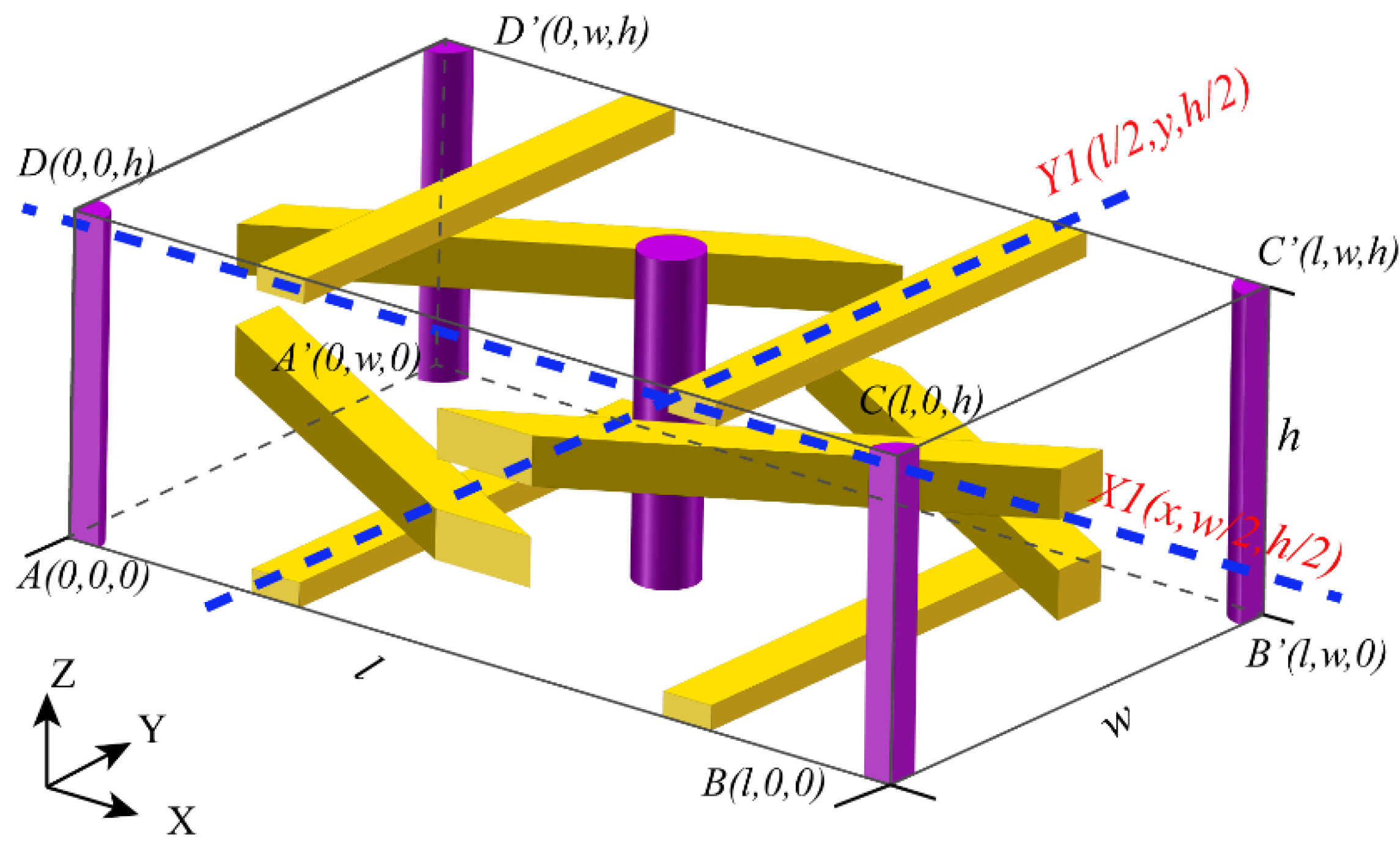
2.3.1. Boundary Conditions for Calculating ${\lambda }_{xx}$ of UC2

The temperature applied to UC2 is converted from the temperature boundary conditions acted on UC1 based on the pattern of rotational symmetries. When calculating the ${\lambda }_{xx}$ of UC1, the temperature boundary conditions are shown in Equation (3). When calculating the effective thermal conductivity in x direction of UC2, the planes $((0,l/2),0,z)$ and $((0,l/2),w/2,z)$ are parallel to x direction. The heat flux can be regarded as symmetric thermal stimulus. However, the heat flux on planes $(0,(0,w/2),z)$ and $(l/2,(0,w/2),z)$ need to be processed as an antisymmetric thermal stimulus.

Boundary Conditions of $((0,l/2),0,z)$ and $((0,l/2),w/2,z)$

By assuming an arbitrary node $M=(x_1,0,z_1)$ situated on the plane $((0,l/2),0,z)$, the temperature of $M$ is depicted as $T_{(x_1,0,z_1)}$, and the heat flux of $M$ is expressed as $q_{y|(x_1,0,z_1)}$. Similarly, the temperature and heat flux of $M1=(x_1,w,h-z_1)$ can be represented by $T_{(x_1,w,h-z_1)}$ and $q_{y|(x_1,w,h-z_1)}$, respectively, which is the corresponding node of $M$ for the first rotational transformation. Through Equations (3) and (2), the temperature boundary conditions of plane $((0,l/2),0,z)$ can be expressed as:

$$\begin{gathered} T_{(x_1,0,z_1)}=T_{(}{}_{x_1,w,h-z_1)}, \\ {q}_y{{}_{|}}_{(x_1,0,z_1)}=q_y{{}_{|}}_{(x_1,w,h-z_1)}. \end{gathered}$$

(6)

In the same way, the temperature and the heat flux of $M=(x_1,w/2,z_1)$ should be represented by $T_{(x_1,w/2,z_1)}$ and $q_{y|(x_1,w/2,z_1)}$, when $M$ is located on the plane $((0,l/2),w/2,z)$. $M1=(x_1,w/2,h-z_1)$ should be represented by $T_{(x_1,w/2,h-z_1)}$ and $q_{y|(x_1,w/2,h-z_1)}$, respectively, which is the corresponding node of $M$ for the first rotational transformation in the plane $((0,l/2),w/2,z)$. So, the temperature boundary conditions of plane $((0,l/2),w/2,z)$ can be described as

$$\begin{gathered} T_{(x_1,w/2,z_1)}=T_{(x_1,w/2,h-z_1)}, \\ {q}_{y|(x_1,w/2,z_1)}=q_{y|(x_1,w/2,h-z_1)}. \end{gathered}$$

(7)

Boundary Conditions of $(0,(0,w/2),z)$ and $(l/2,(0,w/2),z)$

The temperature of $M=(0,y_1,z_1)$ can be expressed by $T_{(0,y_1,z_1)}$ and the heat flux of $M$ can be depicted as $q_x{{}_{|}}_{(0,y_1,z_1)}$, when the $M$ is on the plane $(0,(0,w/2),z_1)$. The temperature of $M2=(l,y_1,h-z_1)$ should be represented by $T_{(l,y_1,h-z_1)}$, and the heat flux of $M2$ can be expressed as $q_x{{}_{|}}_{(l,y_1,h-z_1)}$. The $M2$ is the corresponding node of the $M=(0,y_1,z_1)$ for the second rotational transformation. Since the heat flux is perpendicular to the plane $(0,(0,w/2),z)$, the antisymmetric thermal stimulus is formed. Referring to Equations (1) and (3), the temperature boundary conditions of plane $(0,(0,w/2),z)$ can be expressed as:

$$\begin{gathered} T_{(0,y_1,z_1)}+T_{(l,y_1,h-z_1)}=2T_{(0,0,0)}+\nabla T_x, \\ {q}_x{{}_{|}}_{(0,y_1,z_1)}=-q_x{{}_{|}}_{(l,y_1,h-z_1)}. \end{gathered}$$

(8)

In the same way, the temperature and the heat flux of $M=(l/2,y_1,z_1)$, when located on plane $(l/2,(0,w/2),z)$, should be represented by $T_{(l/2,y_1,z_1)}$ and $q_x{{}_{|}}_{(l/2,y_1,z_1)}$, respectively. The temperature and the heat flux of $M2=(l/2,y_1,h-z_1)$ can be expressed by $T_{(l/2,y_1,h-z_1)}$ and $q_x{{}_{|}}_{(l/2,y_1,h-z_1)}$, which is the corresponding node of $M=(l/2,y_1,z_1)$. Thus, the boundary conditions of planes $(l/2,(0,w/2),z)$ can be expressed as:

$$\begin{gathered} T_{(l/2,y_1,z_1)}+T_{(l/2,y_1,h-z_1)}=2T_{(0,0,0)}+\nabla T_x, \\ {q}_x{{}_{|}}_{(\mathrm{l}/2,y_1,z_1)}=-q_x{{}_{|}}_{(l/2,y_1,h-z_1)}. \end{gathered}$$

(9)

Based on Equations (6)–(9), the temperature boundary conditions of UC2 are acquired in x direction when calculating the ${\lambda }_{\mathrm{xx}}$. Considering the nodes located at the faces, the nodes and the edges [40], the separate equations are summarized as:

$$\begin{gathered} q_x{{}_{|}}_{(0,y_1,z_1)}=-q_x{{}_{|}}_{(l/2,y_1,z_1)}, \\ {T}_{(0,y_1,z_1)}-T_A=0, T_{(l/2,y_1,z_1)}+T_{(l/2,y_1,h-z_1)}-2T_A=\nabla T_x, \\ {T}_{(l/2,y_1,z_1)}-T_A=\nabla T_x/2 \\ {q}_z{{}_{|}}_{(x_1,y_1,0)}=-q_z{{}_{|}}_{(x_1,y_1,h)}=0, \\ {T}_{(x_1,y_1,0)}=T_{(x_1,y_1,h)}, \end{gathered}$$

$$\begin{gathered} T_{A=(0,0,0)}=T_{B=(\mathrm{l}/2,0,0)}=T_{C=(l/2,0,h)}=T_{D=(0,0,h)}, \\ {T}_{A’=(0,w/2,0)}=T_{B’=(l/2,w/2,0)}=T_{C’=(l/2,w/2,h)}=T_{D’=(0,w/2,h)}=T_{A=(0,0,0)}+\nabla T_x/2, \end{gathered}$$

$$\begin{gathered} T_{5=(x,w/2,0)}=T_{6=(x,w/2,h)}=T_{7=(x,0,h)}=T_{8=(x,0,0)}, \\ {T}_{1=(0,y,0)}=T_{2=(l/2,0,z)}=T_{3=(0,y,h)}=T_{4=(0,0,z)}=T_{A=(0,0,0)}, \\ {T}_{9=(l/2,y,0)}=T_{10=(l/2,w/2,h)}=T_{11=(l/2,y,h)}=T_{12=(0,w/2,z)}=T_{A=(0,0,0)}+\nabla T_x/2. \end{gathered}$$

(10)

As shown in Figure 8, a new cube is constructed and used to describe the boundary conditions for UC2 derived in this article. The coordinate of $A$ is specified as $(0,0,0)$. Equation (10) are used to constraint the temperature boundary conditions of faces, vertices and edges, respectively. As shown in Equation (10), the faces of UC2 are sorted to three sets by x, y and z direction, respectively. The vertices of UC2 are classified into two sets by x-coordinate. The edges of UC2 are categorized into three sets according to their directions in Equation (10).

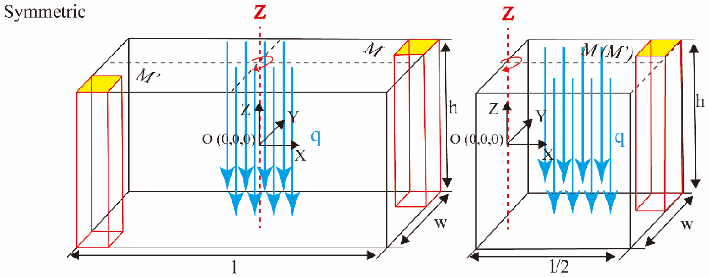
2.3.2. Boundary Conditions for Calculating ${\lambda }_{yy}$ of UC2

Equation (4) is the temperature boundary conditions for UC1 to calculate ${\lambda }_{yy}$. In order to predict the ${\lambda }_{yy}$ of UC2, the temperature boundary conditions that are suitable for UC2 need to be derived from UC1. The heat flux on the planes $((0,l/2),0,z)$ and $((0,l/2),w/2,z)$ can be regarded as antisymmetric thermal stimulus when imposing a temperature gradient in the y direction of UC2, while the heat flux on the planes $(0,(0,w/2),z)$ and $(l/2,(0,w/2),z)$ can be regarded as symmetric thermal stimulus. According to Equations (1), (2) and (4), the temperature boundary conditions for calculating ${\lambda }_{yy}$ of UC2 can be represented by:

$$\begin{gathered} q_x{{}_{|}}_{(0,y_1,z_1)}=-q_x{{}_{|}}_{(l/2,y_1,z_1)}=0, \\ {T}_{(l/2,y_1,z_1)}=T_{(l/2,y_1,h-z_1)}, T_{(0,y_1,z_1)}=T_{(}{}_{l/2,y_1,z_1)}, \\ {q}_{y|(x_1,0,z_1)}=-q_{y|(x_1,w/2,z_1)}, \\ {T}_{(x_1,0,z_1)}-T_A=0, T_{(x_1,w/2,z_1)}+T_{(x_1,w/2,h-z_1)}-2T_A=\nabla T_y, ,T_{(x_1,w/2,z_1)}-T_A=\nabla T_y/2, \\ {q}_z{{}_{|}}_{(x_1,y_1,0)}=-q_z{{}_{|}}_{(x_1,y_1,h)}=0, \\ {T}_{(x_1,y_1,0)}=T_{(x_1,y_1,h)}, \end{gathered}$$

$$\begin{gathered} T_{A=(0,0,0)}=T_{D=(0,0,h)}=T_{D’=(0,w/2,h)}=T_{A’=(0,w/2,0)}, \\ {T}_{B=(l/2,0,0)}=T_{B’=(l/2,w/2,0)}=T_{C’=(l/2,w/2,h}{}_{)}=T_{C=(l/2,0,h)}=T_{A=(0,0,0)}+\nabla T_y/2, \end{gathered}$$

$$\begin{gathered} T_{1=(0,y,0)}=T_{3=(0,y,h)}=T_{11=(l/2,y,h)}=T_{9=(l/2,y,0)}, \\ {T}_{5=(x,w/2,0)}=T_{6=(x,w/2,h)}=T_{10=(l/2,w/2,z)}=T_{2=(l/2,0,z)}=T_{A=(0,0,0)}+\nabla T_y/2, \\ {T}_{4=(0,0,z)}=T_{8=(0,y,0)}=T_{12=(0,w/2,z)}=T_{7=(0,y,h)}=T_{A=(0,0,0)}. \end{gathered}$$

(11)

2.3.3. Boundary Conditions for Calculating ${\lambda }_{zz}$ of UC2

The heat flux on the planes $(0,(0,w/2),z)$, $(l/2,(0,w/2),z)$, $((0,l/2),0,z)$, and $((0,l/2),w/2,z)$ can all be regarded as antisymmetric thermal stimulus when imposing a temperature gradient in the z direction. According to Equations (1) and (5), the temperature boundary conditions for calculating ${\lambda }_{zz}$ of UC2 can be represented by:

$$\begin{gathered} q_x{{}_{|}}_{(0,y_1,z_1)}=-q_x{{}_{|}}_{(l/2,y_1,z_1)}=0, \\ {T}_{(l/2,y_1,z_1)}+T_{(l/2,y_1,z_1)}-T_{A=(0,0,0)}=\nabla T_z, T_{(x_1,w/2,0)}-T_A=0, \\ {q}_y{{}_{|}}_{(x_1,0,z_1)}=-q_y{{}_{|}}_{(x_1,w/2,z_1)}=0, \\ {T}_{(0,w/2,z_1)}+T_{(0,w/2,h-z_1)}-T_A{}_{=(0,0,0)}=\nabla T_z, T_{(l/2,y_1,0)}-T_A=0, \\ {q}_z{{}_{|}}_{(x_1,y_1,0}{}_{)}=-q_z{{}_{|}}_{(x_1,y_1,h)}, \\ {T}_{(x_1,y_1,h)}-T_{(x_1,y_1,0)}=\nabla T_z, \end{gathered}$$

$$\begin{gathered} T_{A=(0,0,0)}=T_{B=(l/2,0,0)}=T_{B’=(l/2,w/2,0)}=T_{A’=(0,w/2,0)}, \\ {T}_{D=(0,0,h)}=T_{C=(l/2,0,h)}=T_{C’=(l/2,w/2,h)}=T_{D’=(0,w/2,h)}=T_{A=(0,0,0)}+\nabla T_z, \end{gathered}$$

$$\begin{gathered} T_{4=(0,0,z)}=T_{2=(l/2,0,z)}=T_{10=(l/2,w/2,z)}=T_{12=(0,w/2,z)}, \\ {T}_{1=(0,y,0)}=T_{5=(x,w/2,0)}=T_{9=(l/2,y,0)}=T_{8=(0,y,0)}=T_{A=(0,0,0)}, \\ {T}_{3=(0,y,h)}=T_{6=(x,w/2,h)}=T_{11=(l/2,y,h)}=T_{7=(0,y,h)}=T_{A=(0,0,0)}+\nabla T_z. \end{gathered}$$

(12)

As mentioned above, the temperature boundary conditions used to calculate the thermal conductivities of UC2 have been derived. Before predicting the effective thermal conductivities of 4D C/C composites, the thermal conductivities of carbon fiber rods and carbon fiber bundles need to be calculated first. Then, the results are taken as the input to calculate the thermal conductivities of 4D C/C composites.

3. Finite Element Analyses

3.1. Governing Equation of the Thermal Conduction

In this paper, the finite element analyses were operated on commercially available finite element software package ABAQUS/Standard (ver. 2016) under the environment of the operation system Windows. The finite element analysis of carbon fiber rods, carbon fiber bundles, and unit cells were run in steady-state conditions. The temperature difference is set on the models in the pre-processing, and heat flux throughout the model is acquired in the post-processing. The governing equation used for steady-state conditions is represented as:

$$\begin{array}{l}{\lambda }_{xx}\frac{{\partial }^{2}T}{\partial x^2}+{\lambda }_{yy}\frac{{\partial }^{2}T}{\partial y^2}+{\lambda }_{zz}\frac{{\partial }^{2}T}{\partial z^2}+({\lambda }_{xy}+{\lambda }_{yx})\frac{{\partial }^{2}T}{\partial x\partial y}+({\lambda }_{xz}+{\lambda }_{zx})\frac{{\partial }^{2}T}{\partial x\partial z}\\ +({\lambda }_{yz}+{\lambda }_{zy})\frac{{\partial }^{2}T}{\partial y\partial z}=0\end{array},$$

(13)

where ${\lambda }_{\mathrm{xx}}$, etc., are the thermal conductivities of the materials in Equation (13), and $T$ is the temperature. According to Equation (14), the thermal conductivities in the x, y, and z direction of the composites can be calculated after setting the thermal conductivities of the matrix and the reinforcement.

$$q=-\lambda \nabla T/d,$$

(14)

where $\nabla T$ is the temperature difference that is imposed in the pre-processing, $d$ is the distance between the two faces to which the temperature difference is imposed, $\lambda$ is the effective thermal conductivities of the composites that we want to acquire, and $q$ is the heat flux in the specified direction that can be obtained in the post-processing by Equation (15):

$$q=Q/A,$$

(15)

where $Q$ is the sum of the heat flux of the surface in x, y or z direction, and $A$ is the area of the surface in the same direction.

3.2. Material Properties

The properties of carbon fiber rods, carbon fiber bundles, and matrix are essential for predicting the thermodynamic performances of 4D C/C composites. The PAN-based fibers can be regard as transverse isotropic material, the thermal conductivity is higher in longitudinal direction than in transverse direction. The resin matrix is generally considered to be isotropic in thermal conductivities. However, as for pitch-derived matrix, the thermal conductivity in longitudinal direction is higher than the transverse direction [27,41].

Based on the manufacturing process, carbon fiber rods, carbon fiber bundles and matrix pocket are the three components that construct the 4D C/C composites. Carbon fiber rods are manufactured by pultrusion of carbon fiber and epoxy resin. The carbon fiber bundles are made by carbon fiber and pitch. The fiber volume fractions of carbon fiber rods and carbon fiber bundles are 80% and 57%, respectively [27]. The matrix pocket is regard as disordered graphite, because of the high temperature graphitization treatment. The thermal conductivities of all ingredients that construct 4D C/C composites are shown in

Table 1. Thermal conductivities of the constituent materials.

Material/Heat Treating Temperature	Thermal Conductivity/(W∙m−1∙K−1)
	Transverse	Circumferential	Longitudinal
T300 fiber/PAN 2673 K	0.76	0.76	76
Resin based Matrix 2673 K	64.3	64.3	64.3
Pitch based Matrix 2673 K	0.64	64.3	257
Disordered Graphite	110	110	110

, and the properties are adopted from the literature [27,42].

3.3. Thermal Conductivities of Carbon Fiber Rods and Carbon Fiber Bundles

The geometry models of carbon fiber rods and carbon fiber bundles were directly built in ABAQUS. It should be noted that the temperature gradient was prescribed to be 25 K rather than 300 K when calculating the thermal conductivities of carbon fiber rod and carbon fiber bundle. In general, carbon fiber rods and carbon fiber bundles can both be regarded as transverse isotropic composites. The longitudinal thermal conductivity of transverse isotropic composites is usually calculated by classical mixture rule (Parallel Model). However, there is no uniform theoretical formula for the prediction of transverse thermal conductivities. There are quite a few differences in the results of the transverse thermal conductivities calculated by different formulas [43]. In this work, the Series Model, Charles Model [44], Pilling Model [45], and Maxwell Model [46] are used to calculate the transverse thermal conductivities, compared with results calculated by the FEM analysis. The temperature and heat flux distributions of carbon fiber rods and carbon fiber bundles are shown in Figure 9 and Figure 10, respectively. The numerical results are presented in

Table 2. Comparison of results by the FEM analysis and equations.

Model	Fiber Bundle/(W∙m−1∙K−1)		Fiber Rod/(W∙m−1∙K−1)
	Longitudinal Thermal Conductivity	Transverse Thermal Conductivity	Longitudinal Thermal Conductivity	Transverse Thermal Conductivity
Finite element analysis	149.24	11.33	73.74	3.89
Parallel Model	153.82		73.66
Series Model		1.32		0.95
Charles model		0.29		0.12
Pilling Model		13.08		3.88
Maxwell Model		18.14	73.74	7.71

.

$$\mathrm{Parallel} \mathrm{Model}: {\lambda }_{yl}={\lambda }_f{}_l{V}_f+{\lambda }_m(1-V_f),$$

(16)

$$\mathrm{Series} \mathrm{Model}: {\lambda }_{yt}=\frac{{\lambda }_{ft}{\lambda }_m}{{\lambda }_m{V}_f+{\lambda }_f{}_t(1-V_f)},$$

(17)

$$\mathrm{Charles} \mathrm{Model}: {\lambda }_{yt}=\frac{{\lambda }_m(1-V_f)+{\lambda }_f{}_t(1+V_f)}{{\lambda }_{ft}(1-V_f)+{\lambda }_m(1+V_f)},$$

(18)

$$\mathrm{Pilling} \mathrm{Model}: {\lambda }_{ft}=\frac{{\lambda }_m}{4}{\left[\sqrt{{(1-V_f)}^2{(\frac{{\lambda }_{ft}}{{\lambda }_m}-1)}^2+4\frac{{\lambda }_f{}_t}{{\lambda }_m}}-(1-V_f)(\frac{{\lambda }_f{}_t}{{\lambda }_m}-1)\right]}^2,$$

(19)

$$\mathrm{Maxwell} \mathrm{Model}: {\lambda }_{ft}={\lambda }_m\frac{{\lambda }_{ft}+2{\lambda }_m+2V_f({\lambda }_f{}_t-{\lambda }_m)}{{\lambda }_{ft}+2{\lambda }_m-2V_f({\lambda }_{ft}^{}-{\lambda }_m)},$$

(20)

where ${\lambda }_{yl}$, ${\lambda }_{yt}$, ${\lambda }_{fl}$, and ${\lambda }_f{}_t$ represent the thermal conductivities in the longitudinal direction of the yarn, in the transverse direction of the yarn, in the longitudinal direction of the fiber, and in the transverse direction of the fiber, respectively, $V_f$ is the fiber volume fraction of yarn, and ${\lambda }_m$ is the thermal conductivities of the matrix. As shown in Table 2, the calculated results of the parallel model in Equation (15) are close to the results of the numerical model in the longitudinal direction. However, there is a large error in the results calculated by the Series Model in Equation (16) and the Charles Model in Equation (17) in the transverse direction of yarn. The results predicted by Pilling model in Equation (18) are close to the results calculated by the FEM analysis.

Then, the thermal conductivities of carbon fiber bundles and carbon fiber rods calculated by FEM analysis and the parallel model are then used for predicting the effective thermal conductivities of 4D C/C composites.

3.4. Domain Discretization of UC1 and UC2

The geometry models of the UC1 and UC2 were established based on the CAE (computer-aided engineering) software SolidWorks (Version 2016, Dassault Systemes, Massachusetts, MA, USA, 2016). In this work, UC2 is one-fourth of the size of UC1. As seen in Figure 11, the UC1 is prescribed as a cube by the domain $0\le x\le l$, $0\le y\le w$, $0\le z\le h$. $l$ and $w$ are the length and width of the UC1, respectively, $h$ is the height of UC1 and UC2, $d_{fr}$ is the diameter of carbon fiber rod, $h_{fb}$ and $l_{fb}$ represent the height and length of carbon fiber bundle, respectively, and $g$ is the distance between the carbon fiber bundle and the carbon fiber rod. For the unit cells discussed above, these parameters are fixed as follows, $l=5.54 \mathrm{mm}$, $w=3.2 \mathrm{mm}$, $h=3.3 \mathrm{mm}$, $d_{fr}=1.2 \mathrm{mm}$, $h_{fb}=0.9 \mathrm{mm}$, $l_{fb}=0.9 \mathrm{mm}$, $g=0.34 \mathrm{mm}$.

In addition, three additional diameters $(d_{fr}=1.4 \mathrm{mm}, 1.6 \mathrm{mm}, 1.8 \mathrm{mm})$ of carbon fiber rods are set in order to observe the effect of fiber rod diameter on the thermal conductivities while the value of $g$ is fixed. As discussed above, the thermal conductivities of carbon fiber bundles and carbon fiber rods are used as inputs for calculating the thermal conductivities of 4D C/C composites, so local coordinates are required to define the axes of carbon fiber bundles and carbon fiber rods. UC1 and UC2 are both meshed by the C3D8R element, which imposed the temperature boundary conditions discussed in Section 2.2 and Section 2.3, respectively. The meshed models of UC1 and UC2 can be seen in Figure 11, and the corresponding number of elements of the two-unit cells with carbon fiber rods of different diameters are shown in

Table 3. The number of elements of UC1 and UC2 with carbon fiber rods of different diameters.

Diameter of the Fiber Rods	The Size of Unit Cell
	The Number of Elements of UC1	The Number of Elements of UC2
1.2 mm	734,448	184,276
1.4 mm	841,896	211,464
1.6 mm	971,520	243,672
1.8 mm	1,112,496	273,240

.

4. Results and Discussion

Figure 12 shows the temperature distributions of the two models when calculating the ${\lambda }_{xx}$ $(d_{fr}=1.2 \mathrm{mm})$. The result shows a relatively uniform temperature distribution for two-unit cells. The temperature of $T_A{}_{=(0,0,0)}$ are both set to 0 K in UC1 and UC2. In order to compare the temperature distributions obtained by the two models, temperature on the lines $X1=(x,w/2,h/2)$ and $Y1=(l/2,y,h/2)$ for the two models are extracted. As can be seen in Figure 13, the values of temperature in lines $X1$ and $Y1$ of UC1 and UC2 are the almost equal. These results suggest that the temperature boundary conditions imposed on UC2 are accurate.

Figure 14 shows the heat flux distributions used to calculate the ${\lambda }_{xx}$ of UC1 and UC2 $(d_{fr}=1.2 \mathrm{mm})$, respectively. The results in Figure 14 can indicate that the heat flux in the matrix region is higher than other regions because the matrix has the higher thermal conductivities in the x direction. In addition, the heat flux distributions of UC1 and UC2 are extraordinarily similar.

The measured thermal conductivities of the UC1 and UC2 are shown in

Table 4. Comparison of the FE results with the experimental results in [27].

		Thermal Conductivity (W·m−1·k−1)
Direction		Experimental Values in [27]	UC1	UC2
Transverse	X	75.2	79.82	80.13
	Y		81.10	81.89
Longitudinal	Z	58.73	63.01	62.61

with the fiber rod diameter of 1.2 mm. The predicted values in transverse are 5.8 to 8.2% and longitudinal 6.2 to 6.8% both higher than the experimental values in [27].

The effect of carbon fiber rods with different diameters on the effective thermal conductivities of 4D C/C composites is shown in Figure 15. The transverse thermal conductivities (${\lambda }_{xx}$, ${\lambda }_{yy}$) predicted by UC1 are both higher than the results predicted by UC2 slightly. However, the longitudinal thermal conductivity (${\lambda }_{zz}$) predicted by UC1 is always slightly smaller than that of UC2. In addition, it can be easily found that the longitudinal thermal conductivity of the 4D C/C composites increases as the diameter of the fiber rods increase, while the effective transverse thermal conductivities decrease.

According to the discussions above, the heat flux and temperature distributions at the corresponding positions of the two-unit cells are both almost the same. The correctness of the temperature boundary conditions imposed on the UC2 derived from the boundary conditions of UC1 is verified. The UC2 can be used to predict the thermal conductivities of 4D C/C composites, which is constructed by two 180° rotational symmetry transformations of UC1. The smaller-size model can greatly save computing time and computing resources. In this work, the computational time (including the pre-processing, solving and post-processing) of UC2 is about only 32.9% of UC1.

5. Conclusions

In this work, the thermal conductivities of 4D C/C composites are predicted by UC1 and UC2, where UC2 is constructed by two 180° rotational transformations of UC1, and its volume is a quarter of UC1. According to the equations of temperature relations derived from 180° rotational transformation in Section 2.1 and the temperature boundary conditions imposed on UC1, the temperature boundary conditions of UC2 are derived. The accuracy of the imposed boundary conditions in UC2 is verified when compared the temperature and heat flux at the specific positions of UC1 and UC2. The thermal conductivities of 4D C/C composites calculated by UC1 and UC2 are compared with the experimental values in [27]. The results in transverse direction predicted by UC1 and UC2 are both higher than experimental values, which are 5.8 to 6.2% and 7.3 to 8.2%, respectively. In longitudinal direction, the measured results of UC1 and UC2 are 6.8% and 6.2% higher than the experimental results, respectively.

According to the results calculated in the above, two conclusions can be drawn:

In general, the unit cells are constructed by translational transformation used to predict the thermal conductivities of 4D C/C composites. However, a smaller-size unit cell (UC2) is proposed by two $180°$ rotational transformations based on UC1 in this work. They can both predict the thermal conductivities of 4D C/C composites accurately. The smaller-size unit cell can save computing time and computing resources greatly.

The carbon fiber rods with different diameters have an impact on the effective thermal conductivities of 4D C/C composites. The longitudinal thermal conductivity of the 4D C/C composites increases as the diameter of the fiber rods increase, while the transverse thermal conductivities decrease.

References

1. Hui, W.H.; Bao, F.T.; Wei, X.G.; Liu, Y. Analysis of Ablative Performance of C/C Composite Throat Containing Defects Based on X-ray 3D Reconstruction in a Solid Rocket Motor. Int. J. Turbo. Jet-Engines 2015, 32, 351–359. [Google Scholar] [CrossRef]
2. Ozcan, S.; Tezcan, J.; Filip, P. Microstructure and elastic properties of individual components of C/C composites. Carbon 2009, 47, 3403–3414. [Google Scholar] [CrossRef]
3. Zaman, W.; Li, K.-Z.; Li, W.; Zaman, H.; Ali, K. Flexural strength and thermal expansion of 4D carbon/carbon composites after flexural fatigue loading. N. Carbon Mater. 2014, 29, 169–175. [Google Scholar] [CrossRef]
4. Li, B.-L.; Guo, J.-G.; Xun, B.; Xu, H.-T.; Dong, Z.-J.; Li, X.-K. Preparation, microstructure and properties of three-dimensional carbon/carbon composites with high thermal conductivity. N. Carbon Mater. 2020, 35, 567–575. [Google Scholar] [CrossRef]
5. Mierzwiczak, M.; Kolodziej, J.A. The inverse determination of volume fraction of fibres in reinforced composite with imperfect thermal contact between constituents. J. Theor. Appl. Mech. 2011, 49, 987–1001. [Google Scholar]
6. Franco, A. An apparatus for the routine measurement of thermal conductivity of materials for building application based on a transient hot-wire method. Appl. Therm. Eng. 2007, 27, 2495–2504. [Google Scholar] [CrossRef]
7. Gustafsson, S.E. Transient plane source techniques for thermal-conductivity and thermal-diffusivity measurements of solid materials. Rev. Sci. Instrum. 1991, 62, 797–804. [Google Scholar] [CrossRef]
8. Jiang, C.P.; Chen, F.L.; Yan, P.; Song, F. A four-phase confocal elliptical cylinder model for predicting the effective thermal conductivity of coated fibre composites. Philos. Mag. 2010, 90, 3601–3615. [Google Scholar] [CrossRef] [Green Version]
9. Sihn, S.; Roy, A.K. Micromechanical analysis for transverse thermal conductivity of composites. J. Compos. Mater. 2011, 45, 1245–1255. [Google Scholar] [CrossRef]
10. Mierzwiczak, M.; Kolodziej, J.A. The inverse determination of the volume fraction of fibers in a unidirectionally reinforced composite for a given effective thermal conductivity. J. Mech. Mater. Struct. 2012, 7, 229–238. [Google Scholar] [CrossRef] [Green Version]
11. Mierzwiczak, M.; Kolodziej, J.A. The inverse determination of the thermal contact resistance components of unidirectionally reinforced composite. Inverse Probl. Sci. Eng. 2013, 21, 283–297. [Google Scholar] [CrossRef]
12. Asif, M.; Tariq, A.; Singh, K.M. Estimation of thermal contact conductance using transient approach with inverse heat conduction problem. Heat Mass Transf. 2019, 55, 3243–3264. [Google Scholar] [CrossRef]
13. Marcos-Gomez, D.; Ching-Lloyd, J.; Elizalde, M.R.; Clegg, W.J.; Molina-Aldareguia, J.M. Predicting the thermal conductivity of composite materials with imperfect interfaces. Compos. Sci. Technol. 2010, 70, 2276–2283. [Google Scholar] [CrossRef] [Green Version]
14. Li, X.; Xing, L.X.; Zheng, K.L.; Wei, P.; Du, L.F.; Shen, M.W.; Shi, X.Y. Formation of Gold Nanostar-Coated Hollow Mesoporous Silica for Tumor Multimodality Imaging and Photothermal Therapy. ACS Appl. Mater. Interfaces 2017, 9, 5817–5827. [Google Scholar] [CrossRef] [PubMed]
15. Gou, J.J.; Dai, Y.J.; Li, S.G.; Tao, W.Q. Numerical study of effective thermal conductivities of plain woven composites by unit cells of different sizes. Int. J. Heat Mass Transf. 2015, 91, 829–840. [Google Scholar] [CrossRef]
16. Jiang, L.L.; Xu, G.D.; Cheng, S.; Lu, X.M.; Zeng, T. Predicting the thermal conductivity and temperature distribution in 3D braided composites. Compos. Struct. 2014, 108, 578–583. [Google Scholar] [CrossRef]
17. Dong, K.; Zhang, J.J.; Cao, M.; Wang, M.L.; Gu, B.H.; Sun, B.Z. A mesoscale study of thermal expansion behaviors of epoxy resin and carbon fiber/epoxy unidirectional composites based on periodic temperature and displacement boundary conditions. Polym. Test 2016, 55, 44–60. [Google Scholar] [CrossRef] [Green Version]
18. Ning, Q.G.; Chou, T.W. Closed-form solutions of the inpalne effective thermal-conductivities of woven-fabric composites. Compos. Sci. Technol. 1995, 55, 41–48. [Google Scholar] [CrossRef]
19. Ning, Q.G.; Chou, T.W. A general analytical model for predicting the transverse effective thermal conductivities of woven fabric composites. Compos. Part A Appl. Sci. Manuf. 1998, 29, 315–322. [Google Scholar] [CrossRef]
20. Tu, Z.C.; Mao, J.K.; Han, X.S.; He, Z.Z. Prediction Model for the Anisotropic Thermal Conductivity of a 2.5-D Braided Ceramic Matrix Composite with Thin-Wall Structure. Appl. Sci. Basel 2019, 9, 875. [Google Scholar] [CrossRef] [Green Version]
21. Gou, J.J.; Fang, W.Z.; Dai, Y.J.; Li, S.G.; Tao, W.Q. Multi-size unit cells to predict effective thermal conductivities of 3D four-directional braided composites. Compos. Struct. 2017, 163, 152–167. [Google Scholar] [CrossRef]
22. Liu, Y.; Qu, Z.G.; Guo, J.; Zhao, X.M. Numerical study on effective thermal conductivities of plain woven C/SiC composites with considering pores in interlaced woven yarns. Int. J. Heat Mass Transf. 2019, 140, 410–419. [Google Scholar] [CrossRef]
23. Ming, X.L.; Chen, H.T.; Wang, D.H. Optimization of Processing Parameters to Increase Thermal Conductivity of Rice Straw Fiber Film. Appl. Sci. Basel 2019, 9, 4645. [Google Scholar] [CrossRef] [Green Version]
24. Sun, Z.; Shan, Z.D.; Shao, T.M.; Zhang, Q. Numerical analysis of out-of-plane thermal conductivity of C/C composites by flexible oriented 3D weaving process considering voids and fiber volume fractions. J. Mater. Res. 2020, 35, 1888–1897. [Google Scholar] [CrossRef]
25. Gou, J.J.; Ren, X.J.; Fang, W.Z.; Li, S.G.; Tao, W.Q. Two small unit cell models for prediction of thermal properties of 8-harness satin woven pierced composites. Compos. Part B Eng. 2018, 135, 218–231. [Google Scholar] [CrossRef]
26. Li, H.Z.; Li, S.G.; Wang, Y.C. Prediction of effective thermal conductivities of woven fabric composites using unit cells at multiple length scales. J. Mater. Res. 2011, 26, 384–394. [Google Scholar] [CrossRef]
27. Wei, K.L.; Li, J.; Shi, H.B.; Tang, M. Two-Scale Prediction of Effective Thermal Conductivity of 3D Braided C/C Composites Considering Void Defects by Asymptotic Homogenization Method. Appl. Compos. Mater. 2019, 26, 1367–1387. [Google Scholar] [CrossRef]
28. Alghamdi, A.; Alharthi, H.; Alamoudi, A.; Alharthi, A.; Kensara, A.; Taylor, S. Effect of Needling Parameters and Manufacturing Porosities on the Effective Thermal Conductivity of a 3D Carbon-Carbon Composite. Materials 2019, 12, 13. [Google Scholar] [CrossRef] [PubMed] [Green Version]
29. Lee, J.; Lee, H.I.; Paik, J.G. Thermal conductivities of a needle-punched carbon/carbon composite with unbalanced structures. Carbon Lett. 2020, 9. [Google Scholar] [CrossRef]
30. Penide-Fernandez, R.; Sansoz, F. Anisotropic thermal conductivity under compression in two-dimensional woven ceramic fibers for flexible thermal protection systems. Int. J. Heat Mass Transf. 2019, 145, 11. [Google Scholar] [CrossRef]
31. Islam, M.R.; Pramila, A. Thermal conductivity of fiber reinforced composites by the FEM. J. Compos. Mater. 1999, 33, 1699–1715. [Google Scholar] [CrossRef]
32. Li, S. General unit cells for micromechanical analyses of unidirectional composites. Composites Part A Appl. Sci. Manuf. 2001, 32, 815–826. [Google Scholar] [CrossRef]
33. Li, S.; Reid, S.R. On the symmetry conditions for laminated fiber-reinforced composite structures. Int. J. Solids Struct. 1992, 29, 2867–2880. [Google Scholar] [CrossRef]
34. Zhu, X.; Han, L.; Yang, F.; Jiang, J.; Jia, X.L. Lightweight mesoporous carbon fibers with interconnected graphitic walls for supports of form-stable phase change materials with enhanced thermal conductivity. Sol. Energy Mater. Sol. Cells 2020, 208, 11. [Google Scholar] [CrossRef]
35. Tanov, R.; Tabiei, A. Computationally efficient micromechanical models for woven fabric composite elastic moduli. J. Appl. Mech. Trans. ASME 2001, 68, 553–560. [Google Scholar] [CrossRef]
36. Lu, J.; Hao, K.; Liu, L.; Li, H.; Li, K.; Qu, J.; Yan, X. Ablation resistance of SiC-HfC-ZrC multiphase modified carbon/carbon composites. Corros. Sci. 2016, 103, 1–9. [Google Scholar] [CrossRef]
37. Li, X.; Xiong, Z.G.; Xu, X.Y.; Luo, Y.; Peng, C.; Shen, M.W.; Shi, X.Y. Tc-99m-Labeled Multifunctional Low-Generation Dendrimer-Entrapped Gold Nanoparticles for Targeted SPECT/CT Dual-Mode Imaging of Tumors. ACS Appl. Mater. Interfaces 2016, 8, 19883–19891. [Google Scholar] [CrossRef] [PubMed]
38. Li, S.; Zhou, C.; Yu, H.; Li, L. Formulation of a unit cell of a reduced size for plain weave textile composites. Comput. Mater. Sci. 2011, 50, 1770–1780. [Google Scholar] [CrossRef]
39. Xia, Z.H.; Zhang, Y.F.; Ellyin, F. A unified periodical boundary conditions for representative volume elements of composites and applications. Int. J. Solids Struct. 2003, 40, 1907–1921. [Google Scholar] [CrossRef]
40. Gou, J.-J.; Zhang, H.; Dai, Y.-J.; Li, S.; Tao, W.-Q. Numerical prediction of effective thermal conductivities of 3D four-directional braided composites. Compos. Struct. 2015, 125, 499–508. [Google Scholar] [CrossRef]
41. Li, X.; Lu, S.Y.; Xiong, Z.G.; Hu, Y.; Ma, D.; Lou, W.Q.; Peng, C.; Shen, M.W.; Shi, X.Y. Light-Addressable Nanoclusters of Ultrasmall Iron Oxide Nanoparticles for Enhanced and Dynamic Magnetic Resonance Imaging of Arthritis. Adv. Sci. 2019, 6, 9. [Google Scholar] [CrossRef] [PubMed] [Green Version]
42. Grujicic, M.; Zhao, C.L.; Dusel, E.C.; Morgan, D.R.; Miller, R.S.; Beasley, D.E. Computational analysis of the thermal conductivity of the carbon-carbon composite materials. J. Mater. Sci. 2006, 41, 8244–8256. [Google Scholar] [CrossRef]
43. Dong, K.; Zhang, J.; Jin, L.; Gu, B.; Sun, B. Multi-scale finite element analyses on the thermal conductive behaviors of 3D braided composites. Compos. Struct. 2016, 143, 9–22. [Google Scholar] [CrossRef] [Green Version]
44. Charles, J.; Wilson, D. A model of passive thermal nondestructive evaluation of composite laminates. Polym. Compos. 1981, 2, 105–111. [Google Scholar] [CrossRef] [Green Version]
45. Pilling, M.; Yates, B.; Black, M.; Tattersall, P. The thermal conductivity of carbon fibre-reinforced composites. J. Mater. Sci. 1979, 14, 1326–1338. [Google Scholar] [CrossRef]
46. Zhou, L.C.; Sun, X.H.; Chen, M.W.; Zhu, Y.B.; Wu, H.G. Multiscale modeling and theoretical prediction for the thermal conductivity of porous plain-woven carbonized silica/phenolic composites. Compos. Struct. 2019, 215, 278–288. [Google Scholar] [CrossRef]
Figure 1. Framework of the entire solving process.
Applsci 11 01171 g001
Figure 2. The formulation of UC1 and UC2.
Applsci 11 01171 g002
Figure 3. Topological relationship of the main yarns in UC1.
Applsci 11 01171 g003
Figure 4. The relations of the antisymmetric thermal stimulus from rotational transformation.
Applsci 11 01171 g004
Figure 5. The relations of the symmetric thermal stimulus from rotational transformation.
Applsci 11 01171 g005
Figure 6. The two rotational transformations of UC2 from UC1.
Applsci 11 01171 g006
Figure 7. UC1 and UC2 model of four-directional carbon/carbon (4D C/C) composites.
Applsci 11 01171 g007
Figure 8. Boundaries of UC2.
Applsci 11 01171 g008
Figure 9. Temperature and heat flux distributions of the carbon fiber bundle: (a) temperature, (b) heat flux.
Applsci 11 01171 g009
Figure 10. Temperature and heat flux distributions of the carbon fiber rod: (a) temperature, (b) heat flux.
Applsci 11 01171 g010
Figure 11. Meshed models of (a) UC1 and (b) UC2.
Applsci 11 01171 g011
Figure 12. Temperature distributions for the calculation of λ x x in UC1 and UC2.
Applsci 11 01171 g012
Figure 13. Temperature on lines (a) X1; (b) Y1.
Applsci 11 01171 g013
Figure 14. The distributions of heat flux for the calculation of λ x x in UC1 and UC2.
Applsci 11 01171 g014
Figure 15. The effective thermal conductivities of UC1 and UC2 with carbon fiber rods of different diameters.
Applsci 11 01171 g015