Shadow Estimation for Ultrasound Images Using Auto-Encoding Structures and Synthetic Shadows

Abstract

Acoustic shadows are common artifacts in medical ultrasound imaging. The shadows are caused by objects that reflect ultrasound such as bones, and they are shown as dark areas in ultrasound images. Detecting such shadows is crucial for assessing the quality of images. This will be a pre-processing for further image processing or recognition aiming computer-aided diagnosis. In this paper, we propose an auto-encoding structure that estimates the shadowed areas and their intensities. The model once splits an input image into an estimated shadow image and an estimated shadow-free image through its encoder and decoder. Then, it combines them to reconstruct the input. By generating plausible synthetic shadows based on relatively coarse domain-specific knowledge on ultrasound images, we can train the model using unlabeled data. If pixel-level labels of the shadows are available, we also utilize them in a semi-supervised fashion. By experiments on ultrasound images for fetal heart diagnosis, we show that our method achieved 0.720 in the DICE score and outperformed conventional image processing methods and a segmentation method based on deep neural networks. The capability of the proposed method on estimating the intensities of shadows and the shadow-free images is also indicated through the experiments.

1. Introduction

Ultrasound (US) imaging is a popular modality of medical imaging. It is the first choice of diagnostic imaging because of these advantages: (i) it is noninvasive and has no side effects like X-rays and computed tomography (CT), (ii) equipment for US is smaller and cheaper than that of CT and magnetic resonance imaging (MRI), and (iii) it has higher temporal resolution (typically around 10–100 frames per second [1]) than CT and MRI. US imaging is used for a wide range of medical fields [1]; typically it is employed to examine superficial organs, intra-abdominal organs, hearts, and fetuses. On the other hand, US imaging suffers from low spatial resolution (typically around 10 μm– 1 mm [2]) and artifacts. Resulting images are often very noisy, and small findings and structures can be difficult to see.

To alleviate noise in US images and to support diagnosis, a number of technologies have been proposed. Recent equipment for US imaging comes with several techniques to improve the quality of US images [3]. For example, emitting sound waves from multiple different angles [4] and utilizing low-frequency bands that are hard to attenuate [5]. From the perspective of image processing, image enhancement methods have also been proposed [6,7].

Despite these techniques, acoustic shadows [8] (hereinafter simply referred to as shadows) that are common artifacts in US images are problematic. Shadows are shown as dark areas in US images. They are mainly caused by bones and air which reflect or absorb US emitted by probes. We cannot retrieve information of the areas that US does not reach, and thus, the areas are dark and dimmed. In some senses, shadows can be features for making a diagnosis; comet-tail artifact is known as a feature for finding gallstones [9], for example. However, we focus on situations that we are interested in structures of the organs such as fetal heart diagnosis. Because the regions of shadows have less information than shadow-free areas, clinicians can hardly make the right diagnosis if target organs are covered by shadows in such situations. Moreover, such shadows can degrade the performance of the image recognition methods for US images [10,11,12,13,14,15] although they are advancing lately with the rise of deep neural networks (DNNs) [16]. The only way to fundamentally avoid shadows is to move the probes so that the sound waves do not run into the obstacles. Shadows are basically unavoidable, but detecting such shadows is useful for assessing the quality of US images; whether the images can be used for diagnosis or image recognition techniques. Especially, for computer-aided diagnosis systems that detect structures such as [17], shadows can be critical for its performance. If shadows are detected while the US images are taking, we can notify the examiners whether the quality of the images is adequate or instruct them to retake the images if needed. Hence, shadows themselves have almost no information, but detecting them is crucial.

In this paper, we propose a shadow estimation method based on auto-encoding structures [18], a form of DNNs. The auto-encoding structures are constructed and trained to encode input images to feature vectors, decode the feature into images of estimated shadows and images of estimated shadow-free input, and then combine them to reconstruct the input. The structures enable us to obtain estimated shadows and estimated clean images at the same time. The primal target of the method is to estimate shadows, and the estimated clean images are supplementary outputs. The method is trained to localize shadows and estimate their intensity (or brightness) rather than just segmenting them as a pixel-wise binary classification (i.e., segmentation). Estimating the intensity is novel and motivated by the fact that shadows are often semi-transparent. By knowing the intensities of shadows, we can ignore detected shadows if they have low intensities. Considering the semi-transparency of shadows, labeling is quite difficult because the correct intensity of shadows are unknown; even annotating binary labels is difficult because of the ambiguity and variety of shadows. To address this problem, we introduce synthetic shadows as pseudo labels. If the target and method of the examination are fixed (i.e., the domain of US images is fixed), we can get to know the possible shapes of shadows. Based on the prior knowledge, we generate and inject simulated shadows with random shapes and intensities into the images and make the method learn them. In this way, shadows with any intensity can be learned without giving labeled data. Additionally, we also utilize pixel-wise binary labels if available in a semi-supervised fashion. An algorithm that estimates the intensity of the labeled shadows is proposed and the labels are turned into semi-transparent ones. We applied the proposed method to US images for fetal heart diagnosis and evaluated the performance. As a segmentation method, our method outperformed previous methods based on image processing in a situation without labels. Besides, in situations with labels, it achieved comparable performance against a reference segmentation method based on DNNs. The effectiveness of the estimated shadow intensity was shown by the correlation between the estimation and the brightness of the input. The quality of the estimated input without shadows was also evaluated qualitatively.

2. Related Work

The necessity of detecting shadows in US images is known and methods that are based on rather traditional image processing have been proposed [19,20]. In [19], procedures of US image generation and the causes of shadows are modeled. The US images are analyzed along the scanlines and shadows are detected as ruptures of brightness. Segmentation based on random walks is employed in [20]. The idea of this method is that the upper parts of the images are more reliable because the probes are close. The method basically estimates confidence maps of US images but it can be considered as a shadow detection method. This random walk method has been improved by focusing on shadows caused by bones [21]. In recent years, DNN based methods have also been proposed and improved detection performance [22,23]. Generally, DNNs require many labeled data to achieve high performance but pixel-level labels of shadows are expensive. In [22,23], weakly supervised learning is applied to resolve this problem. Assuming that the image-level labels are low cost, many US images are annotated whether they have shadows or not. They illustrated that shadows can be detected effectively by training DNNs using these weakly labeled examples and a small amount of pixel-level annotated data. Since the image-level labels are actually also expensive and difficult to collect due to ambiguity and semi-transparency of shadows, in this study, we focus on utilizing unlabeled data supported by coarse domain-specific knowledge. A combination of the traditional shadow detecting method [19] and DNN based segmentation for US images is also proposed [24]. It shows that the segmentation results can be improved by knowing the presence of shadows and it is important to detect shadow precisely.

Auto-encoders [18] are popular unsupervised learning methods for DNNs. They consist of encoders and decoders, and the encoders compress an input into a latent vector and the decoders reconstruct it to the input. In this way, DNNs can learn features of training data like the principal component analysis [25]. Auto-encoding structures are simple, but there are many variants and applications [26,27] thanks to DNNs’ high expression capability. Semi-supervised learning is one of the applications [27,28]. By efficiently extracting features from much unlabeled data in an unsupervised manner, classification problems are solved using a small amount of labeled data. Encoder-decoder structures, which are constructed just like auto-encoders but do not reconstruct the input, are often used for segmentation [29]. Especially, U-Net [30] is known as a standard method for medical images and it is applied to US images as well [12,31]. Encoder-decoder structures can be employed to generate images. For example, in [32], a two-way encoder-decoder structure generates relighted photos that come with lighting with desired direction and color  temperature. It is trained in a supervised fashion to generate an intermediate shadow-free image and prior image of the desired lighting and to combine them into a final relighted output. We employ a similar structure for shadow estimation in US images, but we train it also as an auto-encoder to effectively utilize unlabeled data.

3. Materials and Methods

In this section, we introduce a DNN that has an auto-encoding structure for estimating US shadows and the datasets for evaluating the method. We describe the structure and propose a training method with unlabeled data based on our preliminary work [33]. Then the proposed method is extended to additionally use data with pixel-level labels in a semi-supervised fashion.

3.1. Datasets

We evaluate the performance of our method on US images of fetal heart diagnosis. Data for the experiments were acquired in Showa University Hospital, Showa University Toyosu Hospital, Showa University Fujigaoka Hospital, and Showa University Northern Yokohama Hospital. All the experiments were conducted in accordance with the ethical committee of each hospital. We collected 157 videos of 157 women who are 18–34 weeks pregnant. All the data are taken by convex probes with fetal cardiac preset on Voluson E8 or E10 (GE Healthcare, Chicago, IL, USA).

We converted 107 of the videos into 37,378 images and used them as an unlabeled dataset. From the remaining 50 videos, experts extracted 445 images with shadows and annotated them at a pixel-level. Annotated 445 images were split into a training dataset with 259 images, a validation dataset with 91 images, and a testing dataset with 95 images (corresponding to 30, 12, and 8 videos, respectively).

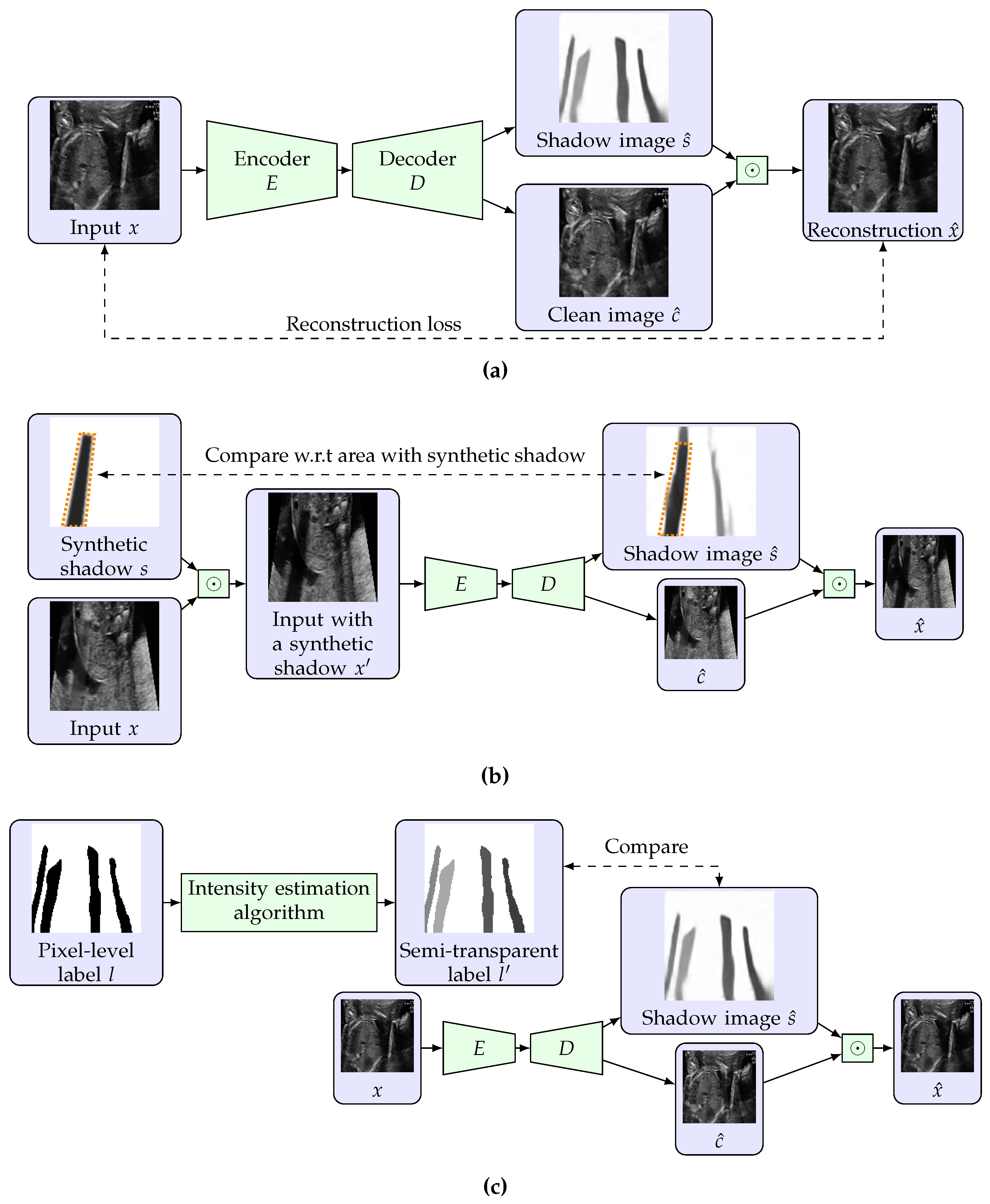
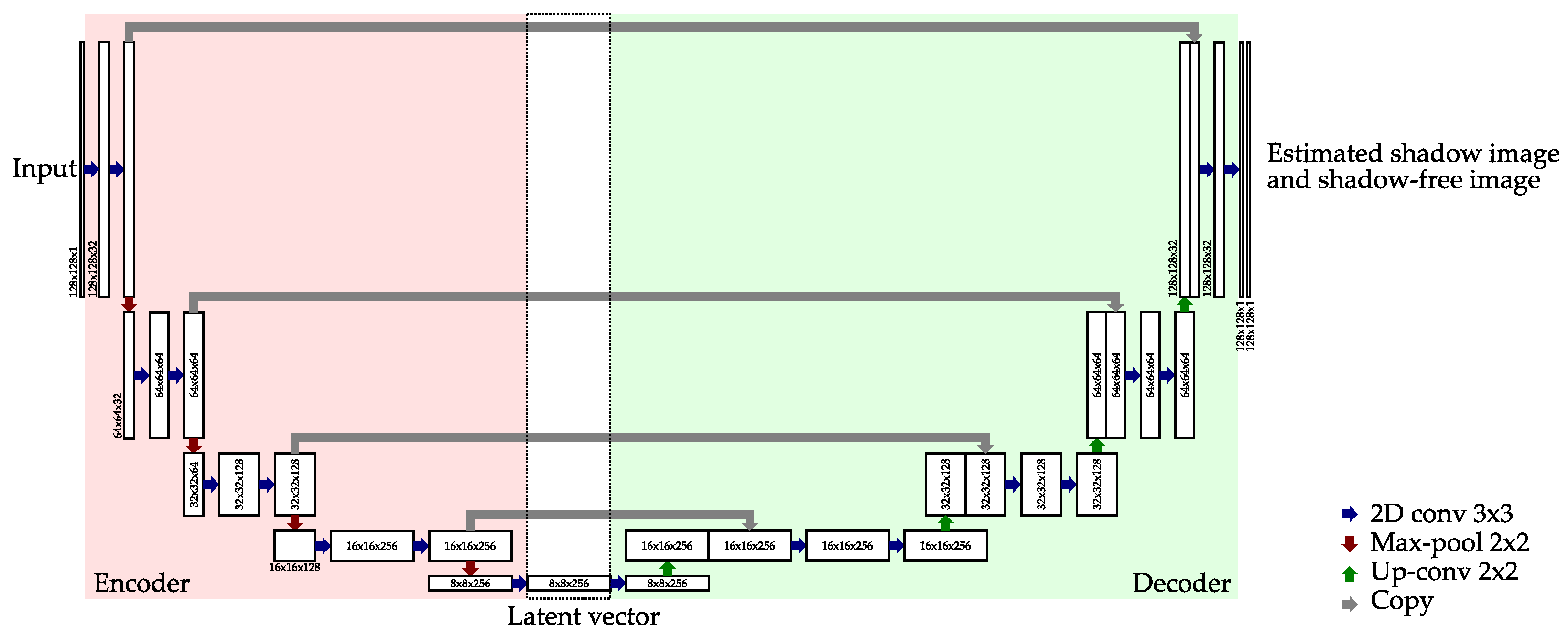
3.2. Restricted Auto-Encoding Structure for Shadow Estimation

Let $x\in {[0,1]}^{H\times W}$ be an input grayscale US image with a size of $H\times W$. Its brightness is assumed to be normalized to $[0,1]$. We introduce an encoder DNN $E:{[0,1]}^{H\times W}\to {\mathbb{R}}^m$ and a decoder DNN $D:{\mathbb{R}}^m\to {[0,1]}^{H\times W\times 2}$, where m is the number of dimensions of a latent vector. Note that the decoder D outputs an image with two channels. An auto-encoding procedure that reconstructs the input x into $\widehat{x}$ is defined as

$$\begin{array}{c}\widehat{x}=\widehat{s}\odot \widehat{c},\end{array}$$

(1)

$$\begin{array}{c}\tilde{x}:=D\left(E\left(x\right)\right),\widehat{s}:={\tilde{x}}_1,\widehat{c}:={\tilde{x}}_2,\end{array}$$

(2)

where $\odot ,{\tilde{x}}_i,\widehat{s}$ and $\widehat{c}$ are element-wise product, the i-th channel of $\tilde{x}$, the estimated shadow image, and the estimated clean image without shadows, respectively. For each element in the estimated shadow $\widehat{s}$, $1.0$ means that no shadows expected in the pixel, and the lower the value, the intensity of the estimated shadow is higher. Figure 1a shows the proposed auto-encoding structure.

The reconstruction $\widehat{x}$ is given as Equation (1) because we assume that the input image with shadows is generated as an element-wise product of an ideal shadow-free input image and an image of semi-transparent shadows. This is different from the actual generation process of US images but we model US images with shadows in this way for simplicity.

3.3. Training Using Unlabeled Data with Synthetic Shadows

Since the proposed model is based on auto-encoders, it is basically trained by minimizing a reconstruction loss given as

$$L_{\mathrm{recon}}(x,\widehat{x}):=\frac{1}{HW}\sum _{h=1}^H\sum _{w=1}^W{({\widehat{x}}_{hw}-x_{hw})}^2,$$

(3)

which is also known as the mean squared error (MSE). Of course, we cannot make the model split the input into the estimated shadow and the estimated clean image only by the reconstruction loss. To address this, we introduce synthetic shadows and a loss function that uses them as pseudo labels.

Annotating shadows is costly because the pixel-level label is expensive in the first place, and additionally, shadows are ambiguous. It is difficult to make a standard for labeling shadows that come in various intensities and are often blurred. However, the possible shapes of shadows are known when the domain is fixed; the target to be diagnosed and equipment such as probes are set. Once the shapes are determined, we can generate random plausible synthetic shadows in a rule-based manner. Then the synthetic shadows can be injected into the input image and can be used as pseudo labels. In this study, we focus on convex probes [1] that generate shadows shaped annular sectors. Details of the algorithm for generating shadows are described in Appendix A.

Assuming that a synthetic shadow image $s\in {[0,1]}^{H\times W}$ is given, we inject it to an input image x as follows;

$$x^{\prime }=x\odot s,$$

(4)

and we use $x^{\prime }$ as a new input to the model. A loss function for training the model to predict shadows is defined as

$$L_{\mathrm{synth}}(s,\widehat{s}):=\frac{1}{HW}\sum _{h=1}^H\sum _{w=1}^W\mathbf{1}[s_{hw}\ne 1]{({\widehat{s}}_{hw}-s_{hw})}^2,$$

(5)

where $\mathbf{1}\left[·\right]$ is a function that returns 1 when the condition is met and returns 0 otherwise. Note that the loss $L_{\mathrm{synth}}$ evaluates the area that the synthetic shadow exists. This is because we do not know whether the original input already contains shadows. If the masking term $\mathbf{1}[s_{hw}\ne 1]$ is omitted, the model learns the region without the synthetic shadow as a shadow-free region regardless of the presence of real shadows. Thanks to the mask, we can train the model to estimate the intensity of the synthetic shadow, but the whole estimated shadow tends to be dark. To prevent the estimated shadow $\widehat{s}$ from being too dark and to make the default output white, we also introduce an auxiliary regularization loss defined as

$$L_{\mathrm{synthreg}}\left(\widehat{s}\right):=\frac{1}{HW}\sum _{h=1}^H\sum _{w=1}^W|{\widehat{s}}_{hw}-1|.$$

(6)

A linear combination of the three losses introduced above is a loss for training with unlabeled US images. That is, the loss function is given as

$$L_{\mathrm{unlabeled}}(x,s,\widehat{x},\widehat{s}):={\lambda }_{\mathrm{recon}}{L}_{\mathrm{recon}}(x,\widehat{x})+{\lambda }_{\mathrm{synth}}{L}_{\mathrm{synth}}(s,\widehat{s})+{\lambda }_{\mathrm{synthreg}}{L}_{\mathrm{synthreg}}\left(\widehat{s}\right),$$

(7)

where ${\lambda }_{\mathrm{recon}},{\lambda }_{\mathrm{synth}},{\lambda }_{\mathrm{synthreg}}>0$ are hyperparameters that decide the weight of each loss. This training procedure using unlabeled data and the synthetic shadows is illustrated in Figure 1b.

3.4. Use of Pixel-Level Labels and Extension to Semi-Supervised Learning

Pixel-level labels for US shadows are expensive as mentioned above, but if available, they can contribute to the improvement of the estimation performance. We assume that we have some pixel-level labeled data which labels are binary; whether each pixel is in shadows or not. Ideally, we expect labels that express semi-transparency of shadows but the correct intensities of shadows are unknown even for experts. Hence, we introduce a method to effectively utilize the binary labels for the proposed shadow estimation framework.

Let $l\in {\{0,1\}}^{H\times W}$ be a pixel-level binary label that represents where shadows exist. For each element in l, 0 and 1 correspond to a shadowed pixel and a shadow-free pixel, respectively. Recall that the proposed auto-encoding model is based on the idea: each input US image is considered to be generated by an element-wise product of the ideal shadow-free image and the shadow image. If the ideal shadow-free image $x^{*}$ for an input x is available, we can calculate the intensity of the labeled shadow by

$$l_{hw}^{*}:=\left\{\begin{array}{cc}{\displaystyle \frac{x_{hw}}{x_{hw}^{*}}}\hfill & (l_{hw}=0)\hfill \\ {\displaystyle 1}\hfill & (l_{hw}=1)\hfill \end{array}\right..$$

(8)

However, $x^{*}$ is actually unknown. Here, we estimate $x^{*}$ as a mean brightness over the shadow-free area that is written as

$${\widehat{x}}^{*}:=\frac{1}{{\sum }_{i,j}{M}_{ij}}\sum _{i=1}^H\sum _{j=1}^W{M}_{ij}{x}_{ij},$$

(9)

where $M\in {\{0,1\}}^{H\times W}$ is a mask that represents the region without shadows. The mask M is given as

$$M_{hw}:=\left\{\begin{array}{cc}{\displaystyle 1}\hfill & (l_{hw}=1\mathrm{and}{x}_{hw}>T)\hfill \\ {\displaystyle 0}\hfill & \left(\mathrm{otherwise}\right)\hfill \end{array}\right.,$$

(10)

where $T\in [0,1]$ is a given threshold to ignore almost completely black areas that have no shadows. In US images, liquids are shown in black. By thresholding, we can reject such areas and estimate $x^{*}$ more precisely. Besides, for simplicity and stability of the training, we assume that the intensity of each labeled shadow is constant. Hence, Equation (8) is rewritten and the resulting label with the estimated intensity is

$$l_{hw}^{\prime }:=\left\{\begin{array}{cc}{\displaystyle \frac{1}{{\widehat{x}}^{*}}·\frac{{\sum }_{z\in \mathcal{S}\left(x_{hw}\right)}z}{\left|\mathcal{S}\right(x_{hw}\left)\right|}}\hfill & (l_{hw}=0)\hfill \\ {\displaystyle 1}\hfill & (l_{hw}=1)\hfill \end{array}\right.,$$

(11)

where $\mathcal{S}\left(x_{hw}\right)$ is a subset of $\left\{x_{ij}\right\}(i=1,\cdots ,H,j=1,\cdots ,W)$ that consists of $x_{ij}$ inside the shadow that contains $x_{ij}$. Calculation of $l^{\prime }$ is summarized in Algorithm 1.

Algorithm 1 Estimation of shadow intensities using a pixel-level binary label.

Input: A US image $x\in {[0,1]}^{H\times W}$, a pixel-level label of shadows $l\in {\{0,1\}}^{H\times W}$, and a threshold T.

Output: Semi-transparent label $l^{\prime }\in {[0,1]}^{H\times W}$

1: $M\leftarrow l\odot \mathbf{1}[x>T]$

2: $x^{*}\leftarrow \frac{1}{{\sum }_{i,j}{M}_{ij}}{\sum }_{i=1}^H{\sum }_{j=1}^W{M}_{ij}{x}_{ij}$

3: $l^{\prime }\leftarrow l$

4: for each labeled shadow $l_c$ in l (i.e., each connected component $l_c$ in l with a value 0) do

5:  for each coordinate $(i,j)$ that corresponds to $l_c$ do

6:   $l_{ij}^{\prime }\leftarrow l_{ij}^{\prime }+\frac{x_{ij}}{{\widehat{x}}^{*}\left|l_c\right|}$

7:  end for

8: end for

Using the estimated semi-transparent label $l^{\prime }$, we can construct a loss function based on Equation (5) as follows;

$$L_{\mathrm{label}}(l^{\prime },\widehat{s}):=\frac{1}{HW}\sum _{h=1}^H\sum _{w=1}^W{({\widehat{s}}_{hw}-l_{hw}^{\prime })}^2.$$

(12)

In contrast to Equation (5), we do not need the masking term anymore because the label $l^{\prime }$ tells not only shadowed areas but also shadow-free areas. Besides, the regularization term given by Equation (6) is neither needed. The resulting loss function for labeled data is given as

$$L_{\mathrm{labeled}}(x,l^{\prime },\widehat{x},\widehat{s}):={\lambda }_{\mathrm{recon}}{L}_{\mathrm{recon}}(x,\widehat{x})+{\lambda }_{\mathrm{label}}{L}_{\mathrm{label}}(l^{\prime },\widehat{s}),$$

(13)

where ${\lambda }_{\mathrm{recon}},{\lambda }_{\mathrm{label}}>0$ are hyperparameters. Figure 1c illustrates the training procedure with labeled data.

By switching Equations (7) and (13) according to the existence of labels, we can train the proposed model in a semi-supervised fashion that effectively utilizes both unlabeled data and labeled data. Assume that an unlabeled dataset ${\mathcal{D}}_{\mathrm{unlabeled}}=\{x^1,\cdots ,x^{N_{\mathrm{unlabeled}}}\}$ and a labeled dataset ${\mathcal{D}}_{\mathrm{labeled}}=\{(x^1,l^1),\cdots ,(x^{N_{\mathrm{labeled}}},l^{N_{\mathrm{labeled}}})\}$ are given, where $N_{\mathrm{unlabeled}}$ and $N_{\mathrm{labeled}}$ are the number of unlabeled data and that of labeled data, respectively. Then, a mini-batch $\mathcal{B}\subset {\mathcal{D}}_{\mathrm{unlabeled}}\cup {\mathcal{D}}_{\mathrm{labeled}}$ can be drawn. The loss for the mini-batch is given as

$$L\left(\mathcal{B}\right)=\frac{1}{\left|\mathcal{B}\right|}\left[\sum _{{x\in \mathcal{B}|}_{\mathrm{unlabeled}}}{L}_{\mathrm{unlabeled}}(x,s,\widehat{x},\widehat{s})+\sum _{{(x,l)\in \mathcal{B}|}_{\mathrm{labeled}}}{L}_{\mathrm{labeled}}(x,l^{\prime },\widehat{x},\widehat{s})\right].$$

(14)

Note that s and $l^{\prime }$ should be generated for each sample in the batch.

4. Results

4.1. Setting

The encoder E and the decoder D were constructed just like U-Net [30]. Details of the architecture are described in Appendix B. The model was optimized by Adam [34]. The size of the mini-batch was 32 and the number of training epochs was 10. The parameters of Adam were set to default except for the learning rate $\alpha$ that was set ${10}^{-4}$ initially and decayed to ${10}^{-5}$ through 10 epochs of training. The weight for the reconstruction error ${\lambda }_{\mathrm{recon}}$ was fixed to $1.0$. Other hyperparameters were set by grid search using the validation data. The search spaces of the hyperparameters are following: ${\lambda }_{\mathrm{synth}}={\lambda }_{\mathrm{label}}\in \{{10}^{-2},{10}^{-1},1,10,{10}^2,{10}^3\}$, ${\lambda }_{\mathrm{synthreg}}\in \{{10}^{-3},{10}^{-2},{10}^{-1},1,10\}$, and $v_{\min }\in \{0.1,0.5\}$ in Algorithm A1. Note that ${\lambda }_{\mathrm{synthreg}}$ was set to zero in the semi-supervised situations because we empirically found that the labels play the same role as the regularization term. The selected hyperparameters are shown in Appendix C. To stabilize the training, in semi-supervised situations, the labeled training dataset was oversampled so that the number of the labeled data was almost equal to the size of the unlabeled dataset. Specifically, the labeled data was simply repeated $\lfloor N_{\mathrm{unlabeled}}/N_{\mathrm{labeled}}\rfloor$ times.

As a reference DNN based segmentation method, we used vanilla U-Net [30]. It was trained on pixel-wise cross-entropy and optimized by Adam with $\alpha ={10}^{-4}$. The size of the mini-batch was 32. Because U-Net only uses the labeled dataset, the number of training epochs was set so that the number of iterations equals that of the proposed method to prevent underfitting. We empirically confirmed that the training of U-Net converged with this setting.

For both the proposed method and U-Net, the parameters of the models were saved every epoch. Then, the parameters that perform best for the validation dataset were selected. In addition, random cropping is applied to input data and they are resized to $128\times 128$ for both the methods.

The geometrical method [19] and the random walk method [20] are also used as references of methods that do not use labels. The parameters were in accordance with the original papers. Because the geometrical method outputs shadow detection results along scattered scanlines, we applied morphological closing filters to the results for adjusting to pixel-level detection.

We show the experimental results on the testing dataset in the following sections. For all the experiments, the testing images are cropped so that they contain no meta-data and resized to $128\times 128$. Quantitative results for the validation dataset is shown in Appendix D.

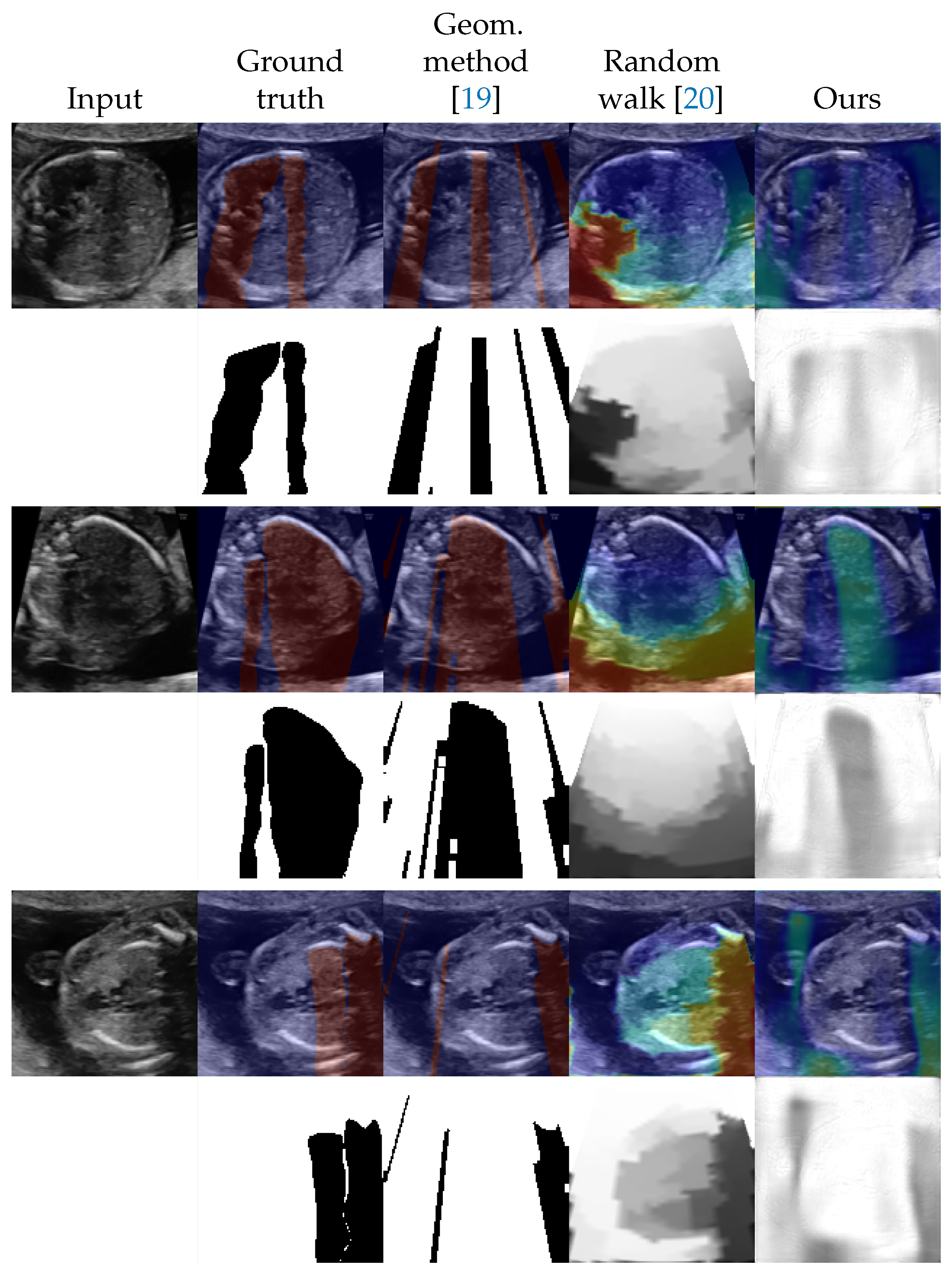
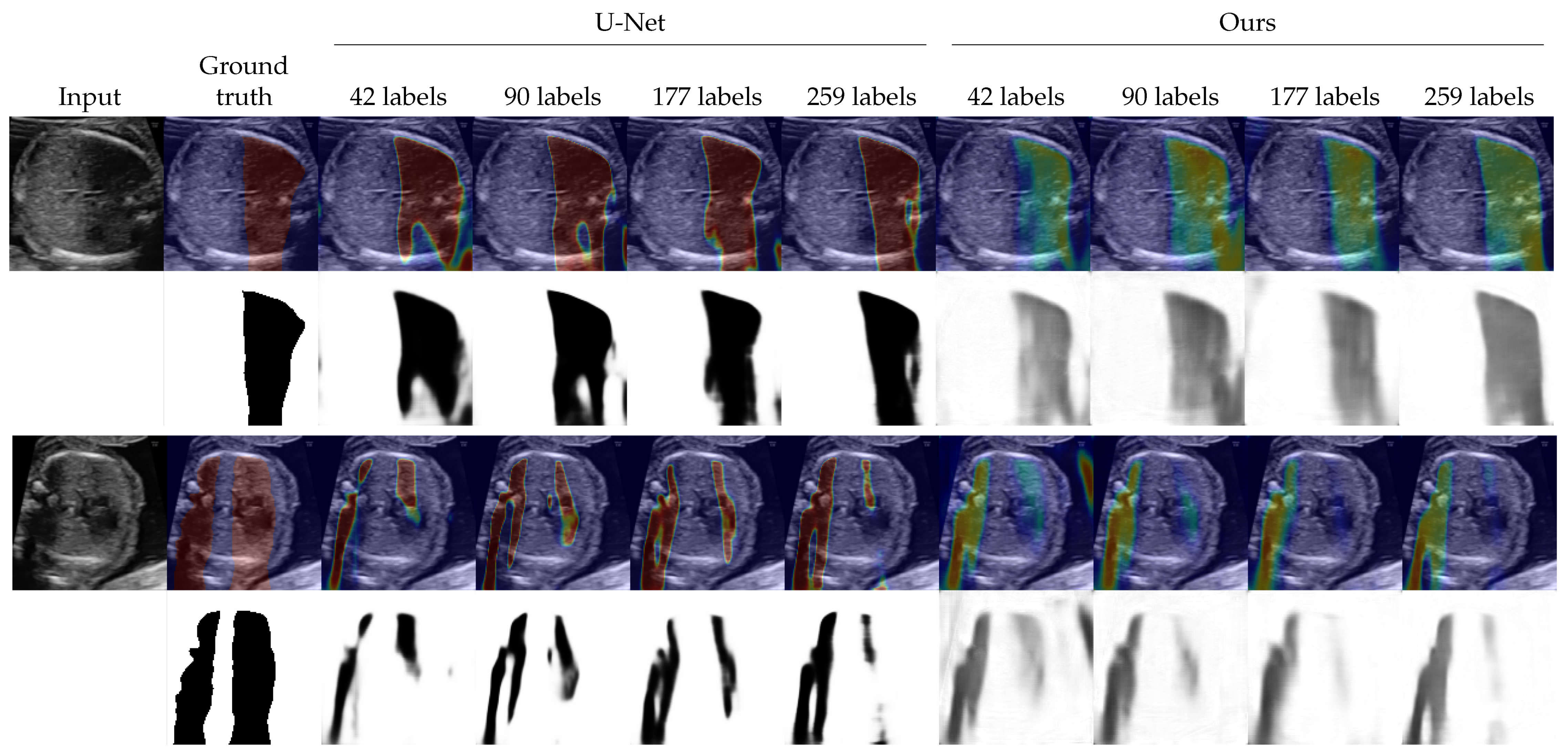
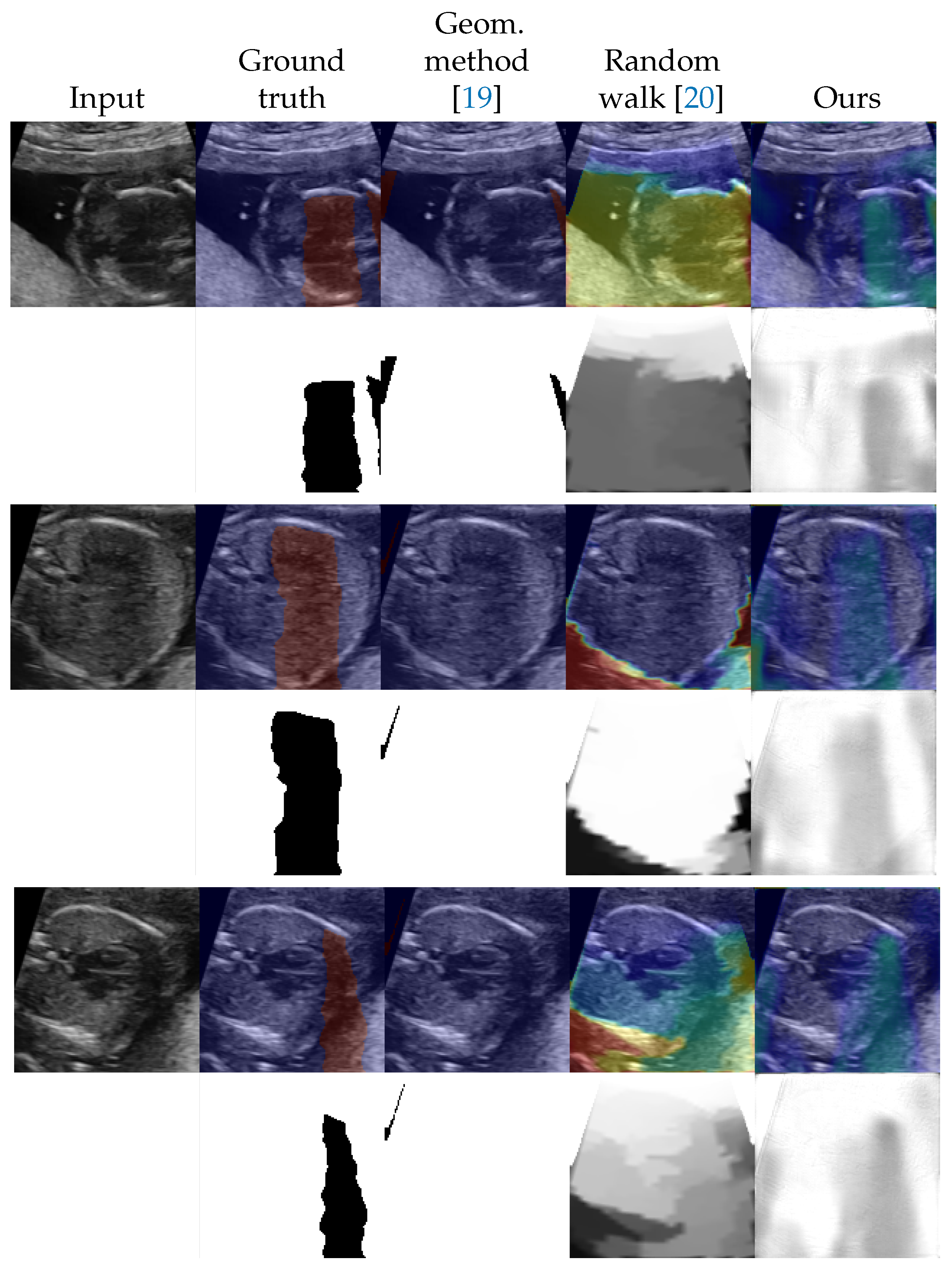
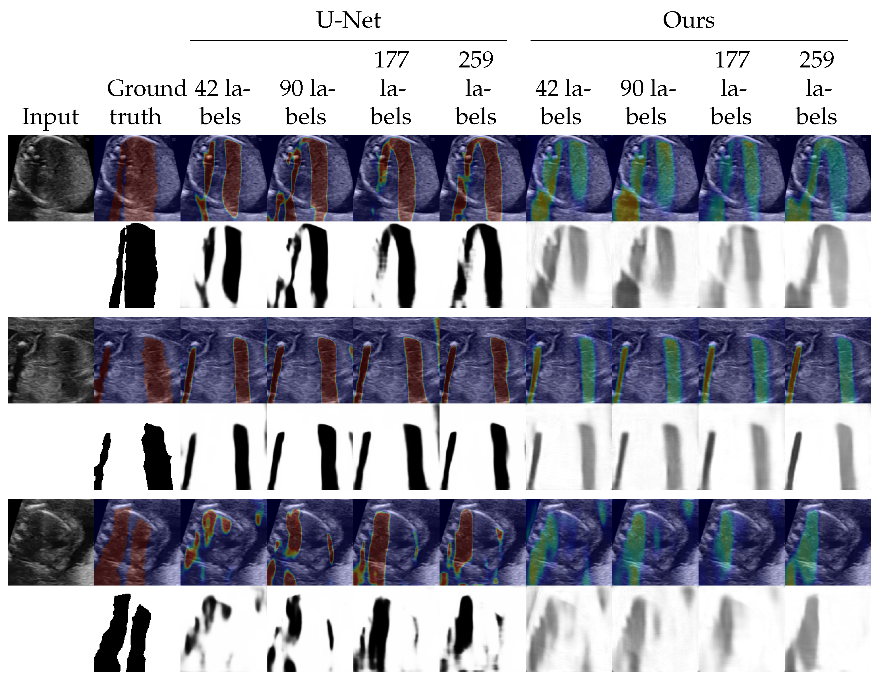
4.2. Shadow Detection

We evaluated the proposed method as a shadow detection method. In situations with labels, we investigated the performance on different numbers of labeled data. The numbers of labeled training data were set to 0, 42 (from 5 videos), 90 (from 10 videos), 177 (from 20 videos), and 259 (from all 30 videos). Since the proposed method estimates intensities of shadows as $\widehat{s}$, a threshold to convert $\widehat{s}$ to binary was searched using the validation dataset. The threshold is selected from $\{0.001,0.002,\cdots ,0.999\}$. For the random walk method [20] which estimates confidence maps, we also searched and applied a threshold in the same way as the proposed method. The selected thresholds are shown in Appendix C. The detection performance was evaluated by the DICE score [35] which is also known as F1 measure.

Table 1. Results of shadow detection evaluated in the DICE score. The scores are calculated for each testing image, and means over them are shown. The numbers in parentheses are the standard deviations.

	Number of Labeled Images
Method	0	42 (5 Videos)	90 (10 Videos)	177 (20 Videos)	259 (30 Videos)
Geometric method [19]	0.193 (±0.210)	-	-	-	-
Random walk [20]	0.450 (±0.142)	-	-	-	-
U-Net [30]	-	0.610 (±0.184)	0.655 (±0.170)	0.681 (±0.136)	0.698 (±0.137)
Ours	0.578 (±0.164)	0.666 (±0.142)	0.686 (±0.148)	0.707 (±0.113)	0.720 (±0.151)

shows the results in the DICE score. Figure 2 and Figure 3 shows examples of shadow detection of the methods that do not use labels and the methods that use labels, respectively (for additional results, see Figure A2 and Figure A3).

In the unlabeled situation, we can see that the proposed method outperformed the other two methods from Table 1. The standard deviation was large for the geometric method. The score of the geometric method is low but Figure 2 shows that performed well in some examples. The random walk method scored better than that of the geometric method and detected shadows that the geometric method could not. However, the outputs of the random walk method tended to simply reflect the distance from the probe. The proposed method estimated the shapes of the shadows well although the estimation results tend to be blurred. Figure 2 also indicates that the proposed method successfully estimated the intensities of the shadows.

In terms of the methods that use labeled data, that is, U-Net and the proposed method in semi-supervised situations, the proposed method performed slightly better than U-Net as Table 1 shows. We could see no clear trends for the standard deviations. The differences in the DICE score were larger when the numbers of labeled data were smaller. Figure 3 shows that the two methods detected shadows in almost the same performance. The proposed method expressed the intensities of the shadows while U-Net output the detection result in maps that are almost binary.

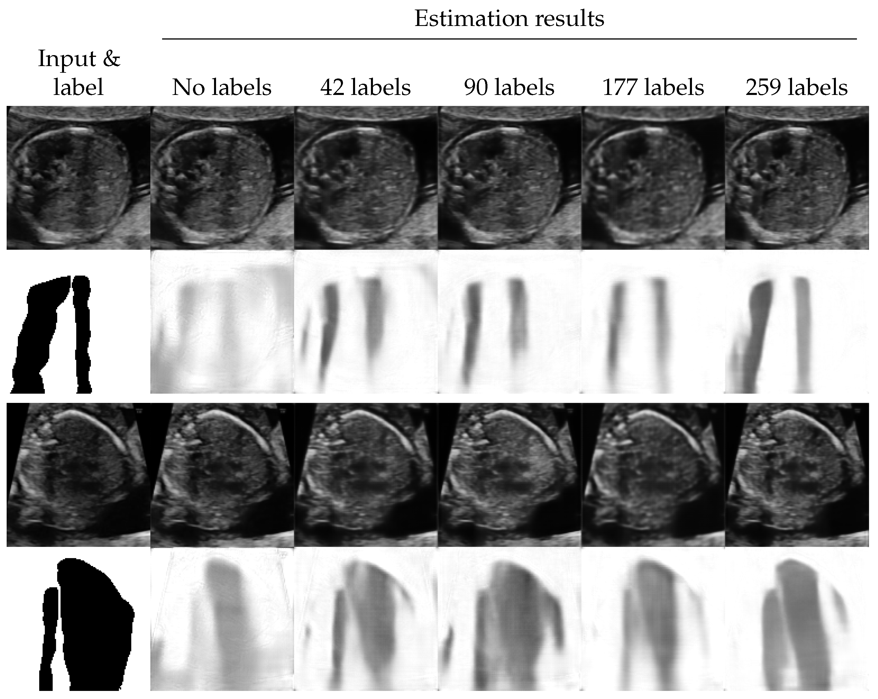
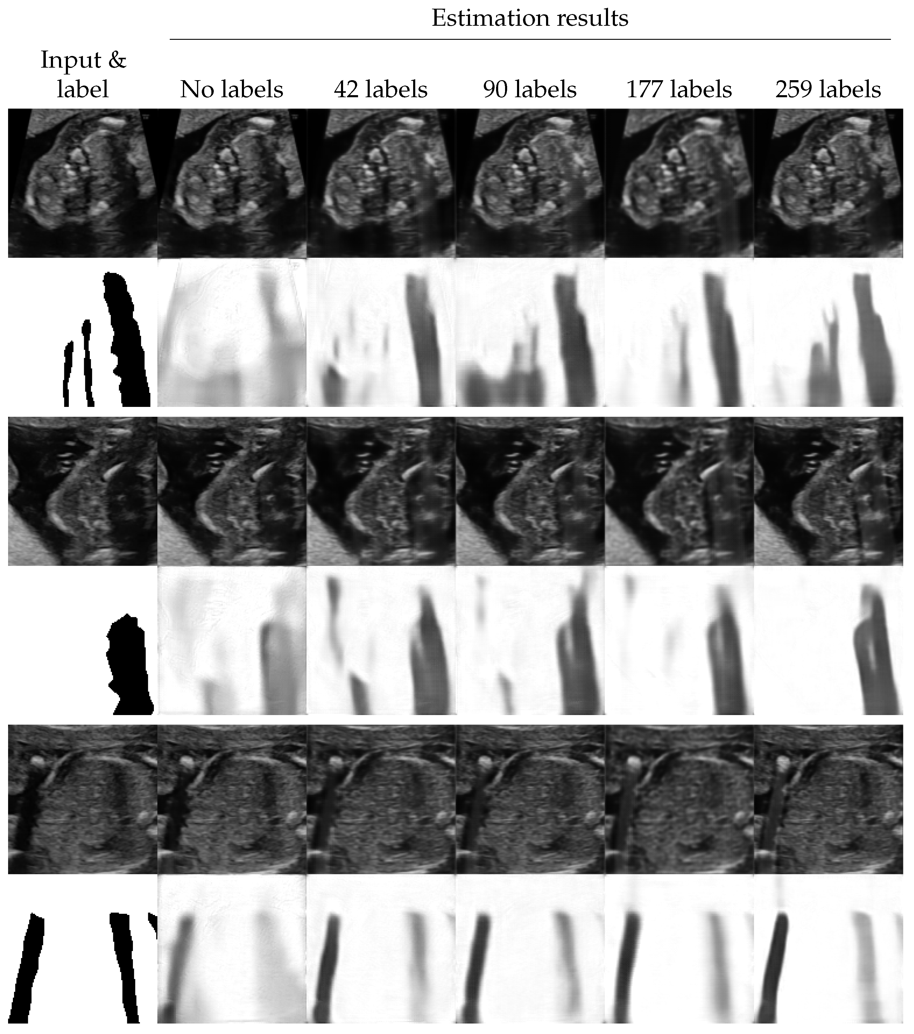
4.3. Shadow Intensity Estimation

We evaluated the performance of the proposed method in the estimation of intensities of shadows. Since we do not have the ground truth for shadow intensities, as a novel indicator, we calculated the correlations of the brightness of the input image and the estimation with respect to the area labeled as shadows. More specifically, given an input image x, a pixel-label l, and a shadow estimation $\widehat{s}$, the indicator is calculated as follows;

$$\begin{array}{c}\rho (x,l,\widehat{s}):=\frac{{\sum }_{h=1}^H{\sum }_{w=1}^W(1-l_{hw})(x_{hw}-\overline{x})({\widehat{s}}_{hw}-\overline{s})}{\sqrt{{\sum }_{h=1}^H{\sum }_{w=1}^W(1-l_{hw}){(x_{hw}-\overline{x})}^2}\sqrt{{\sum }_{h=1}^H{\sum }_{w=1}^W(1-l_{hw}){({\widehat{s}}_{hw}-\overline{s})}^2}},\end{array}$$

(15)

$$\begin{array}{c}\overline{x}=\frac{{\sum }_{h=1}^H{\sum }_{w=1}^W(1-l_{hw})x_{hw}}{{\sum }_{h=1}^H{\sum }_{w=1}^W(1-l_{hw})},\overline{s}=\frac{{\sum }_{h=1}^H{\sum }_{w=1}^W(1-l_{hw}){\widehat{s}}_{hw}}{{\sum }_{h=1}^H{\sum }_{w=1}^W(1-l_{hw})},\end{array}$$

(16)

which is Pearson’s correlation coefficient [36] that is masked using the label l.

Table 2. Evaluation of the estimation of shadow intensities. Scores are the correlation coefficient calculated by Equation (15). The coefficients are calculated for each testing image, and means over them are shown. The numbers in parentheses are the standard deviations.

	Number of Labeled Images
Method	0	42 (5 Videos)	90 (10 Videos)	177 (20 Videos)	259 (30 Videos)
Geometric method [19]	0.152 (±0.182)	-	-	-	-
Random walk [20]	−0.047 (±0.290)	-	-	-	-
U-Net [30]	-	0.308 (±0.150)	0.267 (±0.144)	0.262 (±0.158)	0.247 (±0.172)
Ours	0.351 (±0.155)	0.388 (±0.150)	0.414 (±0.159)	0.358 (±0.149)	0.349 (±0.162)

shows the results. Since the conventional methods are designed for detecting shadows and not estimating their intensities, the coefficients for them were just for benchmarks. It illustrates that the proposed method achieved the largest coefficients for all the numbers of labeled data. This indicates that our method estimated the shadow intensities the most precisely among the methods we examined. The coefficients of U-Net are lower than that of the proposed method but it was stable. The methods based on image processing, the geometric method and the random walk, performed worse. Especially, the estimation of the random walk method is the worst and had almost no correlations to the input image, despite its better performance for shadow detection than the geometric method. The standard deviation of the random walk method was larger than other methods and the method seemed to be unstable for this indicator.

4.4. Shadow Removal

The proposed method estimated shadows and shadow-free variants of the input images at the same time. We evaluated the quality of the estimated shadow-free images subjectively.

Figure 4 shows the examples of shadow removal performed by the proposed method (for additional results, see Figure A4). We observed that the areas with low-intensity shadows were efficiently enhanced. Additionally, the quality of the enhancement seemed better when the performance of shadow detection was better. In contrast, the shadows with high intensities tended to be just filled with blurred texture.

5. Discussion

Among the shadow detecting methods which do not use labels, the proposed method detected shadows the most correctly. The other two methods could suffer from the difference of domains; the domains for which the methods were built and the domain of fetal heart diagnosis that we used in this paper. Besides, the standard deviation of the DICE score for the geometric method was large. This means that its detection performance varies among the testing images. This is probably because the method heavily depends on the domain for which it is designed. In that sense, our method has an advantage because it is data-driven. Although the proposed method also uses domain-specific knowledge, it only requires rough possible shapes of shadows that are determined mainly by the type of the probe. In the situations that the labels are available, the proposed method achieved comparable detection performance to U-Net which is a popular segmentation method for medical images. When only 42 labeled images were used for training, our method was better than U-Net. The auto-encoding structure possibly helped detection by extracting features by the unlabeled data. The maximum number of labeled data, 259 from 30 videos, was relatively small in the context of DNNs, but both the proposed method and U-Net performed well. In terms of detecting shadows, the dataset was clean and in a narrow domain, and it might be easy to detect shadows. From the perspective of data collection, we revealed that a couple of hundred of labeled data is enough for one domain. The amount is reasonable when it comes to accumulating data of different multiple domains.

One of the advantages of the proposed method is that it can estimate the intensities of shadows. Although we cannot obtain the ground truth of the intensities, our method estimated images of shadows which intensities are highly correlated to the brightness of the shadowed areas of the input images, at least. The correlation coefficients were higher than the other methods we used in the experiments. From the intensities of shadows, we can assess the quality of US images using them. If we detect shadows in a binary segmentation manner, the sizes of shadowed areas can be used for quality inspection. Our method can provide additional information, the intensities of shadows, and we can check US images based on it; an US image with large but light shadows should be allowed in some situations, for example.

Although removing shadows is not the main target of our work, notably, our method removed shadows of input US images without training on losses that directly lead the decoder to output clean image as $\widehat{c}$. This result could come from the model structure that split the input into the estimated shadow and the estimated clean input and then compose them into the reconstruction. Besides, the estimated clean images were clear, thanks to the U-Net like structure that has skip-connections between the encoder and the decoder [37]. In a clinical sense, we cannot totally trust the estimated shadow-free images because the shadowed areas are completed statistically. It means that the images of popular and healthy cases are likely to appear even if the target of diagnosis has anomalies. However, generating shadow-free images can work as a pre-processing for image recognition techniques.

6. Conclusions

We proposed an auto-encoding structure-based DNN that estimates acoustic shadows in US images. The method estimates not only the location of shadows but also their intensities. We also introduced the loss functions for training the model on both unlabeled data and labeled data. For unlabeled data, synthetic shadows are generated using the knowledge that the probes decide the shapes of shadows, and used as pseudo labels. If binary pixel-level labels that tell us areas with shadows are given, they are effectively utilized by converting them to labels with estimated intensities. By experiments on US images for fetal heart diagnosis, we showed that our method detected shadows better than the conventional methods in the situation without labels and did better to the DNN-based segmentation method U-Net in the situations with labels available. In terms of estimating the intensities of shadows, the proposed method performed the best. Moreover, we suggested the capability of our method in removing shadows as supplemental outputs, not just estimating them.

Although our method employs the auto-encoding structure that extracts features from input images, the difference in detection performance between fully-supervised U-Net and semi-supervised our method was small. One possible reason for this result is that the detection was easy; the images in the dataset were relatively clear and belonged to the narrow domain. Applying to datasets that are in different domains or have more variations of images has remained as one of the future work.

The proposed method can work with any US image recognition methods as a pre-processing. We can reject low-quality data based on the estimated shadow images. The use in such quality assessing ways is one of the possible future directions.

References

1. Szabo, T.L. Diagnostic Ultrasound Imaging: Inside Out; Academic Press: Cambridge, MA, USA, 2004. [Google Scholar]
2. Moran, C.M.; Pye, S.D.; Ellis, W.; Janeczko, A.; Morris, K.D.; McNeilly, A.S.; Fraser, H.M. A Comparison of the Imaging Performance of High Resolution Ultrasound Scanners for Preclinical Imaging. Ultrasound Med. Biol. 2011, 37, 493–501. [Google Scholar] [CrossRef] [Green Version]
3. Sassaroli, E.; Crake, C.; Scorza, A.; Kim, D.S.; Park, M.A. Image Quality Evaluation of Ultrasound Imaging Systems: Advanced B-Modes. J. Appl. Clin. Med. Phys. 2019, 20, 115–124. [Google Scholar] [CrossRef]
4. Entrekin, R.R.; Porter, B.A.; Sillesen, H.H.; Wong, A.D.; Cooperberg, P.L.; Fix, C.H. Real-Time Spatial Compound Imaging: Application to Breast, Vascular, and Musculoskeletal Ultrasound. Semin. Ultrasound CT MRI 2001, 22, 50–64. [Google Scholar] [CrossRef]
5. Desser, T.S.; Jeffrey, R.B., Jr.; Lane, M.J.; Ralls, P.W. Tissue Harmonic Imaging: Utility in Abdominal and Pelvic Sonography. J. Clin. Ultrasound 1999, 27, 135–142. [Google Scholar] [CrossRef]
6. Ortiz, S.H.C.; Chiu, T.; Fox, M.D. Ultrasound Image Enhancement: A Review. Biomed. Signal Process. Control 2012, 7, 419–428. [Google Scholar] [CrossRef]
7. Perdios, D.; Vonlanthen, M.; Besson, A.; Martinez, F.; Arditi, M.; Thiran, J. Deep Convolutional Neural Network for Ultrasound Image Enhancement. In Proceedings of the 2018 IEEE International Ultrasonics Symposium, Kobe, Japan, 22–25 October 2018. [Google Scholar]
8. Feldman, M.K.; Katyal, S.; Blackwood, M.S. US Artifacts. RadioGraphics 2009, 29, 1179–1189. [Google Scholar] [CrossRef] [PubMed]
9. Ziskin, M.C.; Thickman, D.I.; Goldenberg, N.J.; Lapayowker, M.S.; Becker, J.M. The Comet Tail Artifact. J. Ultrasound Med. 1982, 1, 1–7. [Google Scholar] [CrossRef]
10. Noble, J.A.; Boukerroui, D. Ultrasound Image Segmentation: A Survey. IEEE Trans. Med. Imaging 2006, 25, 987–1010. [Google Scholar] [CrossRef] [Green Version]
11. Brattain, L.J.; Telfer, B.A.; Dhyani, M.; Grajo, J.R.; Samir, A.E. Machine Learning for Medical Ultrasound: Status, Methods, and Future Opportunities. Abdom. Radiol. 2018, 43, 786–799. [Google Scholar] [CrossRef]
12. Liu, S.; Wang, Y.; Yang, X.; Lei, B.; Liu, L.; Li, S.X.; Ni, D.; Wang, T. Deep Learning in Medical Ultrasound Analysis: A Review. Engineering 2019, 5, 261–275. [Google Scholar] [CrossRef]
13. Drukker, L.; Noble, J.A.; Papageorghiou, A.T. Introduction to Artificial Intelligence in Ultrasound Imaging in Obstetrics and Gynecology. Ultrasound Obstet. Gynecol. 2020, 56, 498–505. [Google Scholar] [CrossRef] [PubMed]
14. Dozen, A.; Komatsu, M.; Sakai, A.; Komatsu, R.; Shozu, K.; Machino, H.; Yasutomi, S.; Arakaki, T.; Asada, K.; Kaneko, S.; et al. Image Segmentation of the Ventricular Septum in Fetal Cardiac Ultrasound Videos Based on Deep Learning Using Time-Series Information. Biomolecules 2020, 10, 1526. [Google Scholar] [CrossRef] [PubMed]
15. Shozu, K.; Komatsu, M.; Sakai, A.; Komatsu, R.; Dozen, A.; Machino, H.; Yasutomi, S.; Arakaki, T.; Asada, K.; Kaneko, S.; et al. Model-Agnostic Method for Thoracic Wall Segmentation in Fetal Ultrasound Videos. Biomolecules 2020, 10, 1691. [Google Scholar] [CrossRef] [PubMed]
16. LeCun, Y.; Bengio, Y.; Hinton, G. Deep Learning. Nature 2015, 521, 436–444. [Google Scholar] [CrossRef] [PubMed]
17. Komatsu, M.; Sakai, A.; Komatsu, R.; Matsuoka, R.; Yasutomi, S.; Shozu, K.; Dozen, A.; Machino, H.; Hidaka, H.; Arakaki, T.; et al. Detection of Cardiac Structural Abnormalities in Fetal Ultrasound Videos Using Deep Learning. Appl. Sci. 2021, 11, 371. [Google Scholar] [CrossRef]
18. Vincent, P.; Larochelle, H.; Lajoie, I.; Bengio, Y.; Manzagol, P.A. Stacked Denoising Autoencoders: Learning Useful Representations in a Deep Network with a Local Denoising Criterion. J. Mach. Learn. Res. 2010, 11, 3371–3408. [Google Scholar]
19. Hellier, P.; Coupé, P.; Morandi, X.; Collins, D.L. An Automatic Geometrical and Statistical Method to Detect Acoustic Shadows in Intraoperative Ultrasound Brain Images. Med. Image Anal. 2010, 14, 195–204. [Google Scholar] [CrossRef] [Green Version]
20. Karamalis, A.; Wein, W.; Klein, T.; Navab, N. Ultrasound Confidence Maps Using Random Walks. Med. Image Anal. 2012, 16, 1101–1112. [Google Scholar] [CrossRef]
21. Hacihaliloglu, I. Enhancement of bone shadow region using local phase-based ultrasound transmission maps. Int. J. Comput. Assist. Radiol. Surg. 2017, 12, 951–960. [Google Scholar] [CrossRef]
22. Meng, Q.; Baumgartner, C.; Sinclair, M.; Housden, J.; Rajchl, M.; Gomez, A.; Hou, B.; Toussaint, N.; Zimmer, V.; Tan, J.; et al. Automatic Shadow Detection in 2D Ultrasound Images. In Data Driven Treatment Response Assessment and Preterm, Perinatal, and Paediatric Image Analysis, Granada, Spain, 16 September 2018; Springer: Berlin/Heidelberg, Germany, 2018; pp. 66–75. [Google Scholar]
23. Meng, Q.; Sinclair, M.; Zimmer, V.; Hou, B.; Rajchl, M.; Toussaint, N.; Oktay, O.; Schlemper, J.; Gomez, A.; Housden, J.; et al. Weakly Supervised Estimation of Shadow Confidence Maps in Fetal Ultrasound Imaging. IEEE Trans. Med. Imaging 2019, 38, 2755–2767. [Google Scholar] [CrossRef]
24. Hu, R.; Singla, R.; Yan, R.; Mayer, C.; Rohling, R.N. Automated Placenta Segmentation with a Convolutional Neural Network Weighted by Acoustic Shadow Detection. In Proceedings of the 2019 41st Annual International Conference of the IEEE Engineering in Medicine and Biology Society, Berlin, Germany, 23–27 July 2019; pp. 6718–6723. [Google Scholar]
25. Goodfellow, I.; Bengio, Y.; Courville, A.; Bengio, Y. Deep Learning; MIT Press: Cambridge, MA, USA, 2016. [Google Scholar]
26. Kingma, D.P.; Welling, M. Auto-Encoding Variational Bayes. arXiv 2014, arXiv:1312.6114. [Google Scholar]
27. Makhzani, A.; Shlens, J.; Jaitly, N.; Goodfellow, I.; Frey, B. Adversarial Autoencoders. arXiv 2016, arXiv:1511.05644. [Google Scholar]
28. Rasmus, A.; Berglund, M.; Honkala, M.; Valpola, H.; Raiko, T. Semi-Supervised Learning with Ladder Networks. In Advances in Neural Information Processing Systems, Montréal, Canada, 7–10 December 2015; Curran Associates, Inc.: Red Hook, NY, USA, 2015; Volume 28, pp. 3546–3554. [Google Scholar]
29. Garcia-Garcia, A.; Orts-Escolano, S.; Oprea, S.; Villena-Martinez, V.; Martinez-Gonzalez, P.; Garcia-Rodriguez, J. A Survey on Deep Learning Techniques for Image and Video Semantic Segmentation. Appl. Soft Comput. 2018, 70, 41–65. [Google Scholar] [CrossRef]
30. Ronneberger, O.; Fischer, P.; Brox, T. U-Net: Convolutional Networks for Biomedical Image Segmentation. In International Conference on Medical Image Computing and Computer-Assisted Intervention, Proceedings of the MICCAI 2015: Medical Image Computing and Computer-Assisted Intervention, Munich, Germany, 5–9 October 2015; Springer: Berlin/Heidelberg, Germany, 2015; pp. 234–241. [Google Scholar]
31. Chen, C.; Qin, C.; Qiu, H.; Tarroni, G.; Duan, J.; Bai, W.; Rueckert, D. Deep Learning for Cardiac Image Segmentation: A Review. Front. Cardiovasc. Med. 2020, 7, 25. [Google Scholar] [CrossRef] [PubMed]
32. Wang, L.W.; Siu, W.C.; Liu, Z.S.; Li, C.T.; Lun, D.P.K. Deep Relighting Networks for Image Light Source Manipulation. In Proceedings of the the 2020 European Conference on Computer Vision, Glasgow, UK, 23–28 August 2020. [Google Scholar]
33. Yasutomi, S.; Arakaki, T.; Hamamoto, R. Shadow Detection for Ultrasound Images Using Unlabeled Data and Synthetic Shadows. arXiv 2019, arXiv:1908.01439. [Google Scholar]
34. Kingma, D.P.; Ba, J. Adam: A Method for Stochastic Optimization. In Proceedings of the 3rd International Conference on Learning Representations, San Diego, CA, USA, 7–9 May 2015. [Google Scholar]
35. Carass, A.; Roy, S.; Gherman, A.; Reinhold, J.C.; Jesson, A.; Arbel, T.; Maier, O.; Handels, H.; Ghafoorian, M.; Platel, B.; et al. Evaluating White Matter Lesion Segmentations with Refined Sørensen-Dice Analysis. Sci. Rep. 2020, 10, 8242. [Google Scholar] [CrossRef] [PubMed]
36. Lane, D.; Scott, D.; Hebl, M.; Guerra, R.; Osherson, D.; Zimmer, H. Introduction to Statistics; Rice University: Houston, TX, USA, 2003; Available online: https://open.umn.edu/opentextbooks/textbooks/459 (accessed on 10 December 2020).
37. Isola, P.; Zhu, J.Y.; Zhou, T.; Efros, A.A. Image-To-Image Translation With Conditional Adversarial Networks. In Proceedings of the IEEE Conference on Computer Vision and Pattern Recognition, Honolulu, HI, USA, 21–26 July 2017. [Google Scholar]
38. Maas, A.L.; Hannun, A.Y.; Ng, A.Y. Rectifier Nonlinearities Improve Neural Network Acoustic Models. In ICML Workshop on Deep Learning for Audio, Speech and Language Processing, Atlanta, USA, 16–21 June 2013; PMLR: Cambridge, MA, USA, 2013. [Google Scholar]
Figure 1. Overview of our shadow estimation method. (a) shows the proposed auto-encoding structure. (b,c) illustrate the learning process for unlabeled data and pixel-level labeled data, respectively. For unlabeled data, the estimated shadow s ^ is compared to the synthetic shadow with respect to the region that the synthetic shadow exists. For labeled data, the label is made semi-transparent based on the estimated intensity of labeled shadows, and s ^ is compared to it.
Applsci 11 01127 g001
Figure 2. Examples of shadow detection results for the methods that do not use labels. The lower side of each example shows detection results, and the upper side shows them overlayed to the input image. For overlayed images, blue corresponds to low intensities and red corresponds to high intensities.
Applsci 11 01127 g002
Figure 3. Examples of shadow detection results for the methods that use labels. The lower side of each example shows detection results, and the upper side shows them overlayed to the input image. For overlayed images, blue corresponds to low intensities and red corresponds to high intensities.
Applsci 11 01127 g003
Figure 4. Examples of shadow removal results of the proposed method. The lower side of each example shows the labels and the detection results The upper side shows the input images and the estimated shadow-free images.
Applsci 11 01127 g004