Synthesizing Individual Consumers′ Credit Historical Data Using Generative Adversarial Networks

Abstract

The financial sector accumulates a massive amount of consumer data that contain the most sensitive information daily. These data are strictly limited outside the financial institutions, sometimes even within the same organization, for various reasons such as privacy laws or asset management policy. Financial data has never been more valuable, especially when assessed jointly with data from different industries, including healthcare, insurance, credit bureau, and research institutions. Therefore, it is critical to generate synthetic datasets that retain the statistical or latent properties of the real datasets as well as the privacy protection guaranteed. In this paper, we apply Generative Adversarial Nets (GANs) to generating synthetic consumer credit data to be used for various educational purposes, specifically in developing machine learning models. GAN is preferable to other pseudonymization methods such as masking, swapping, shuffling, or perturbation, for it does not suffer from adding more attributes or data. This study is significant because it is the first attempt to generate the synthetic data of real-world credit data in practical use. The results find that synthetic consumer credit data using GAN shows a substantial utility without severely compromising privacy and would be a useful resource for big data training programs.

1. Introduction

Personal data provide a wide range of economic and social benefits, namely, by enabling service providers to design customized services, helping commercial and public sectors with the decision-making process. In particular, the financial industry accumulates accurate and reliable personal data and credit card information in volume every day. When joined with logistics, healthcare, insurance, credit bureau, or any up/downstream sectors, it is expected to generate more value. Besides, it is possible to innovate financial services to become more customer-oriented through developing customized financial products and credit rating models for financial information that reflect personal characteristics in consumption, savings, and investment behavior.

However, disclosing such sensitive information without proper remedy would result in unlawful discrimination, for instance, charging higher rates on loans or insurance premiums. For this reason, many state and local governments proposed regulations and guidelines on data protection and dissemination in the last couple of years. The guideline lists the measures to meet the principles, pseudonymization methods, and non-identification adequacy metrics to reduce the exposure risks [1]. Nevertheless, even if anonymized, it is not all impossible to re-identify a specific individual from a dataset, even in a 1% subset of the data released [2]. The anonymization and utility trade-off would be more challenging when considering a large dataset or datasets, with many attributes, having intra-record and inter-record correlations. As an alternative, synthetic data generation was introduced to overcome the limitations.

Rubin (1987) first introduced the concept of synthetic data and considered all the observations that are not part of the sample as missing data and tried to impute them using multiple imputations [3]. The random samples from the imputed data are then ready to be released to the public. Since then, many parametric and non-parametric methods to generate synthetic data have been introduced. Aside from it, many methodologies have been developed: a classical statistical method in which synthetic data are sampled from the posterior probability distribution resulted from the estimator at which the joint probability density function becomes the maximum; Bayesian inference where the posterior probability distribution is estimated by the conditional distribution of specific observation, for which the prior probability distribution and likelihood functions are derived from all observations [4]; non-parametric methods that generate synthetic data with randomly selected samples from the observations without estimating the posterior probability distribution; tree-based algorithms that define the models for each section by repeatedly splitting nodes in sub-nodes; and more. Synthetic data generated in various ways depending on the research and data types have been used not only in imputing the missing data and protecting sensitive information but in dealing with imbalanced data such as fraud detection, spam classification, customer churn prediction, or in saving budget to run a costly big data solutions.

As data structure becomes intricate, conventional statistical techniques that generate synthetic data by sampling from a multivariate joint probability distribution between several variables cannot easily estimate an appropriate distribution for all cases. For example, in cases of a Markov model hidden in time-series data or variables with non-linear correlations, one can use copulas to model and estimate the distribution of random vectors by estimating marginals and copula separately. However, the results become affected by user-defined distributions, and if defined wrong, the resulting distribution is no longer reliable. Non-parametric techniques like tree-based methods, samples are drawn from the posterior probability distribution estimated directly from the observations. Its splits may vary with additional data and the order in which variables are generated. Accordingly, researchers have turned to randomization, namely Generative Adversarial Network (GAN), and it has already shown remarkable performances in image processing.

As stated by Assefa (2019), the most common needs of the synthetic data in finance would be the following [5]: (1) It lacks historical data of certain events, such as fraudulent activities, recessions, or new trends of consumer behavior affected by both internal or external factors. The synthetic dataset could produce as much data of such rare events for simulations and training machine learning algorithms; (2) As data will be more valuable when assessed jointly with other industries, data sharing without exposure risk is not an option, but a necessity; (3) The vast amount of data would not be available for sharing if the infrastructure like cloud services or computing powers is not ready, and the synthetic dataset can be used in training models and applied on real data onsite.

2. Related Work

Torres (2018) explains the synthetic data generation using GAN in six steps [6]. First, data preprocessing begins by detecting 2D data schema, structure, and types. Second, analyzing patterns by measuring the co-relations between the data attributes. It is for a better quality of the synthetic dataset by determining the order in which the attributes should be generated. Next, a feature engineering process is performed on input data for a machine learning model and statistical functions. This encoding process transforms the data on different spaces, normalizes the distribution, or converts categorical data into vectors. Such encoded data then randomly selected as an input data set, the model is trained for the user-defined iteration, and the weights and loss determine the best performing model. It is followed by training and validating the models with the encoded input data. To be noted here is that the error between the output and original data is usually measured with cross-entropy. In contrast, GAN uses Wasserstein distance as its loss function for stability. Finally, the data production is executed with the best performing model, and a feature reversing engineering is carried out to present the output data in the same format as the input data.

Park (2018) proposed table-GAN by adding a classifier in addition to the Generator and Discriminator for semantic integrity [7]. Saatchi (2017) suggested a Bayesian GAN that explores the posterior distributions of the parameters for the Generator to solve mode-collapse issues, which frequently occur in multimodal data, a sum of multiple distributions [8]. It also applied stochastic gradient Hamiltonian Monte Carlo to find the marginal distribution of weights.

To generate synthetic time-series data Hyland (2017) introduced RGAN and RCGAN using patients′ health records [9]. Although both models used LSTM for the Generator and Discriminator, RCGAN applied conditional GAN for additional information. ForGAN by Koochali (2019) is not a synthetic data generating model, and yet, it still used conditional GAN to forecast some sensor data and network traffic [10]. Zhang (2018) built a CGAN to generate smart grid data, only that it used CNN instead of LSTM for time-series data [11]. The patterns and levels are user-defined statistical features, the sum of which represents the time-series attributes. The idea of defining the attributes with their major components and patterns helped assess consumer credit data by subgroups. Kumar (2018) applied the a priori concept to GAN generating orders conditional to products [12].

GAN has delivered considerable achievements in domains where involve continuous variables like pixel-based images. Discrete variables are challenging because they are often non-differentiable, almost impossible to train a network using backpropagation [13,14,15,16,17]. medGAN, proposed by Choi (2018), combines autoencoder and GAN to generate high-dimensional categorical electronic health records [18]. It implemented batch normalization to improve efficiency in training and minibatch average to resolve mode-collapse.

Xu (2018) suggested a Python package TGAN (Tabular GAN) that generates synthetic table data consisted of both continuous and discrete variables [19]. For continuous variables, it first extracts the multiple distributions using Gaussian Mixture Model and creates a dataset through clustering. In the case of discrete variables, it converts the integer encoding to a one-hot encoding, then adds a uniformly distributed noise and re-normalizes them by smoothing to make them differentiable. It uses Kullback-Leibler divergence as its loss function and trains the network by marginal probability distribution while minimizing the loss. TGAN does not consider time-series data features, while this study is the first empirical case that applied GAN on individual consumers′ credit historical data and evaluated the model in a way credit bureau practitioner do.

This paper tries to generate synthetic consumer credit data for educational purposes, analyzing and exploiting big data. Consumer credit data is an RDBMS consisted of four tables, including car owner’s personal information, credit cards, loans, and delinquency records. Unlike other datasets used in the above studies, consumer credit data contains many car owners who have multiple credit history over the decades. Maintaining the statistical properties of the entire dataset and reserving each car owner’s historical credit data period by period would be challenging since the credit depends on the car owner’s profile and the characteristics of the times. The multimodal data distributions and their marginal probability distribution are essential features to capture to reserve the balance by transaction period.

In this paper, we generate synthetic consumer credit historical data using GAN and compare the resulting dataset to the original dataset by measuring the statistical properties, consistency, and exposure risks. The next section reviews previous studies on synthetic data generation with GAN in terms of data types and methodology. The methodology in Section 3 describes the input data, data processing, the neural network architecture, and the loss function. Section 4 compares the synthetic to the original with univariate and multivariate distributions, the correlations between variables, delinquency rates at the end of each year, and the number of unique and identical records. Finally, the last section addresses the limitations of this study and future research suggested.

3. Materials and Methods

This chapter describes the GAN architecture for synthetic consumer credit data, including profile, credit card account, loan history, and delinquency history. It begins by explaining the input data, data preprocessing, the neural network, and the loss function.

3.1. Consumer Credit Data

Korea Credit Information Services (KCIS) regularly collects credit information from financial institutions and public agencies. Using this credit information, it constructs a de-identified sample database and provides users for academic research purposes. This study uses a sample dataset from 2015 to 2019, about 1.8 million individuals, to generate synthetic data to instruct the service applicants. As seen in

Table 1. Consumer Data Tables and columns.

Table	Information
Personal information	ID (randomly generated), Birth Year, Gender
Loans	Date, ID, SECTOR ID, INST ID (randomly generated for each car owner), Loan Type, Loan Term, Issue Date, Balance
Delinquencies	Date, ID, SECTOR ID, INST. ID, Delinquency Type, Original Delinquency Date, Balance
Credit Cards	Date, ID, SECTOR ID, INST. ID, Credit Card Type, Cardholder Type, Issue Date

, car owner’s IDs are all randomly generated identification. SECTOR ID indicates a financial institution where credit cards, loans, and delinquencies are issued or outstanding as of the date. Institution ID is randomly generated for each car owner only to distinguish the corporations within the car owner′s records so that even if two car owners have borrowed from the same corporation, the two may have different Institution IDs. All three IDs jointly work as the join keys. It should be noted that the statistical analytics results do not represent that from the original datasets as the original dataset is not allowed nor accessible off-site for privacy issues; we used the non-parametrically generated synthetic data as our original data.

3.2. Data Preprocess

As seen in Section 3.1, car owner’s credit data consists of four tables, joined by ID, SECTOR ID, and Institution ID, and each car owner may have more than one record over decades, showing many-to-many relationships among the tables.

First, we grouped the car owners into seven subgroups based on the accounts and turned the snapshots into line-history tables so that each row represents one transaction. Subgroups are as follows: (1) those with credit card account, (2) loan, (3) delinquencies—collected from public agencies like civil courts, (4) credit cards and loans, (5) credit cards and delinquencies, (6) loans and delinquencies, and finally, (7) those have all three records. We then created a table by joining four line-history tables using the join keys (

Table 2. Line-History Table.

No	Column	Description	Type
1	ID	Car owner ID	-
2	BTH_YR	Birth year	Numerical
3	GENDER	Gender	Categorical
4	ORDER*	Order of account	Categorical
5	SECTOR_ID	Financial sectors	Categorical
6	INST_ID	Financial institution	Categorical
7	CR_CD_1	Credit card type	Categorical
8	CR_CD_2	Cardholder type	Categorical
9	CR_YM	Credit card issue date	Numerical
10	CR_DUR*	Holding period(mo)	Numerical
11	LN_CD_1	Loan type	Categorical
12	LN_CD_2	0: Short-term; 1: Long-term	Categorical
13	LN_AMT	Average balance during the period	Numerical
14	LN_YM	Loan issue date	Categorical
15	LN_DUR*	Loan outstanding period(mo)	Numerical
16	DQ_CD_1	Delinquency type	Categorical
17	DQ_AMT	Average balance during the period	Numerical
18	DQ_YM	Delinquency original date	Numerical
19	DQ_DUR*	Delinquency period(mo)	Numerical

). Still, a car owner may have more than one transaction, or one row. In doing this, we replaced the balances, the dates, and the closing date with its average during the period, ordinal numbers, and the duration of the account in months, respectively. We also created a conditional attribute, the order of accounts for each car owner based on the earlier of the Issue Date and Original Date.

3.3. Neural Network Architecture

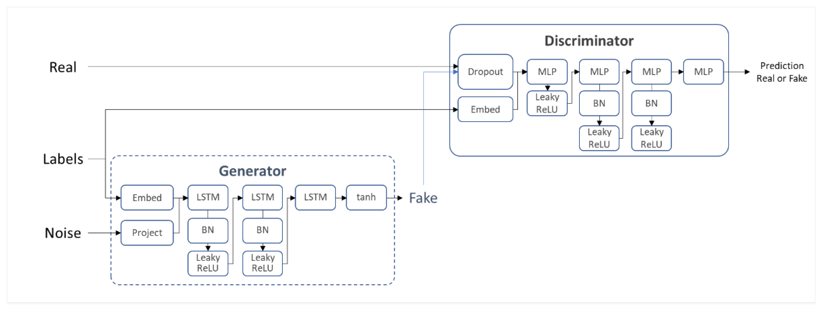
Conditional GAN is an extension of a GAN with a conditional variable $\mathit{y}$, which can be any extra information fed into both the Discriminator and Generator as an input layer [20,21]. As seen in Figure 1, random noise $\mathit{z}$, and the conditional variable, $\mathit{y}$, are concatenated in the hidden layer of the Generator to generate fake data ${\mathit{x}}^{\prime }$. This output of the Generator ${\mathit{x}}^{\prime }$, and the condition $\mathit{y}$, become an input for the Discriminator. The loss function is a min-max simultaneous optimization between the Discriminator and the Generator.

Synthetic data generation begins by setting the order of accounts as the condition $\mathit{y}$. For each subgroup, we train the Discriminator with the original data $\mathit{x}$, over its condition $\mathit{y}$, random noise $\mathit{z}$, and its condition ${\mathit{y}}^{\prime }$. Trained by the Discriminator, the Generator takes random noise $\mathit{z}$, and its condition ${\mathit{y}}^{\prime }$, as input and processes them to generate fake data ${\mathit{x}}^{\prime }$ and ${\mathit{y}}^{\prime }$, which become the input for the Discriminator. Then, the labeled data predicted as real by the Discriminator are converted back to the form of the original data.

3.3.1. Input Data Embedding

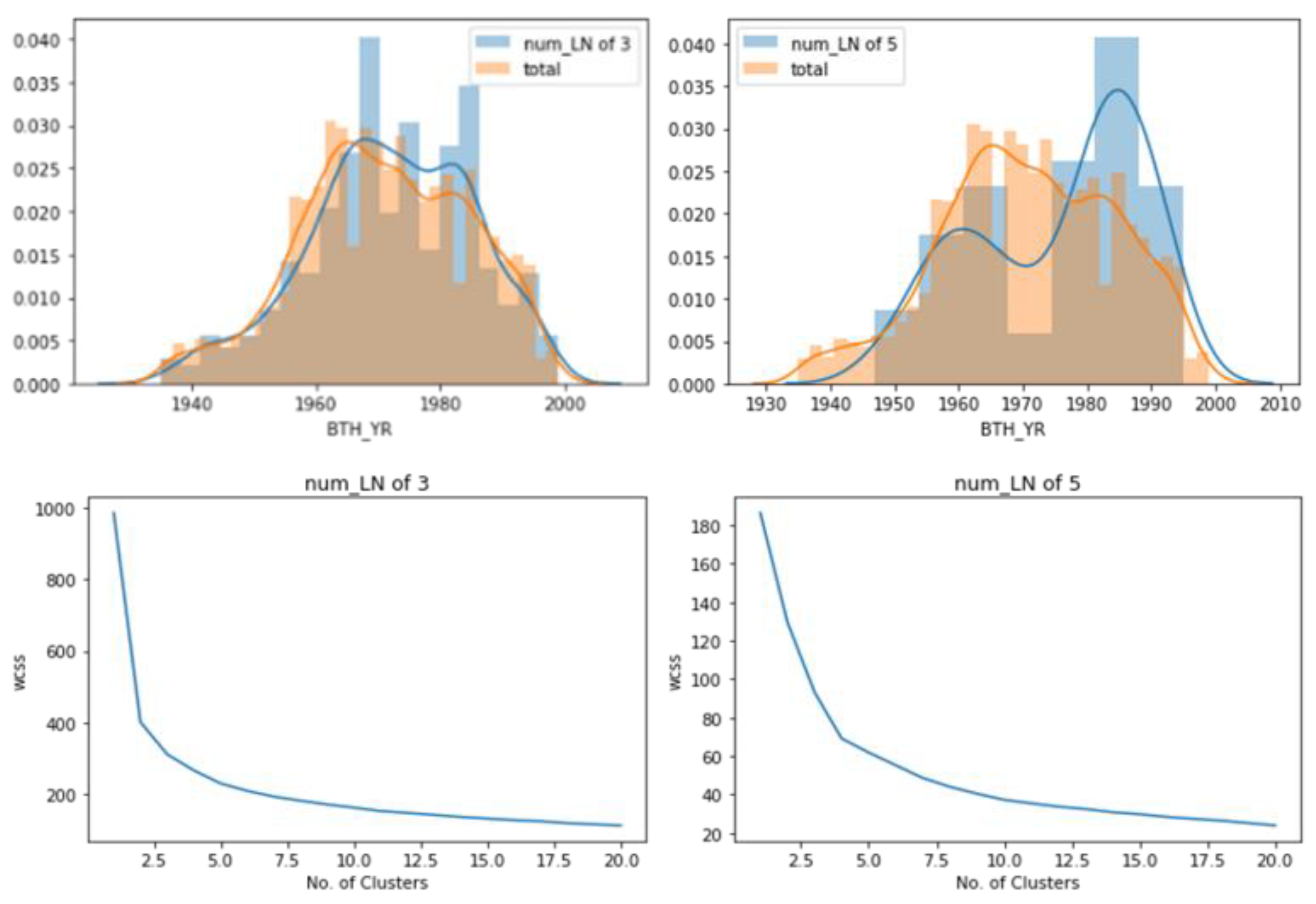
We have divided the dataset into seven subgroups to keep the patterns that might exist in those who have delinquencies and set the order of accounts as the conditional variable. As seen in Figure 2, the group with three loans seems to have most car owners in their late 30 s to 50 s. On the other hand, the group with five loans has most in their late 20 s and 50 s. A detailed discussion on this is beyond the scope of this paper, but it is clear that one′s financial activities are highly associated with one′s age, the type of the accounts, and its issue date and duration. With an assumption that the numerical variables are multimodal distribution, we estimate the number of modes and cluster the numerical variables using the Gaussian Mixture Model (GMM).

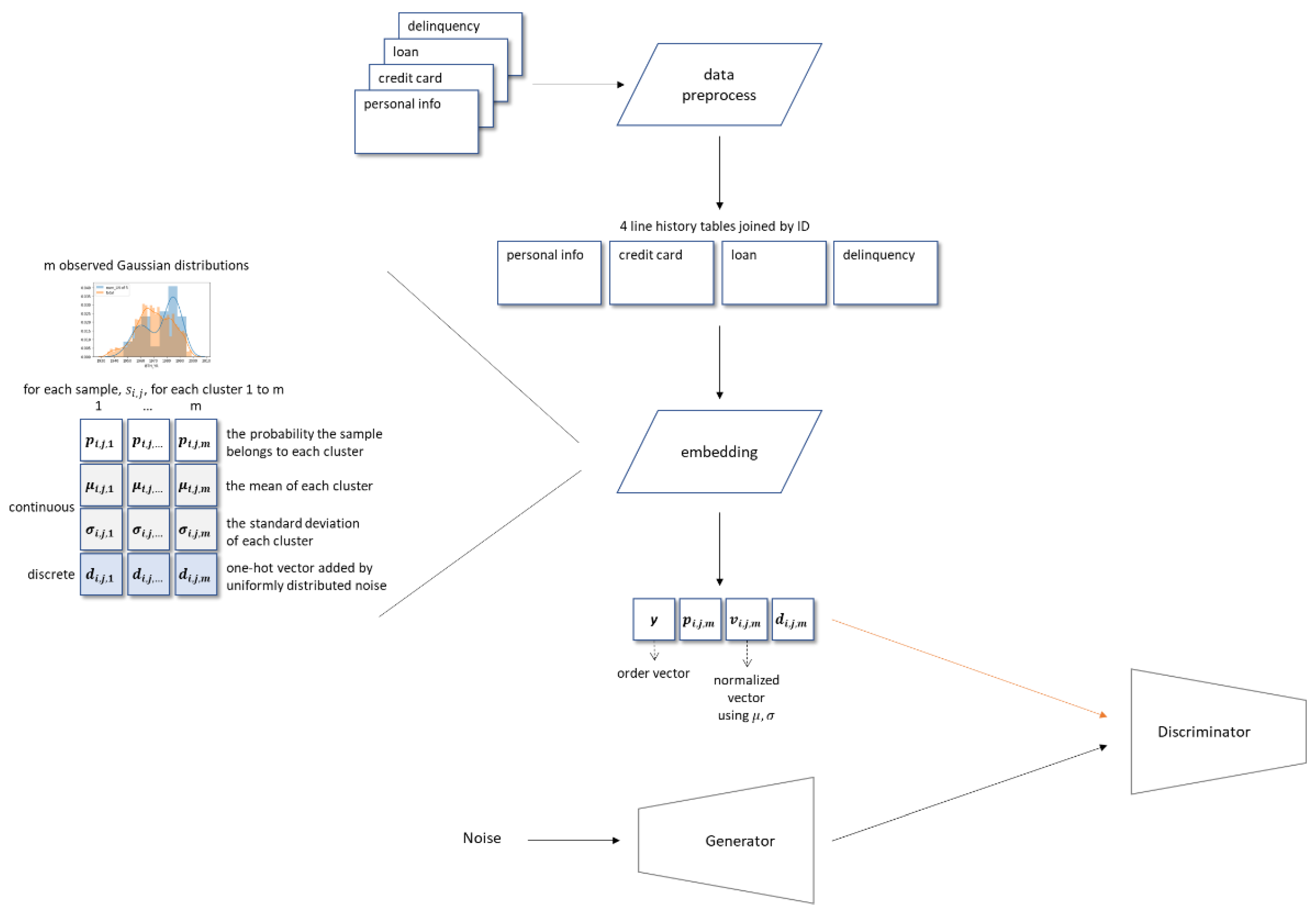
As described in Figure 3, we cluster the numerical variables using GMM as follows: first, set the probability that a sample $s_{i,j,1}, \cdots , s_{i,j,m}$, belongs to each cluster as $p_{i,j,1}, \cdots , p_{i,j,m}$, and the mean and standard deviation for each distribution as ${\mu }_{i,j,1}, \cdots , {\mu }_{i,j,m}$ and ${\sigma }_{i,j,1}, \cdots , {\sigma }_{i,j,m}$, respectively. Since $p_{i,j,1}, \cdots , p_{i,j,m}$ is a normalized probability distribution of the sum of $m$ Gaussian distributions, we normalize a sample $s_{i,j}$, as $v_{i,j}$, and finally, a numerical sample $s_{i,j}$, is denoted with a vector $p_{i,j}, v_{i,j}$. For categorical variables, we used a light version of Gumbel- SoftMax, adding a uniformly distributed noise to one-hot vectors to make them dense or differentiable [15,17,22]. A categorical sample $s_{i,j}$, after one-hot encoded and added by a noise drawn from a uniform distribution, is denoted as $d_{i,j}$.

Afterward, we rebuild the table by binding the column vectors in the form of $p_{i,j,1}, \dots , p_{i,j,m}, v_{i,j,1}, \dots , v_{i,j,m}, d_{i,j}$. This form applies to the output of the Generator, and it becomes an input for the Discriminator. Once labeled either real or fake, the vectors are converted back to the original form of data; for numerical variables $s_{i,j}= 2v_{i,j,k}{\sigma }_{i,j,k}+{\mu }_{i,j,k}$, where $k$ lies between 1 to $m$, inclusive; for categorical variables, by simply taking the index of the largest element of $d_{i,j}$.

3.3.2. Generator

The Generator takes the normalized vector $v_{i,j}$ and its cluster information vector $p_{i,j}$, as its input and predicts the probability distributions for categorical data, $d_{i,j}$. For subgroups with two or more accounts, we used LSTM as there is a causality. For example, the group with cards and loans had issued the credit card, then the loan occurred through the same account, or those with loans and delinquencies must have had outstanding loans before the account turned into delinquent. In any case, the balance may not be summed up to the preceding account. The inputs to each LSTM could be either a random vector $\mathit{z}$, $tanh\left(W_h{h}_{t-1}\right)$, or $tanh\left(W_h{h^{\prime }}_{t-1}\right)$, where $h_{t-1}$ is a hidden vector at $t-1$, ${h^{\prime }}_{t-1}$ is its embedding vector, and $W_h$ is the weight of the layer.

Figure 4 shows how the Generator is trained using the output of the Discriminator. The Generator itself does not yield the loss directly; in fact, its output feeds into the Discriminator, and the generator loss penalizes the Generator for generating data classified as fake. Weight adjustment begins with the Discriminator output goes back through the Discriminator into the Generator.

$${ℒ}_{\mathrm{G}}=E_{z~P_{Z\left(z\right)}}[log(1-D(G(\mathit{z}|\mathit{y})))]+\sum KL\left({\mathit{x}}^{\prime },\mathit{x}\right),$$

(1)

3.3.3. Discriminator

The structure of the Discriminator is a fully connected multilayer perceptron with an activation function of LeakyReLU for a weighted penalty and Adam optimizer. Trained with both the real and fake data with labels, it attempts to classify the incoming labeled data as real or fake out of the given batches of labeled data, containing both the randomly generated and the samples from the real data.

$${ℒ}_{\mathrm{D}}=E_{\mathrm{x}~P_{X\left(x\right)}}[log(D(\mathit{x}|\mathit{y}))\left]+E_{z~P_{Z\left(z\right)}}\right[log(1-D(G(\mathit{z}|\mathit{y})))],$$

(2)

3.3.4. Loss Function

We used Adam optimizer when training our model and added the optimized Kullback–Leibler (KL) divergence as a constraint so that it would converge more stably [19]. KL-Divergence, instead of cross-entropy, was used because it gives a relative distance in a mixture of categorical and clustered continuous variables. We compute the final objective function as follows by optimizing (1) and (2):

$$mi{n}_{G}ma{x}_D=E_{x~p_{X\left(x\right)}}\left[logD\left(\mathit{x}|\mathit{y}\right)\right]+E_{z~p_{Z\left(z\right)}}\left[log\left(1-D\left(G\left(\mathit{z}|\mathit{y}\right)\right)\right)\right]+\sum KL\left(x^{\prime },x\right),$$

(3)

It infers the probability of true or false when a dataset is assigned to a conditional variable $\mathit{y}$, which is the order of the accounts. Theoretically, KL divergence is not a distance but a measure for how two distributions are different. The concept is widely used as a distance measure because the more two distributions are different, the higher the divergence, and the divergence becomes 0 only when the two are identical. However, one should be aware of the fact that it is not symmetric ${\mathit{D}}_{\mathit{K}\mathit{L}}(\mathit{p}\parallel \mathit{q})\ne {\mathit{D}}_{\mathit{K}\mathit{L}}(\mathit{q}\parallel \mathit{p})$, where $\mathit{p}$ is the probability distribution of the original dataset, and $\mathit{q}$ is the probability distribution of a synthetic dataset.

4. Results

While other neural networks train with a loss function until it converges, GAN trains the Generator with the Discriminator classifying the outputs of the Generator as real or fake. As the evaluation of the Generator solely depends on the performance of the Discriminator, when the Discriminator fails, there is no way to assess the quality of the Generator objectively. Moreover, as Snoke et al. (2017) suggested, the agencies who provide the synthetic data will not know what analyses users would carry out and therefore, the utility measure should be analyses-specific [23]. For that reason, we first examined the statistical confidentiality and the normalized mutual information, then inspected how consistent the synthetic data compared to the original data using the analysis approaches credit ratings agencies practice. We also used a few standalone machine learning algorithms to predict delinquency and compared the confusion matrix and accuracy for data consistency.

4.1. Statistical Confidentiality

Snoke et al. (2017) introduces general statistical utility measures, including propensity scores and interval-overlap [23]. However, we concluded that in this consumer credit case, such statistical measures would not be sufficient considering exposure risks altogether. To be specific, previously known methods are applied to cross-sectional data, an observation on a sample at one given time, but consumer credit observes a group sample over a successive period. Even if the propensity scores and interval-overlap agree at 5% confidence interval, it does not necessarily mean that they are distributed accordingly to the corresponding period. Therefore, for the statistical confidentiality, we only compare the distributions of the attributes from the original and synthetic data to see if the model can generate the mixture of Gaussian distribution.

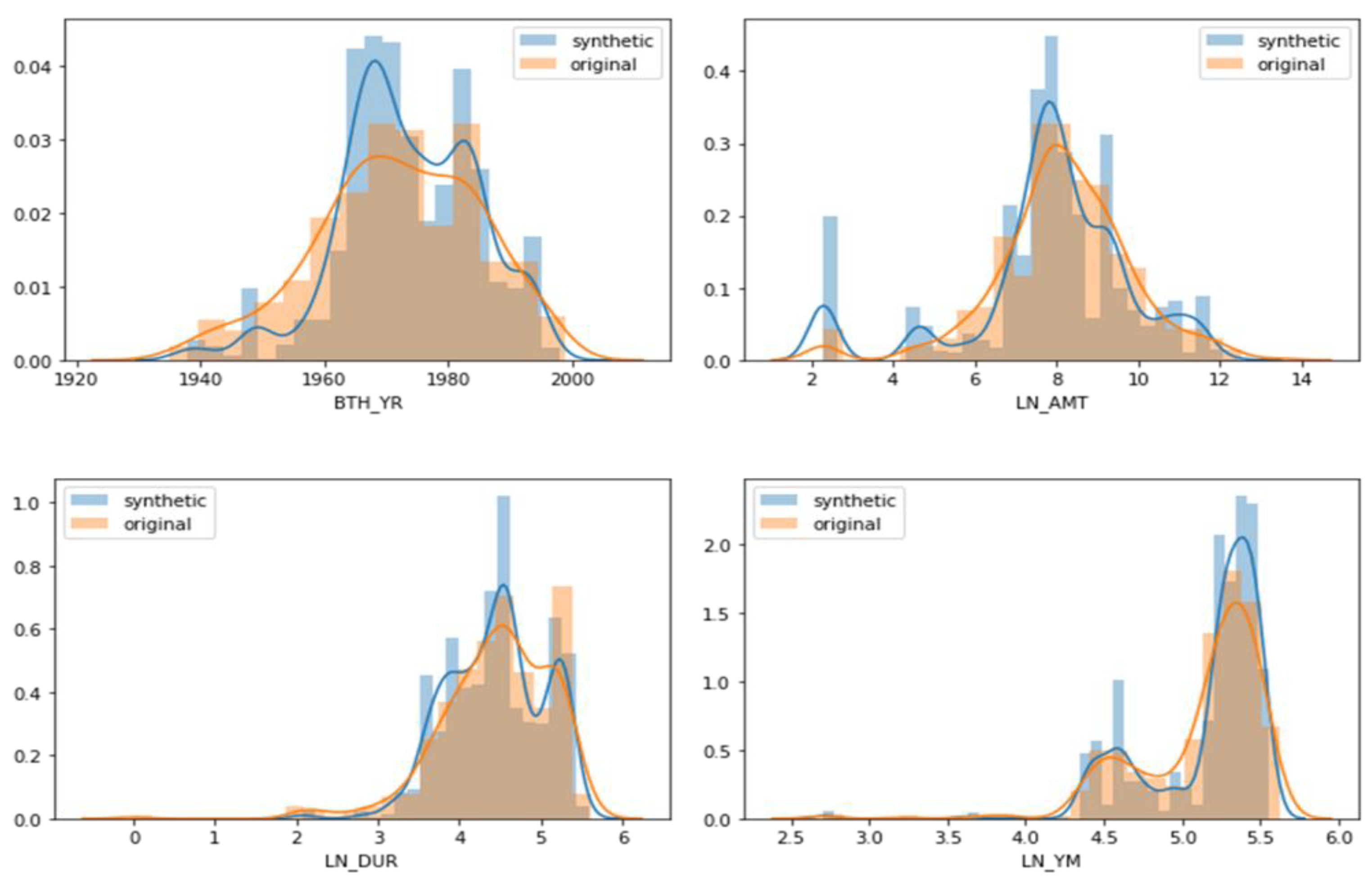
As shown in Figure 5, the distributions of attributes in the synthetic dataset fit very close to the distributions of the original dataset. It is also notable that they show sharper peaks than those in the original dataset. It seems to be that applying a GMM to data generation has highlighted its features of the multimodal distribution.

4.2. Normalized Mutual Information

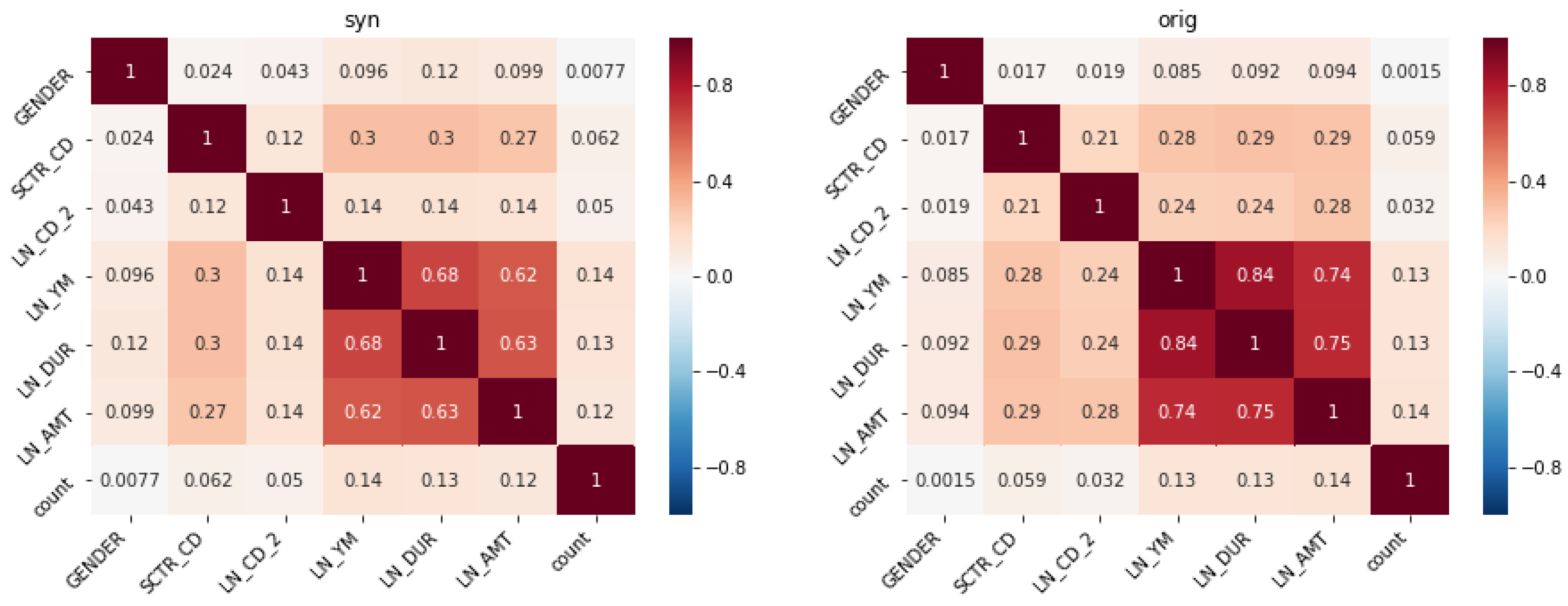
Next, we compared the Normalized Mutual Information (NMI), quantifying the mutual dependence between two random variables to scale between 0, where there is no mutual information, and 1, there is a perfect correlation. NMI normalizes two variables and measures the KL divergence between their joint distribution and their products, or marginal distributions. If two variables are independent, their joint probability is equal to the marginal distribution. Therefore, the divergence is 0, and there is no mutual information between them. As the KL divergence grows from zero, two variables are dependent; thus, they share mutual information.

Figure 6 shows the NMI of the group with three loans. While the term of the loan, set to either 0 or 1 depending on whether it is shorter than six months, shows relatively low mutual information, mutual information among the rest of the variables are well-reflected.

4.3. Data Consistency

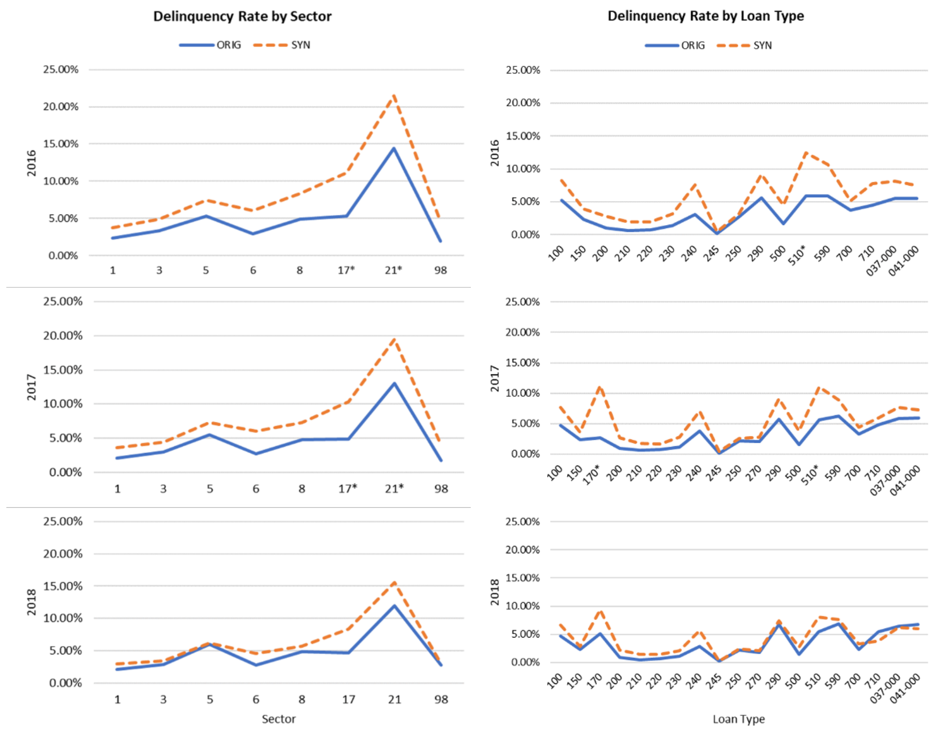
For data fidelity, we compared the percentage of overdue by sector, loan type, number of credit cards, and its holding period at the end of the years from 2016 to 2018. The left column of Figure 7 shows the delinquency rate by sector at the end of each year. The balances are relatively well maintained. The delinquency rate is quite higher than the original data; however, the synthetic dataset reflects the overall trends throughout the outstanding period. Sectors 17 and 21 are indicating third-tier financial institutions and savings banks, respectively. It seems to be that the number of unsecured loans made by third-tier institutions is relatively small and, therefore, difficult to predict its probability distribution more precisely.

The right column of Figure 7 shows the delinquency rate by loan types at the end of each year from 2016 to 2018, except for the loan type 170 and 510, which are loans for a lump-sum deposit for housing and used car mortgage, respectively, their trends are consistent with each other. Although the rate is slightly higher than the original dataset, the synthetic dataset replicates the overall trends throughout the outstanding period.

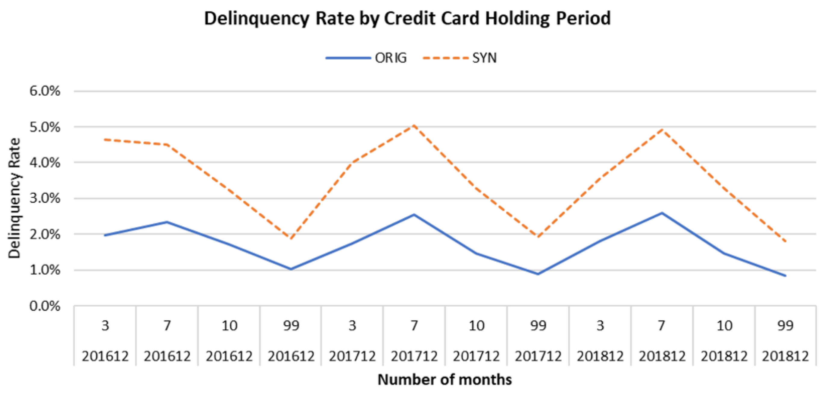
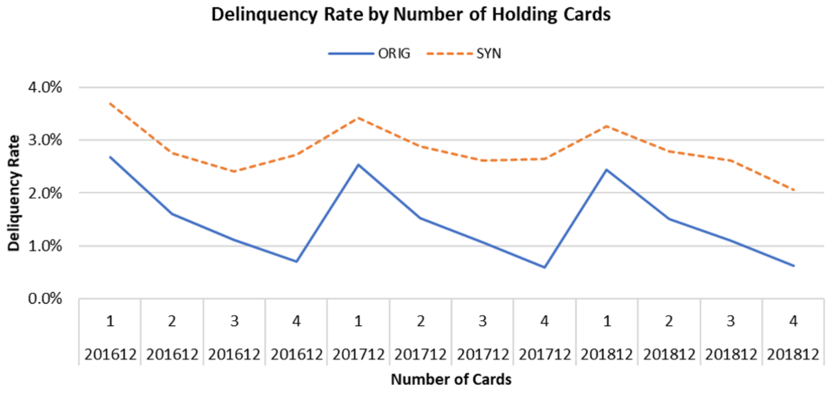
As seen in Figure 8 and Figure 9, the delinquency rates by the credit card holding period and the number of credit cards, respectively, from the synthetic dataset are higher than the original dataset. However, the overall trends are consistent with the original dataset.

We found that the delinquency rates are exaggerated throughout the period from 2016 to 2018, no matter under which condition. It seems to account for that the risk of delinquency is low in the early period and increasing throughout the whole period. We assume that the algorithm might have highlighted such features, ignoring rare cases, and emphasizing the regular ones.

In addition to this, we tried to evaluate the synthetic dataset using Logistic Regression, Decision Tree, and Support Vector Machine algorithms. Although those models are not generally used standalone to forecast or classify, for the scope of this study is to generate a dataset preserving the statistical properties of the original data, comparing the datasets using the above standalone models would suffice to say that the two datasets agree at a reasonable level. We created new columns—the number and amount of loans, non-bank loans, and collateral-free loans—for each car owner for predictor variables, as listed in

Table 3. Predictor variables to forecast delinquency.

Column	Description
num_NBLN_COM	Number of non-bank institutions
num_NCLN_COM	Number of institutions made unsecured loans
MAX_LN_DUR	The maximum loan outstanding period
MIN_LN_DUR	The minimum loan outstanding period
num_LN	Number of total loans outstanding
amt__LN	Total amount of loans outstanding
num_NBLN	Number of non-bank loans
amt_NBLN	Amount of non-bank loans
num_NCLN	Number of unsecured loans
amt_NCLN	Amount of unsecured loans
dlq	0 = Not delinquent loan, 1 = Delinquent loan

, since creditors, or models, should not discriminate against borrowers on a loan application or interest rates based on one′s characteristics such as age, sex, or race. The results show that the algorithm′s performances on original and synthetic datasets are considerably close enough that the synthetic dataset can be used as training data as in Figure 9.

Table 4. Confusion matrices for original and synthetic data.

Model	Data	Actual	Predicted 0	Predicted 1	Total
Logistic Regression	Original	Actual 0	709	191	900
		Actual 1	255	632	887
		Total	964	823	1787
	Synthetic	Actual 0	771	129	900
		Actual 1	321	566	887
		Total	1092	695	1787
Decision Tree	Original	Actual 0	675	225	900
		Actual 1	227	660	887
		Total	902	885	1787
	Synthetic	Actual 0	629	271	900
		Actual 1	281	606	887
		Total	910	877	1787
LDA (Latent Dirichlet Allocation)	Original	Actual 0	770	130	900
		Actual 1	287	600	887
		Total	1057	730	1787
	Synthetic	Actual 0	769	131	900
		Actual 1	328	559	887
		Total	1097	690	1787
Support Vector Machine	Original	Actual 0	732	168	900
		Actual 1	227	660	887
		Total	959	828	1787
	Synthetic	Actual 0	771	129	900
		Actual 1	305	582	887
		Total	1076	711	1787

shows the confusion matrices from the forementioned standalone machine learning algorithms. For each model, a confusion matrix with two rows and two columns reporting the number of true negative, false positive, true positive, and false negative, respectively from top left, clockwise. The synthetic dataset tends to yield more correct prediction on the loans that are not delinquent while yielding more wrong prediction on the loans that are delinquent than the original data. It indicates that the synthetic data has selected and generated the features of non-delinquent loans better than it has on the features of delinquent loans.

Finding a significant difference between two confusion matrices could be not only difficult, but risky as uninformative as it can be. A statistical difference might advise one cell of the matrix is different but does not provide enough information which metric or metrics are different. Therefore, we used standard approach that uses a single value metric to reduce each matrix into one value, and then to compare the values. Table 4 compares the same model on different datasets, the original and synthetic data, using precision, recall, and F1 metrics. Not to mention that we are not trying to compare the performance of the algorithms, but how algorithms work on two different datasets and check if they yield similar performance. Precision is the ratio of the actual delinquent loans to the loans that are predicted to be delinquent. Once a loan is predicted to be delinquent, the agency should start managing it by reminding the borrowers or offering other payment methods with lower interest rates, which are costly. Recall measures how many of the loans that are delinquent over the loans that are predicted not to be delinquent. Although this seems to be the situation most agencies want to avoid, higher recall does not always come before higher precision in this case for banks would not want to miss customers by rejecting a loan. To get a tradeoff between precision and recall, we use their harmonic mean, or F1-Score. In

Table 5. Forecast accuracy comparison.

Model	Data	Actual	Precision	Recall	F1-Score	Support
Logistic Regression	Original	Actual 0	0.74	0.79	0.76	900
		Actual 1	0.77	0.71	0.74	887
	Synthetic	Actual 0	0.71	0.86	0.77	900
		Actual 1	0.81	0.64	0.72	887
Decision Tree	Original	Actual 0	0.75	0.75	0.75	900
		Actual 1	0.75	0.74	0.74	887
	Synthetic	Actual 0	0.69	0.70	0.70	900
		Actual 1	0.69	0.68	0.69	887
LDA (Latent Dirichlet Allocation)	Original	Actual 0	0.73	0.86	0.79	900
		Actual 1	0.82	0.68	0.74	887
	Synthetic	Actual 0	0.70	0.85	0.77	900
		Actual 1	0.81	0.63	0.71	887
Support Vector Machine	Original	Actual 0	0.76	0.81	0.79	900
		Actual 1	0.80	0.74	0.77	887
	Synthetic	Actual 0	0.72	0.86	0.78	900
		Actual 1	0.82	0.66	0.73	887

, the F1-Score is no more than 5% point in all models for each category, 0 and 1. We conclude that the synthetic data could be used for training in developing machine learning models without distortion of reality.

4.4. Disclosure Risk

Soria-Comas (2017) explains the trade-off between overfitting and variance in data utility and disclosure risk [24]. In this, differential privacy is a relative measure that guarantees a similar variation in the neighboring datasets. As synthetic data mimics the original dataset distribution more closely, the errors would be lesser, or the disclosure risk would increase.

Fully synthesized data, where there is no direct mapping between real and synthetic datasets, disclosure risks are considered low since each combination of variables in fully synthetic data does not correspond to any individual. Moreover, even if an identical row is observed, it does not guarantee that the record belongs to an individual unless the rest of the individual′s historical data must be consistent as well.

Also, the original dataset used for this study had already been de-identified for privacy issues; the number of the unique records identically generated would be the exposure risk measure [25,26]. Out of over 1.7 million car owners, 843 car owners′ records, or 0.049%, matched the original records identically and uniquely. Among them, 88.3% were the credit card records only, most of which have a very low probability of re-identification.

5. Conclusions

We generated synthetic consumer credit data with the order of accounts as a condition. The results show that the univariate and multivariate distributions of the synthetic dataset are more peaked than the original dataset due to GMM. NMI comparison shows that the mutual dependence among the variables is similar. The prediction of delinquency using standalone machine learning algorithms worked at a comparable level. Finally, the data fidelity shows that the overdue difference is within 5% points with consistent trends. Besides, the exposure risk as low as 0.05%, which would not deteriorate the sample, the synthetic consumer credit data generated using GAN could be a useful resource for big data training programs in financial sectors.

It remains to note that this paper does not cover the individuals′ accounts as the time-series data other than setting the order of accounts as a condition. In other words, we assumed that consumers’ economic activities would show similar patterns such as the age range they first open an account or their first loan and its purpose. Future work should focus on clustering the samples into consumer groups to strengthen the assumption. Moreover, inspired by Papadopoulos et al. (2019), we continue working on rearranging individuals′ records as layers and generating compositional layer-based synthetic data [27,28]. Another limitation of our study is that we consider the uniqueness of individuals’ records as the exposure risk measure. As introduced in Jordan (2019), we plan to apply the differential privacy algorithm to the extent of a pre-determined threshold for disclosure risk and data post-process [29,30].