Smart Fibrous Structures Produced by Electrospinning Using the Combined Effect of PCL/Graphene Nanoplatelets

Abstract

Over the years, the development of adaptable monitoring systems to be integrated into soldiers’ body gear, making them as comfortable and lightweight as possible (avoiding the use of rigid electronics), has become essential. Electrospun microfibers are a great material for this application due to their excellent properties, especially their flexibility and lightness. Their functionalization with graphene nanoplatelets (GNPs) makes them a fantastic alternative for the development of innovative conductive materials. In this work, electrospun membranes based on polycaprolactone (PCL) were impregnated with different GNPs concentrations in order to create an electrically conductive surface with piezoresistive behavior. All the samples were properly characterized, demonstrating the homogeneous distribution and the GNPs’ adsorption onto the membrane’s surfaces. Additionally, the electrical performance of the developed systems was studied, including the electrical conductivity, piezoresistive behavior, and Gauge Factor (GF). A maximum electrical conductivity value of 0.079 S/m was obtained for the 2%GNPs-PCL sample. The developed piezoresistive sensor showed high sensitivity to external pressures and excellent durability to repetitive pressing. The best value of GF (3.20) was obtained for the membranes with 0.5% of GNPs. Hence, this work presents the development of a flexible piezoresistive sensor, based on electrospun PCL microfibers and GNPs, utilizing simple methods.

1. Introduction

The development of innovative smart microfibrous structures is in constant growth, owing to its versatility and wide range of applications, fundamentally due to its flexibility and ability to adapt to different shapes and surfaces [1]. Flexible technologies have the potential to be used for the construction of several structures, especially for the development of strain, pressure, temperature, humidity, and magnetic sensors [2]. These flexible, stretchable, and adaptable sensors are acquiring increasing attention in military area in order to make the soldier’s equipment smarter and safer without compromising its comfort and weight [3]. In fact, real-time vital signs and health monitoring of soldiers in the battlefield is essential to enhance their safety, requiring reliable and scalable systems [4]. There are many examples of smart systems incorporated onto textiles using hardware, such as cables and electronic components, that make them uncomfortable for the users. Thus, effort has been made to give fibrous structures themselves electrical properties without adding extra electronical materials to the textiles [5,6]. In this sense, researchers are continuously working on developing innovative fibrous structures with these kinds of characteristics [7]. Micro/nanofibers produced by electrospinning are one of the most interesting, versatile, and advantageous structures in this area, considering their remarkable characteristics such as high surface-volume ratio, high porosity, lightness, and high flexibility [8,9].

In recent years, biopolymers, such as polycaprolactone (PCL), have emerged as a great sustainable option due to their low cost, biodegradability, and availability [10]. Besides being one of the most used biopolymers for the production of electrospun fibers, PCL also presents other favorable features, such as cost effectiveness, simplicity of fabrication, and ease of operation [11,12].

The functionalization of electrospun microfibers with nanoparticles is one of the strategies used for the development of innovative materials with enhanced intelligent and multifunctional properties, avoiding the addition of extra weight onto the systems [13,14]. Functionalization with carbon-based nanoparticles opens up a new horizon of opportunities to create electrical conductive networks, which are essential to obtain a piezoresistive behavior (variation in electrical resistance during compression). Piezoresistive sensors can be used for dynamic and static pressure measurements [15,16].

Graphene has become one of the most studied carbon-based materials in recent years due to its excellent mechanical characteristics and thermal and electrical conductivity properties [17]. The main limitations of pure graphene are low fabrication rates and high cost. Hence, graphene nanoplatelets (GNPs) can be an excellent alternative that solves those issues, combining large-scale production and low cost [18,19]. Therefore, the addition of GNPs to an electrospun membrane turns them into ideal candidates for pressure-sensing applications due to their combined properties, particularly their large stretchability and electrical conductivity [20]. Several examples in the literature have presented the high potential of GNPs for the development of flexible electronic devices. Recently, Baloda et al. [21] developed a flexible resistive-strain sensor based on GNPs/polydimethysiloxane (PDMS), providing good strain sensitivity for human motion detection and health monitoring applications. Sabzi et al. [22] also prepared a flexible nanocomposite of GNPs and poly(lactic acid) (PLA) with electrical conductivity properties. Lu et al. [23] produced a flexible sensor with GNPs and epoxy with controllable sensitivity and linearity.

There are also several examples in literature that have reported the use of GNPs in flexible textiles, showing their potential in flexible textile technology. High sensitive damage sensors based on glass fiber fabrics coated with functionalized GNPs were developed by Moriche et al. [24]. Pereira et al. reported the development of a piezoresistive sensor based on the combined effect of GNPs, flax fabrics, and biopolymers, such as chitosan and polyethylene glycol [6]. Souri et al. also developed flexible and wearable strain sensors by the coating of flax fabrics with GNPs using the ultrasonication technique [25]. However, the incorporation of the GNPs into the microfiber membranes still represents a challenge. In some cases, it is difficult to ensure a proper distribution of the GNPs onto the membranes, which strongly influences their final electrical properties. Therefore, the use of the post-modification method for electrospun membrane impregnation appears to be an alternative to improve the homogeneity, adhesion, and stability of GNPs at the fibers surface. [26]. Hence, the main goal of this study was to develop a very flexible smart material based on GNPs and PCL electrospun membranes with excellent and stable electrical properties for potential application as piezoresistive sensors. First, the polymeric solutions and electrospinning parameters were optimized in order to produce defect-free PCL electrospun microfibers. In parallel, several GNPs solutions with different GNPs concentrations were optimized using ethanol as solvent. Then, the electrospun PCL membranes were immersed into the GNPs dispersions and dried after the impregnation. The developed systems were properly characterized through Raman Spectroscopy, Field Emission Scanning Electron Microscopy (FESEM), and Thermogravimetric Analysis (TGA). The electrical performance of the developed systems was studied, including the evaluation of the electrical conductivity properties, piezoresistive behavior (changes in the electrical resistance of the material caused by mechanical deformations), and their Gauge Factor (GF).

2. Materials and Methods

2.1. Materials

PCL (with a molecular weight of 80,000 g/mol, Tm = 60 °C, density = 1.145 g/mL at 25 °C, Sigma Aldrich, St. Louis, MO, USA) was utilized. The solvents used were Chloroform (CHF, 99.0–99.4% Normax, Marinha Grande, Portugal), N,N-Dimethylformamide (DMF, 99.99% Fisher Scientific, Leics, UK), and Ethanol (96% Normax, Marinha Grande, Portugal). The Elicarb^® GNPs powder materials grade (multilayered graphene platelets with typical lateral size of 5 µm and surface area between 30–50 m²g⁻¹) was provided by Thomas Swan & Co. Ltd., Rotary Way, Consett, Durham, UK.

2.2. Production of Electrospun PCL Membranes

To produce all the samples for this work, several steps were performed. First, the polymeric solutions were optimized, varying the PCL concentration. The electrospinning parameters were also optimized in order to obtain homogeneous fibers in distribution and diameter. Finally, the electrospun membranes were impregnated with several GNPs solutions to obtain the final system. A schematic flow chart of the whole process is represented in Figure 1.

2.2.1. Preparation and Optimization of the PCL Polymeric Solutions

In order to produce defect-free microfibers, the polymeric solutions were optimized, varying the PCL concentration. Several PCL formulations were prepared using 15%, 20%, and 25% (w/v) of PCL in CHF/DMF (4:1) [22,27]. First, PCL pellets were introduced slowly to CHF and stirred at 35 °C for at least 3 h (until a clear solution was achieved). Then, DMF was incorporated to the polymeric solution after the PCL was completely dissolved [28] and stirred for another 24 h.

2.2.2. Electrospinning Process

Electrospun membranes were produced using the electrospinning equipment NF-103 from MECC Co., Ltd. (Fukuoka, Japan) and conducted by transferring the polymer solution into a 12 mL plastic syringe (NORM-JET^®, Henke Sass Wolf, Germany) with an orthogonally cut-ended needle (20 GA GP 023X1.0 Pink 50PC, Nordson EFD, OH, USA).

The electrospinning parameters were also optimized, including the distance between the collector and the needle, the applied voltage, and the polymeric solution flow rate, in order to obtain the most homogenous fibers as possible. For this work, the ranges evaluated were from 240 mm to 260 mm for the collector-needle distance, between 25 kV and 29 kV for the voltage, and from 1 mL/h to 5 mL/h for the flow rate. After the optimization of the polymeric solutions and the electrospinning parameters, the production of PCL microfibers was performed using a drum collector and a deposition time of 5 h.

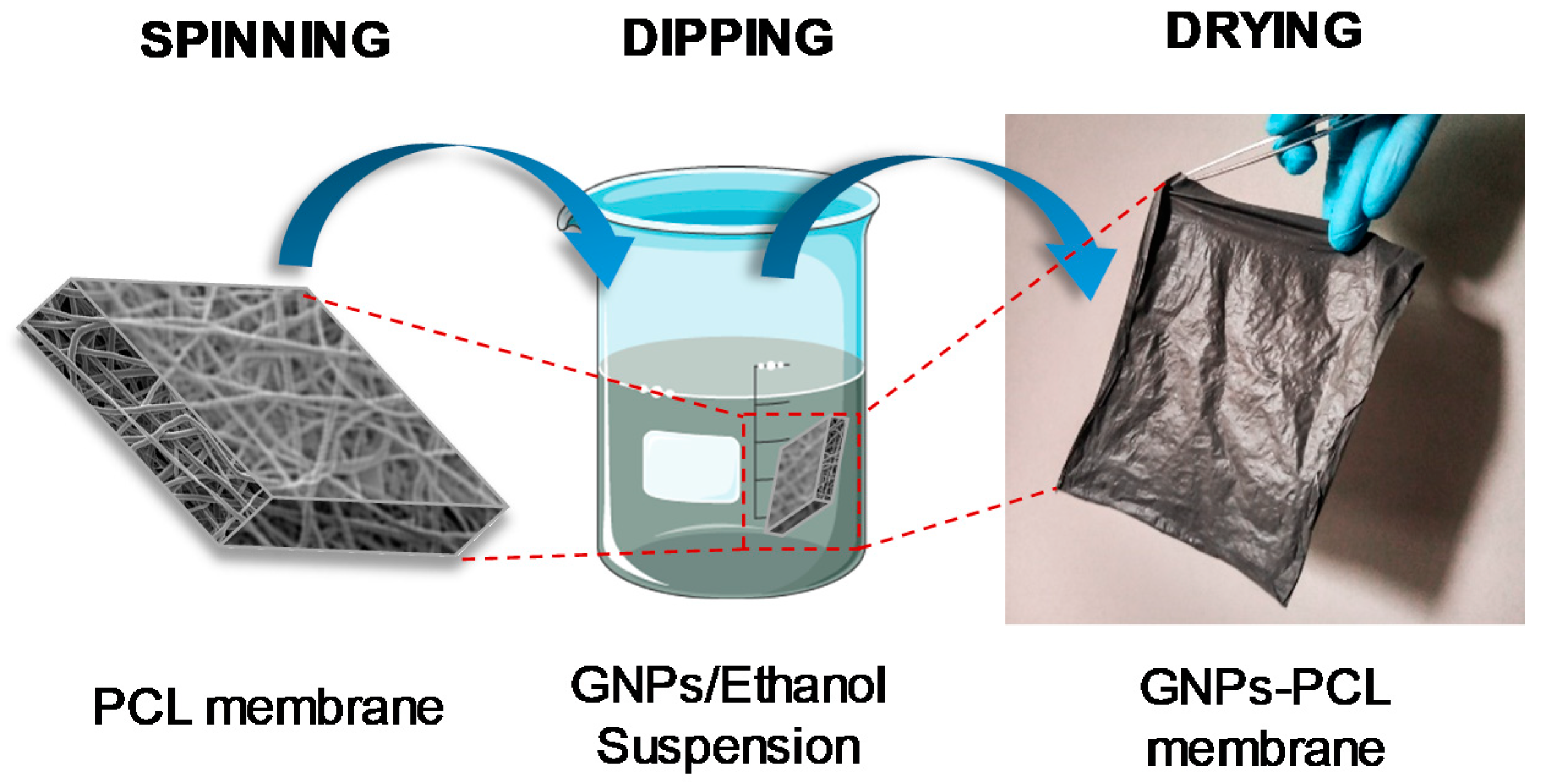
2.2.3. Preparation of the GNPs-PCL Membranes

In order to incorporate the GNPs onto the PCL electrospun membranes, several solutions with different GNPs concentrations (0.05, 0.1, 0.2, 0.5, 1 and 2% (w/v)) were prepared. GNPs powder was dispersed in ethanol and kept under magnetic stirring for 4 h using 350 rpm at room temperature. Then, the solution was placed in an ultrasound bath (Sonica Ultrasonic Cleaner, Soltec, Italy) for another hour at room temperature. Then, the PCL electrospun membranes were cut into 160 mm × 200 cm rectangles, immersed in the solution of GNPs, and stirred by an orbital shaker (Ivymen System, Comecta, Spain) at 120 rpm for 5 min, 15 min, 30 min, and 60 min in order to evaluate the influence of the immersion time in the GNPs adsorption. Subsequently, GNPs-PCL membranes were taken out of the previous solutions and dried at room temperature. The membranes were then subjected to a treatment of 5 consecutive cycles of washing (with distilled water for 1 h each) and drying at room temperature to remove the superficial excess (water treatment cycles), using an adaptation of the ISO 6330:2012 standard “Textiles-Domestic washing and drying procedures for textile testing. Based on the GNPs content in the impregnation solutions, the membranes were named as 0.05%GNPs-PCL, 0.1%GNPs-PCL, 0.2%GNPs-PCL, 0.5%GNPs-PCL, 1%GNPs-PCL, and 2%GNPs-PCL. PCL membrane dipped in an ethanolic solution was used as control.

The GNPs loading mass of GNPs-PCL membranes was determined by the Formula (1):

$${\mathrm{m}}_{\mathrm{GNPs}}={\mathrm{m}}_{\mathrm{GNPs}/\mathrm{PCL}\mathrm{membrane}}-{\mathrm{m}}_{\mathrm{PCL}\mathrm{membrane}}$$

(1)

where mGNPs, mGNPs/PCL membrane, and mPCL membrane refer to the GNPs loading mass, the quantity of the PCL membrane with GNPs, and the quantity of the PCL membrane, respectively.

2.3. GNPs-PCL Membranes Characterization

2.3.1. Field Emission Scanning Electron Microscopy (FESEM)

An exhaustive morphological analysis of the membranes was made through an ultra-high resolution FESEM, NOVA 200 Nano SEM, FEI Company (Hillsboro, OR, USA). Before the analysis, the samples were covered with a very thin film (20 nm) of Au-Pd (80–20 wt%), using a high-resolution sputter coater, 208 HR Cressington Company (Watford, UK), coupled to an MTM-20 Cressington High Resolution Thickness Controller. The diameters of electrospun microfibers were determined using Image J software. The FESEM images of the samples were analyzed, and the diameters were measured in 100 different locations.

2.3.2. CIELAB Color Coordinates

To evaluate the homogeneity of the GNPs distribution all over the samples’ surfaces, 5 random points of each sample were measured by a Datacolor spectrophotometer using the difference Cielab coordinates D65/10 software (Lucerne, Switzerland). The L* parameter was measured in order to give information about the difference in lightness of the membranes, which is the most important coordinate for this type of samples (with colors on the grey scale).

2.3.3. Thermogravimetric Analysis (TGA)

Thermogravimetric Analysis (TGA) was carried out using a STA 700 SCANSCI in order to study the influence of the GNPs incorporation on the membranes’ degradation temperature. The TGA trace was obtained in the range of 25–600 °C, under nitrogen atmosphere, with a constant heating rate of 20 °C/min. The percentage of GNPs was calculated using the following system of equations [4]:

$$\{\begin{array}{c}\mathrm{GNPs} \%+\mathrm{PCL} \mathrm{membrane} \% \left(\frac{\mathrm{PCL}\mathrm{membrane}\mathrm{residues}\%}{100}\right)=\mathrm{sample} \mathrm{total} \mathrm{residues} \% \\ \mathrm{GNPs} \%+\mathrm{PCL} \mathrm{membrane} \% =100 \%\end{array}$$

(2)

2.3.4. Raman Spectroscopy

Raman spectroscopy is an analytical and nondestructive technique that studies the structure and composition of a sample through the identification of its vibrational modes [28]. This technique was used to analyze the structure of the GNPs used. Raman spectra were obtained on a Horiba LabRAM HR Evolution microscope (Horiba Scientific, Longjumeau, France) equipped with a 532 nm (2.33 eV) laser. A 100× objective lens was used to focus the laser onto the samples. The results were analyzed using the LabSpec 6 software (also from Horiba Scientific). For each sample, an average of 4 scans was collected at random places of the samples’ surface, in order to ensure the analysis’ homogeneity.

2.4. Functional Properties Evaluation

2.4.1. Electrical Conductivity

To evaluate the electrical conductivity, it was necessary to measure the electrical resistance of the material using an electrical source, which was connected to the material by conductive electrodes (2-wire method). Using this method, the electrical resistance was obtained through the I-V curves (electric current intensity–voltage applied) [29].

The electrical resistivity $\rho$ (Ω·m) was calculated by the Equation (3):

$$\rho =R\times \frac{A}{L}$$

(3)

where R is the electrical resistance, A is the cross-sectional area of the electrode (mm²), and L is the distance between the electrodes (mm). The electrical conductivity is given by the inverse of the electrical resistivity [29].

Electrical resistivity is defined as the capacity of a given material to resist the flow of electric current intensity. In general, the electrical resistivity is inversely proportional to the electrical conductivity, as represented in Equation (4) [30]:

$$\sigma =\frac{1}{\rho ’}$$

(4)

where $\sigma$ represents the electrical conductivity (S/m) and $\rho$ the electrical resistivity (Ω·m).

For this work, electrical resistance measurements were performed using a Keithley 6487 Pico-ammeter/Voltage source by applying a potential difference in a range between −1 to 1 V, with a step of 0.1 V. All measurements were performed in direct current (DC) mode at room temperature. In order to determine the electrical resistance through the current intensity measurements, an electrode system with a cross-sectional area of 5 × 1 mm² and a distance between electrodes of 3 mm was developed. Equation (3) was utilized to obtain the electrical resistivity, as the electrical resistance was determined by the slope of the I-V curves. Then, Equation (4) was applied in order to obtain the electrical conductivity values. The electrical resistance was measured in 5 different places of the sample, and the average value was calculated.

2.4.2. Piezoresistive Behavior

For the piezoresistive behavior evaluation, we simultaneously used a Hounsfield tensile test equipment with a 250 N load cell, with a 0.04 mm Z-axis deformation, and a compression speed of 0.08 mm/min over the sample in a circular surface, with a diameter of 10 mm, for 10 cycles. Simultaneously, to measure the variation of electrical resistance, 2 electrodes were placed on the clamps, as shown in the scheme of Figure 2. Through these electrodes connected to a digital multimeter (Agilent 34461A), it was possible to measure and record the variation in electrical resistance over the 10 compression cycles.

The piezoresistive effect of the membranes can be determined by calculating their mechanical deformation (ε) and their corresponding electrical resistance variation (ΔR) [31]. The mechanical deformation was determined as the ratio between the transverse deformation (mm) and the initial thickness of the sample (mm).

For this test, overlapping a known number of layers of the analyzed membrane was necessary. Then, ΔR was determined according to Equation (5):

$$\Delta R=\left(R-R_0\right)$$

(5)

where R represents the electrical resistance in a time t and R₀ the initial electrical resistance (at time 0). Then, the behavior curves were analyzed in the same graph to study the relationship between the mechanical deformation and the electrical resistance variation of the material over time. Finally, the GF, which determines the sensitivity of a piezo resistor (the fractional change in the resistance per unit strain), was calculated as follows:

$$GF=\frac{\raisebox{1ex}{$\Delta R$}\!\left/ \!\raisebox{-1ex}{$R_0$}\right.}{\epsilon }$$

(6)

3. Results

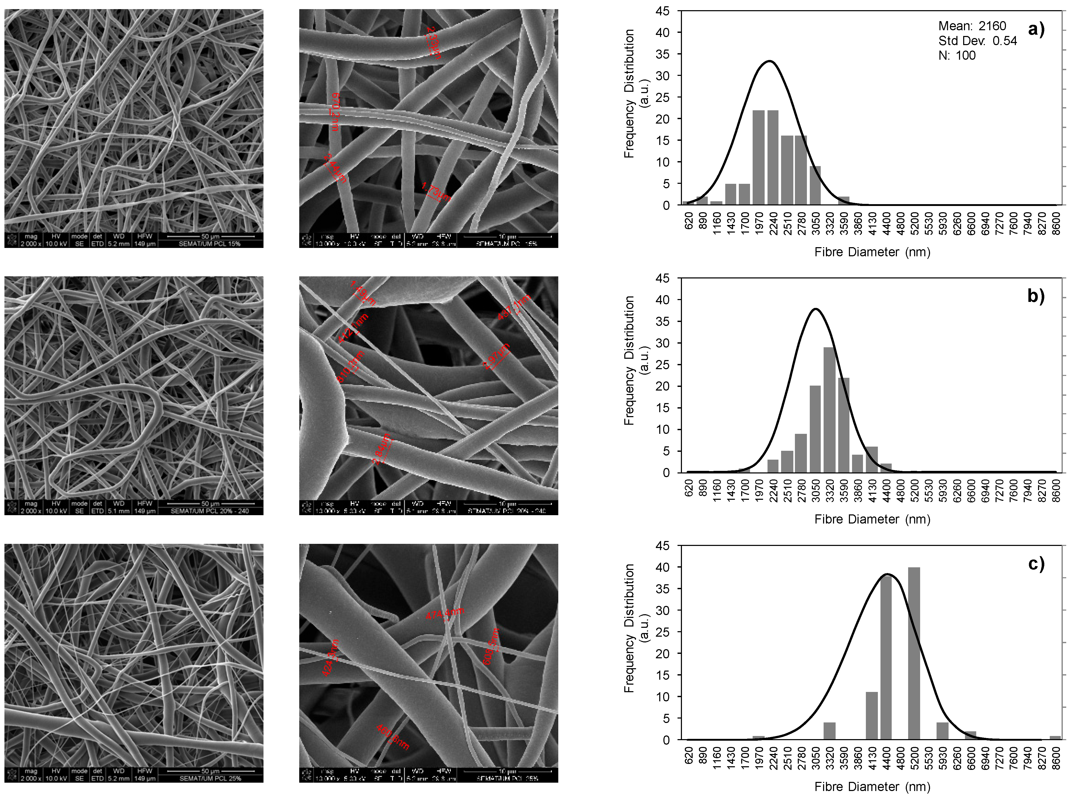
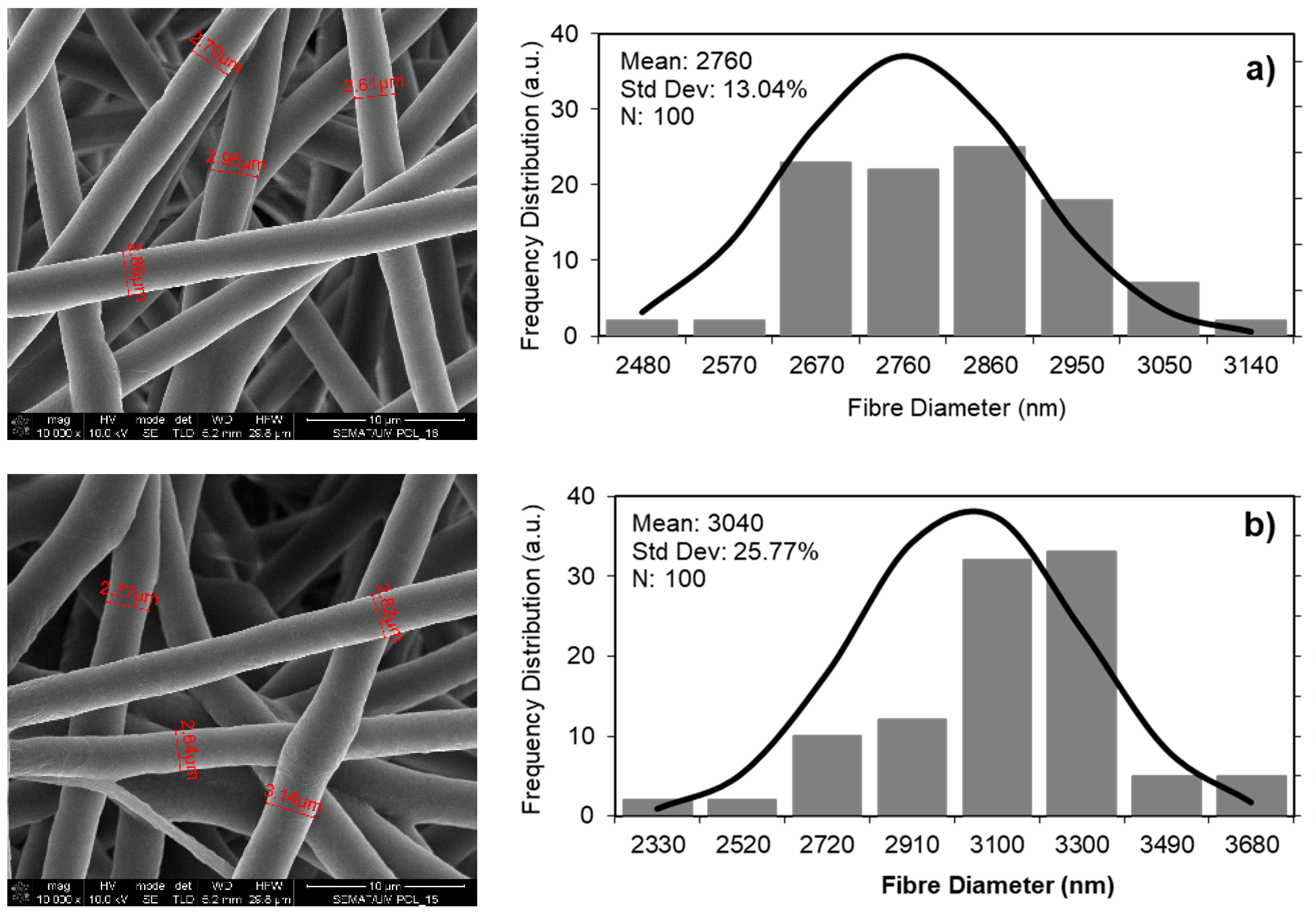
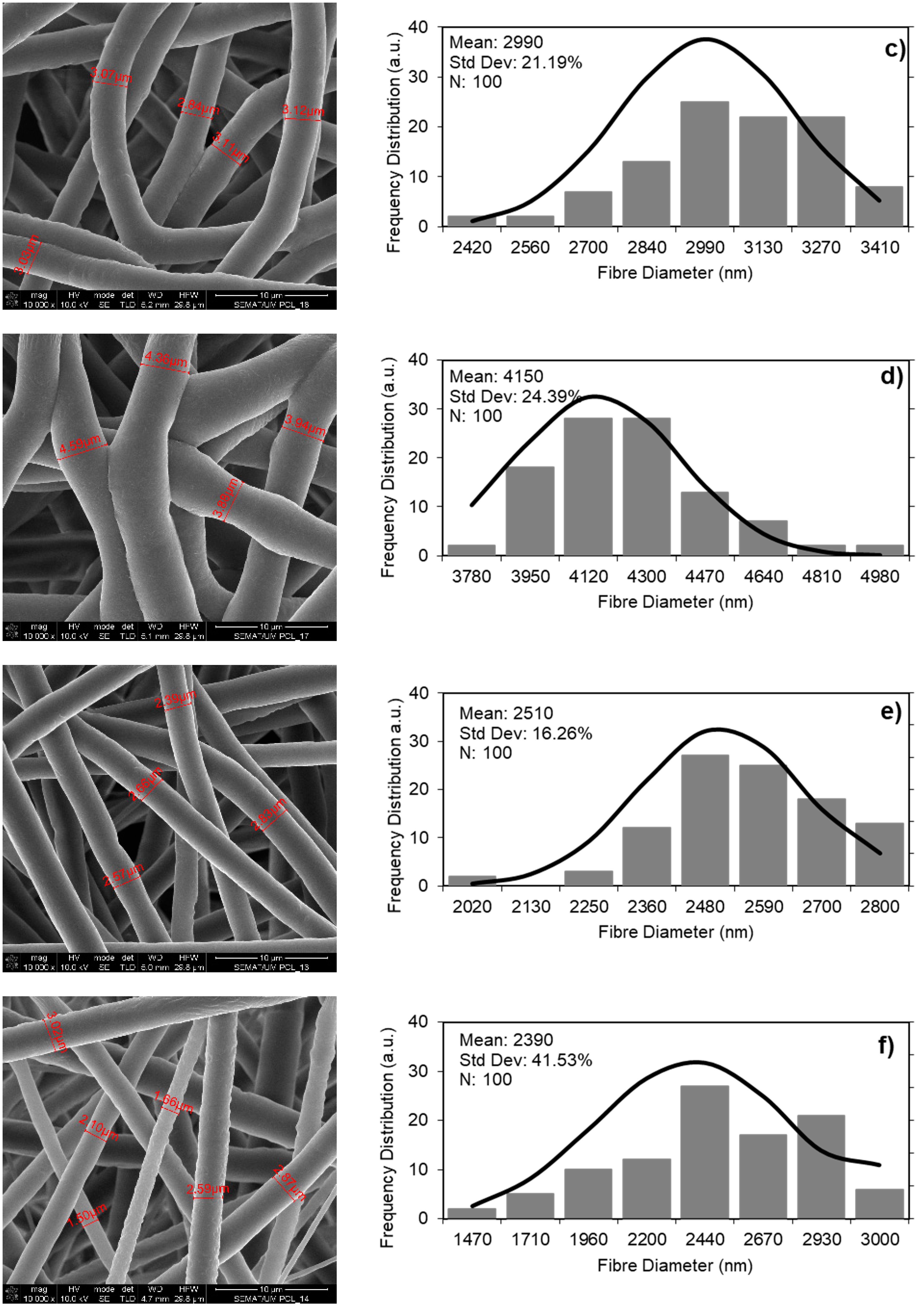
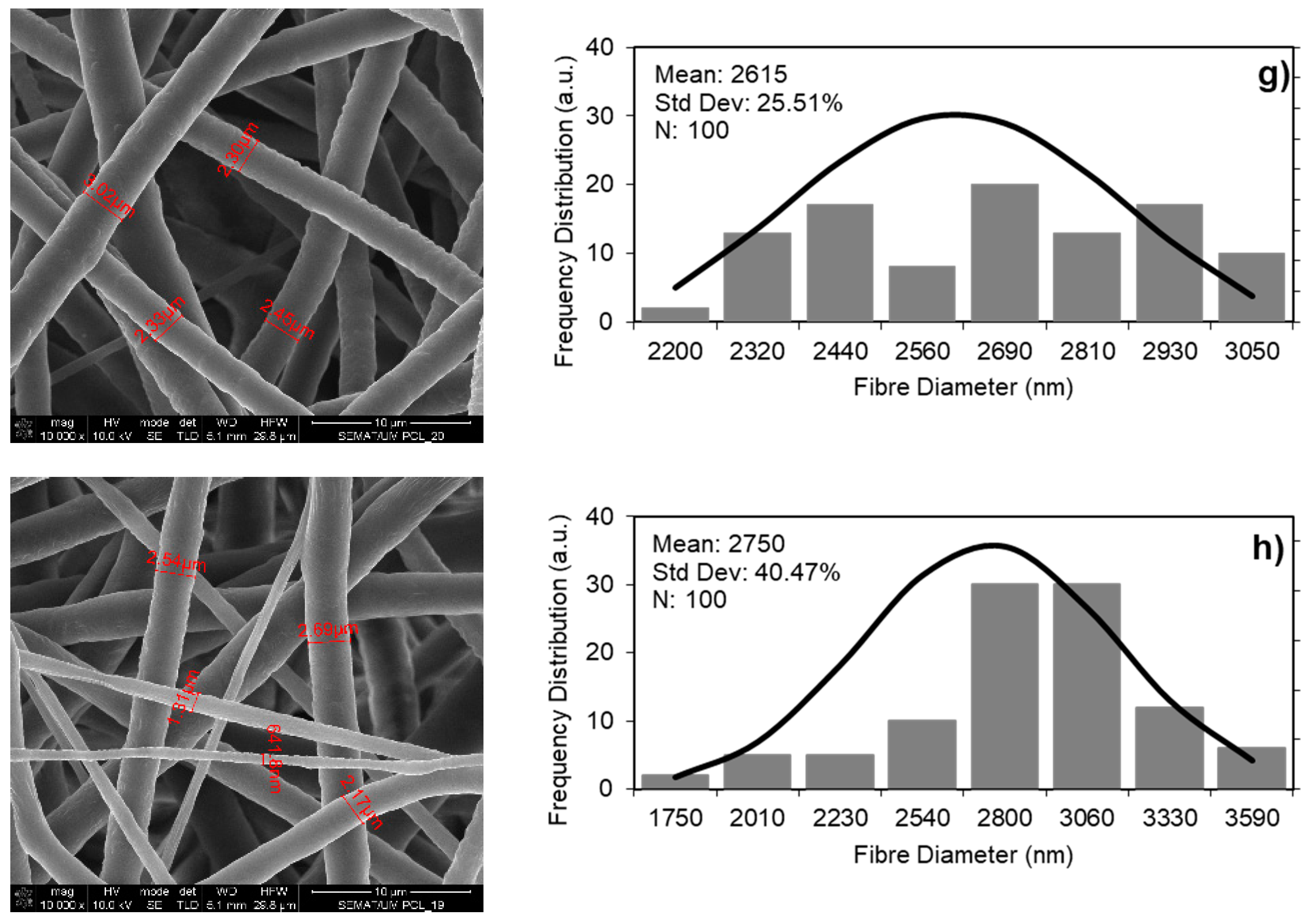
3.1. PCL Polymer Solution, Microfibers and GNPs Impregnation Optimization

For the development of the PCL membranes, different variables were tested and optimized. First, different PCL concentrations of 15%, 20% and 25% (w/v) were tested in Chloroform (CHF)/Dimethylformamide (DMF) (4:1), taking into account several studies in the literature that have reported the use of CHF to ensure complete dissolution of the PCL and DMF in order to improve the properties of the solution (viscosity and conductivity) [32,33,34]. To assess the effect of the concentration of the polymeric solution on the morphology of the produced fibers, the conditions of the electrospinning process were kept constant using 240 mm of needle-collector distance, 1 mL/h of flow rate, and 25 kV of applied voltage [35]. The morphology, as well as the dimensions of the developed fibers, were evaluated by FESEM (Figure 3).

Figure 3 shows the FESEM images of the fibers produced by electrospinning using PCL, as well as the corresponding frequency distribution of fiber diameter, with a deposition of 30 min. As it can be seen in Figure 3, PCL fibers were successfully produced with all the evaluated PCL concentrations. However, an increase of the fibers’ diameters was observed according to PCL concentration. In fact, using 15%, 20%, and 25% PCL an average diameter of 2.2 μm, 3.1 μm, and 4.5 μm was recorded, respectively. Moreover, it can also be concluded that fibers obtained using 15% (w/v) of PCL were distributed more homogeneously than the other ones. Figure 3a shows very regular and uniform fiber diameters when compared to the rest of the formulations in study. On the other hand, the higher the PCL concentration, the more heterogeneous and irregular the fiber distribution and diameters. For the samples with 20% (w/v) of PCL (Figure 3b), a higher variation in diameters was observed, while it was considerably more noticeable for the 25% (Figure 3c). In this case, the fibers exhibited highly variable diameter values and, therefore, a heterogeneous distribution. Despite this, for this formulation, the fibers did not change their surface texture compared to the 15% (w/v) sample, maintaining a smooth appearance.

Thus, the preliminary analysis of the FESEM images and diameter distribution histograms allowed us to determine that 15% was the best percentage of PCL to produce fibers with the most uniform structures and more regular and lower diameters.

In order to produce defect free electrospun microfibers, not only the solution parameters, but also the electrospinning conditions need to be optimized. In this sense, parameters such as needle-collector distance, the applied voltage, and the flow rate were evaluated as well. FESEM images of the fibers obtained for each process conditions, as well as the diameters of the obtained fibers and the respective average values, are represented in Figure 4.

Figure 4 shows that all the electrospinning conditions led to the successful production of microfibers. Moreover, it can also be observed that defect-free membranes were produced. In the first case (Figure 4a), for lower values of both applied voltage and flow rate, the fibers obtained presented a uniform morphology, regular diameters, and good homogeneity. By increasing the flow rate to 2 mL/h (Figure 4b), the fibers began to have more irregular diameters, and the homogeneity was therefore affected. On the other hand, the diameter of the fibers increased for smaller needle-collector distances, higher applied voltage, and higher flow rate (Figure 4d). In the case of the fibers of Figure 4e, similarly to the ones of Figure 4a, a homogeneous distribution and regular and uniform diameters were also observed. These fibers were produced with a voltage of 25 kV and a flow rate of 1 mL/h, but the needle-collector distance was increased for 260 mm, which resulted in a decrease in the average diameter from 2.8 µm to 2.5 µm. By analyzing Figure 4f,h, it is possible to verify that, at bigger needle-collector distances and higher flow rate values, more heterogeneity in the diameters of the fibers produced was verified. Finally, in the case of Figure 4g, it is possible to observe that using a higher voltage and a greater distance caused a rough texture on the surface of the fibers. Therefore, after analyzing the behavior of the polymer solution for the different parameters, it can be concluded that a low flow rate (1 mL/h) allows the production of fibers with uniform diameters. Furthermore, the combination of working with low voltages and high needle-collector distances can be associated with the development of fibers with smaller and more uniform diameters. Thus, it can be concluded that the best conditions for the subsequent studies to be carried out are 25 kV, 1 mL/h, and 260 mm (Figure 4e), being that these conditions allowed the obtention of the finest and most homogeneous and uniform fibers. Finally, PCL membranes with the chosen conditions were produced with a deposition in the drum collector for 5 h.

Once the electrospinning parameters and the PCL polymeric solution were optimized, GNPs/Ethanol solutions were prepared in order to obtain the GNPs-PCL membranes. Several concentrations of GNPs were added to the fibers by the post-modification method [36], which consists of a treatment of the electrospun fibers after their production. In this case, we used the dipping post-impregnation procedure, as mentioned in the experimental section. After the drying process, a membrane with a deep black (Figure 5) color was obtained. For 5 min, 15 min, and 30 min, of immersion it was observed that the impregnation of the GNPs onto the fibers surface was very heterogeneous. However, for 60 min of immersion, the GNPs were homogeneously coated onto the fibers, regardless of the concentration of GNPs present in the solution. As expected, as the GNPs concentrations increased, the samples became darker. This indicated that, through this approach, GNPs were successfully deposited onto the surface of the PCL membranes.

To evaluate the GNPs distribution onto the samples surface, the lightness of the samples (L* parameter) was measured in five different points and are shown in

Table 1. CieLab lightness coordinates measured in five different points of each sample.

	PCL	0.05% GNPs-PCL	0.1% GNPs-PCL	0.2% GNPs-PCL	0.5% GNPs-PCL	1% GNPs-PCL	2% GNPs-PCL
								Lightness Parameter	L*	L*	L*	L*	L*	L*	L*
Point 1	68.34	55.32	48.29	44.19	42.34	40.25	39.68
Point 2	67.69	55.57	48.93	44.41	41.35	40.55	39.49
Point 3	66.84	56.30	47.66	43.49	41.06	40.03	38.52
Point 4	67.81	54.38	49.42	42.79	41.91	39.76	38.63
Point 5	69.06	56.14	48.83	43.47	40.81	40.57	39.00
Mean	67.95	55.54	48.63	43.67	41.50	40.23	39.06
Standard deviation	0.8	0.8	0.7	0.6	0.6	0.3	0.5

.

As it can be observed, with increasing concentration of GNPs, the lightness coordinate decreased from 67.95 to 55.54, 48.63, 43.67, 41.50, 40.23, and 39.06, with the addition of 0.05%, 0.1%, 0.2%, 0.5%, 1%, and 2% of GNPs, respectively. These results were expected, as a decrease on the L* parameter means that the samples became darker, indicating a successful incorporation of the GNPs at the membranes surface. Analyzing the standard deviation values, it is possible to observe that the values obtained for each of the five evaluated sites are very similar, which allows us to conclude that the distribution of GNPs onto the membrane surface is quite homogeneous. FESEM was employed to demonstrate the electrostatic adsorption of GNPs onto the surface of the PCL membranes. The surface morphology of the PCL microfibers treated with GNPs is shown in Figure 6.

Fiber morphology can clearly be observed in both the PCL membranes (Figure 6a,b) and GNPs-PCL samples (Figure 6c–f), regardless of the GNPs percentage incorporated. In addition, it can be observed that, from the strong electrostatic interaction generated between both materials, the GNPs were kept attached to the fiber’s surface. After being produced by electrospinning, PCL membranes exhibited a notorious electrostatic surface charge, and from our point of view, this could allow the anchorage of the GNPs onto the surface of the fibers. Metwally et al. [37] explained in their work that the surface charge of PCL membranes can be controlled by applying positive or negative voltage polarity to the nozzle during the electrospinning process. The changing polarity of the applied voltage enables the control of the molecular orientation of the chemical functional groups in the polymer chains. In this work, positive voltage was applied, resulting in a positive surface charge on the membranes. So, when the electrospun membranes were added into the GNPs solutions, a GNPs “coating” was formed onto the polymer fibers’ surface due to the strong electrostatic adsorption phenomena [38].

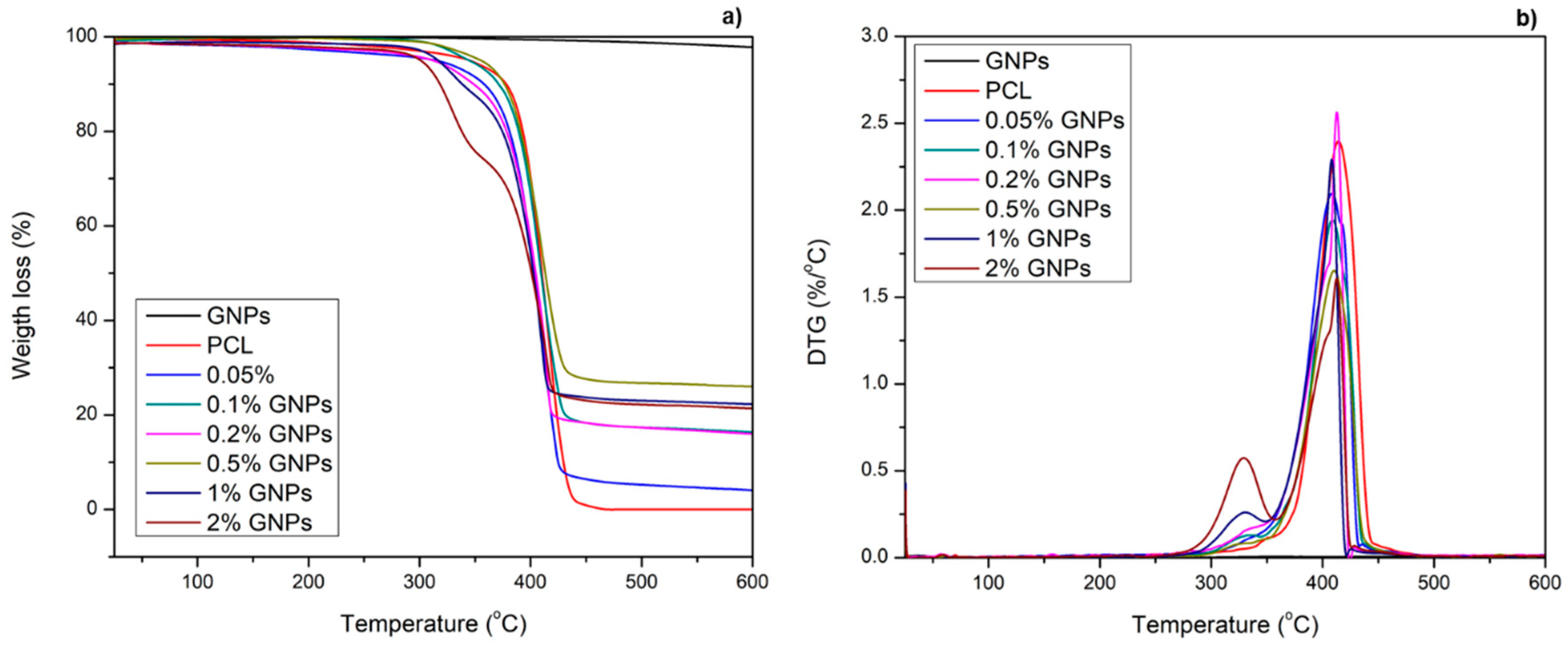
3.2. Thermal Analysis

The thermal decomposition behavior of the PCL microfibers, containing different GNPs concentrations, was evaluated by TGA. For this analysis, the samples were subjected to a controlled temperature increment up to 600 °C (Figure 7).

The TGA curves of the PCL and GNPs-PCL microfibers with different GNPs concentrations (Figure 7a) showed that there was one main loss step common to all samples, between approximately 350 °C and 450 °C, corresponding to the PCL degradation, as expected [39]. With the increasing concentration of GNPs, especially for the 1% and 2%, another loss step appeared between 250 °C and 350 °C, which was probably due to the loss of the acidic functional groups and residues of the exfoliation process [40,41,42]. DTG (Derivative Thermogravimetry) analysis (Figure 7b) demonstrated that the samples did not present a linear thermal behavior in relation to the percentage of GNPs. The maximum degradation peak of PCL was practically the same, at approximately 409 °C for all samples except one. The incorporation of 2% of GNPs promoted a shift of the peak to higher temperatures, from 409 °C (neat PCL sample) to 415 °C, which corresponded to an increase of 8 °C. Therefore, these results showed that although the thermal behavior was not linear, the tendency was to improve the thermal stability of the PCL membranes with the increase of GNPs concentration [39].

TGA can also be used as a quantitative analysis, providing information about the amount of the GNPs present in the developed samples. Taking into consideration all the weight losses and giving special attention to the residue percentage at the end of the heating process, the quantity of GNPs was calculated, using the Equation System (2). The sample of only PCL presented 1.80 wt% of residues, and the samples 0.05%GNPs-PCL, 0.1%GNPs-PCL, 0.2%GNPs-PCL, 0.5%GNPs-PCL, 1%GNPs-PCL, and 2%GNPs-PCL presented 8.45 wt%, 17.66 wt%, 20.05 wt%, 27.39 wt%, 24.70 wt%, and 24.76 wt% of total residues, respectively. Assuming that the samples were composed by only PCL and GNPs, the final GNPs percentage present on the samples after the impregnation was of 6.65 wt%, 15.86 wt%, 18.25 wt%, 25.59 wt%, 22.90 wt%, and 22.96 wt% for the samples 0.05%GNPs-PCL, 0.1%GNPs-PCL, 0.2%GNPs-PCL, 0.5%GNPs-PCL, 1%GNPs-PCL and 2%GNPs-PCL, respectively.

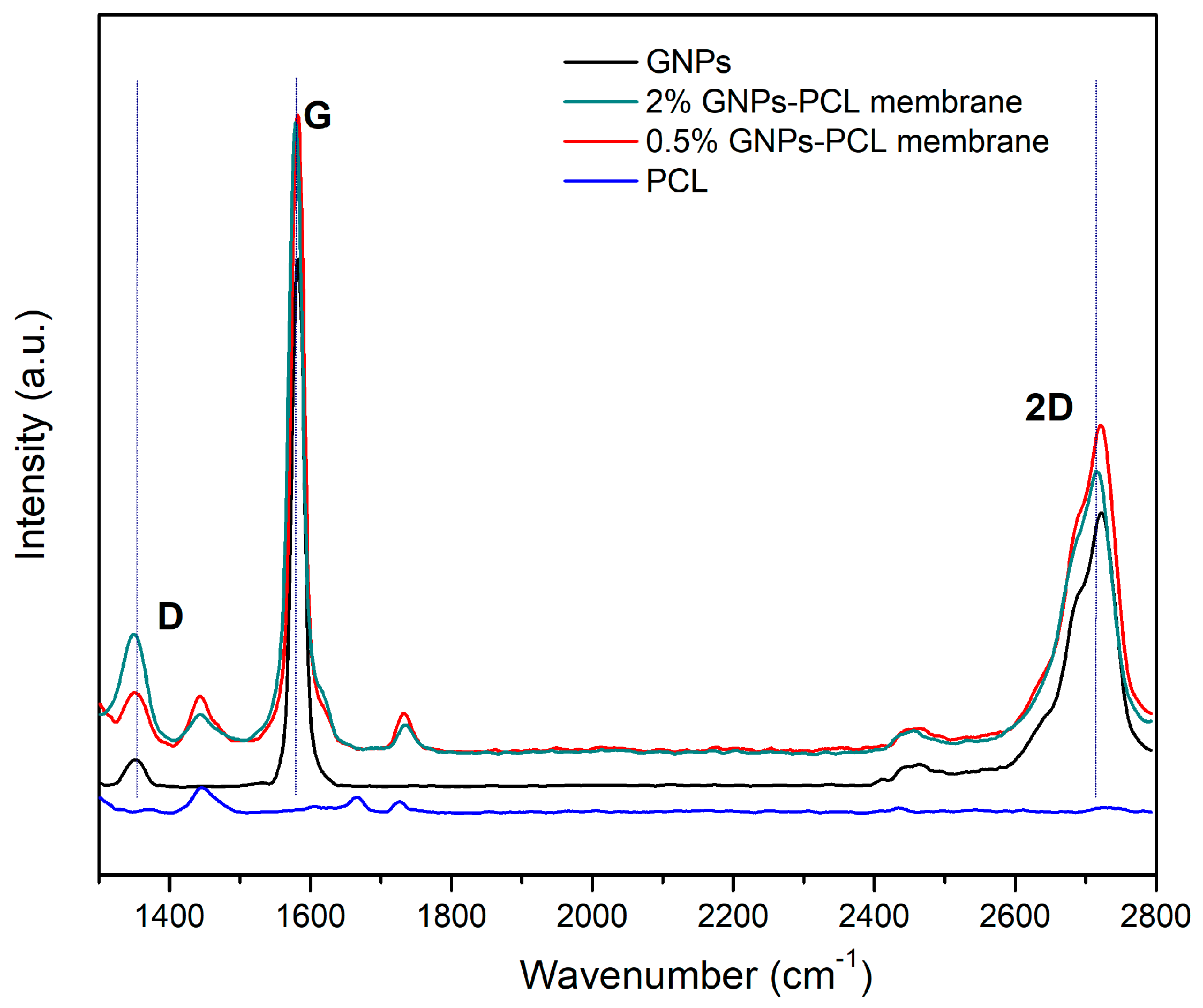
3.3. Raman Spectroscopy

Raman spectroscopy is one of the most commonly used characterization techniques for carbon-based materials. This technique can be efficiently used to monitor the number of layers, quality, doping level, and confinement of the materials [43]. In this work, Raman spectroscopy was employed in order to study the structure of the GNPs used and to verify their presence in the samples produced (Figure 8).

The presence of three characteristic peaks of graphitic structures can be observed in the spectrum of the GNPs and GNPs-PCL membranes (0.5% and 2%), corresponding to bands D, G, and 2D. The D and G bands are presented in all poly-aromatic hydrocarbons. The G peak is related to the stretching bond of all pairs of sp² atoms in both rings and chains. The D peak is due to the breathing modes of sp² atoms in rings [43]. The 2D band is representative of graphite and allows us to obtain information regarding the number of sheets that constituted the GNPs. This information can also be determined through the I2D/IG calculation. The D band represents the degree of defects present in the structure. Then, through the characteristic Raman peak intensity ratio ID/IG, it is possible to obtain qualitative and quantitative information regarding the structure, size and defects of the carbon-based materials [44].

The spectrum of the GNPs powder shows the D band peaking at approximately 1350 cm⁻¹. Compared with the G band, the D band presents a relatively low intensity with an ID/IG ratio of 0.08, indicating that these GNPs possessed few structural defects. Regarding the G band with higher intensity, it peaked at 1580 cm⁻¹. The 2D band peaked at ~2720 cm⁻¹, showing a lower intensity than the G band (I2D/IG = 0.52). This indicates that the GNPs were composed of graphene multilayers, as can also be observed in the amplified FESEM images in Figure 6d,f. As observed in Figure 8, regardless of the concentration of GNPs arranged in the membranes, the peaks for the D, G, and 2D bands are positioned in the same wavenumber as the GNPs powder. Besides this information, comparing the PCL membrane spectrum with the GNPs-PCL, it can be concluded that the GNPs were correctly incorporated onto the surface membranes.

3.4. Functional Properties Evaluation

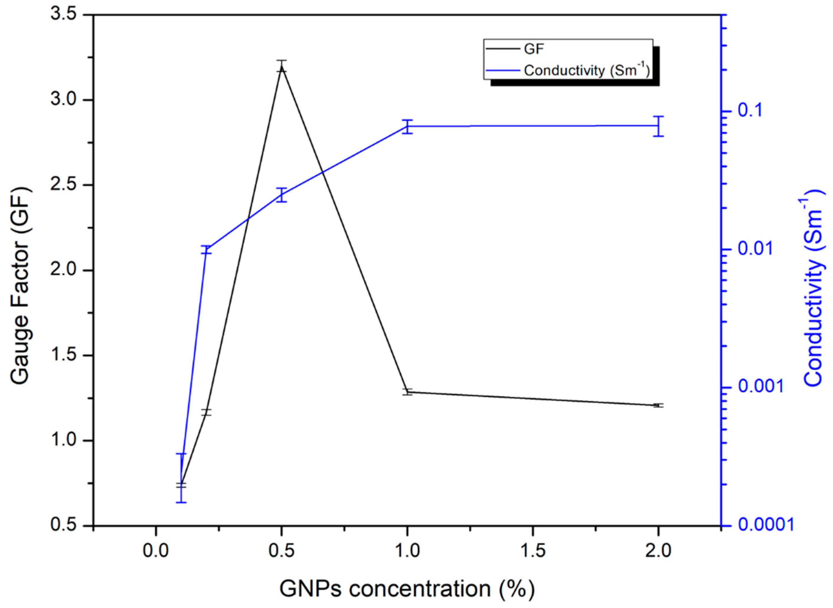
3.4.1. Electrical Conductivity

The electrical properties depend on several factors, such as the GNPs concentration, dispersion, homogeneity, agglomeration, and formation of conductive networks [45]. A thorough study of the influence of various aspects on the electrical properties of the developed samples was performed.

First, a comparison between the variation of the electrical resistance (Ω) and the concentration of GNPs present in the samples was performed, as illustrated in Figure 9.

It was possible to observe that the electrical resistance continuously decreased in response to the increasing GNPs concentration, as expected. The obtained results were 2.5 MΩ for 0.1%GNPs-PCL, 62.5 kΩ for 0.2%GNPs-PCL, 23.6 kΩ for 0.5%GNPs-PCL, 7.7 kΩ for 1%GNPs-PCL, and 7.5 kΩ for the 2%GNPs-PCL. Remembering that the electrical conductivity is the inverse of the resistivity, the electrical conductivity had an increase directly proportional to the GNPs concentration (Figure 9a). This behavior can be attributed to the increasing GNPs, which were mass impregnated onto the membranes, and the consequent network increment. The relationship between the duration of the impregnation process and its influence on the uploaded GNPs mass on the samples, and consequently, on the electrical resistance, was also studied. Regarding this, the uploaded GNPs mass also increased with increasing impregnation time, as expected (Figure 9b), which indicates that more GNPs were embedded into the PCL membranes with time. As a result, membranes with better electrical properties were obtained with higher impregnation times.

After studying the influence of the impregnation times on the electrical properties of the samples, the influence of the GNPs quantity, as well as the influence of the treatment of five successive washes and dryings on the electrical conductivity of the developed samples, was evaluated, measuring the electrical resistance on different places of the samples. The electrical conductivity values, calculated as described previously using the two-wire method, are shown in

Table 2. Electrical conductivity results as a function of the concentration of GNPs and the amount of water treatment cycles performed from 1 to 5.

Electrical Conductivity (S/m)
Sample	Water Treatment Cycle (0)	Water Treatment Cycle (1)	Water Treatment Cycle (2)	Water Treatment Cycle (3)	Water Treatment Cycle (4)	Water Treatment Cycle (5)
0.05%GNPs-PCL	6.00 × 10−9	6.67 × 10−9	6.15 × 10−9	1.00 × 10−8	1.06 × 10−8	6.43 × 10−9
0.1%GNPs-PCL	5.75 × 10−2	1.17 × 10−2	1.05 × 10−2	3.75 × 10−4	1.85 × 10−4	2.40 × 10−4
0.2%GNPs-PCL	0.29	0.24	0.21	0.02	0.01	0.010
0.5%GNPs-PCL	1.61	0.21	0.09	0.03	0.03	0.025
1%GNPs-PCL	3.01	0.56	0.43	0.19	0.13	0.078
2%GNPs-PCL	3.17	0.68	0.74	0.25	0.11	0.08

after each water treatment cycle and for the different GNPs concentrations.

As can be verified in the results shown in Table 2, as the presence of GNPs in the samples increased (higher concentration), the electrical conductivity also increased considerably, corroborating the well-known electrical properties of these particles [6].

The conductivity performance was also studied after each successive washing and drying cycle. In this sense, it can be observed that the electrical conductivity decreased as the number of washes increased. This was expected, since during the treatment, some of the GNPs present on the sample’s surface were released. However, these processes were essential in order to get rid of the excess of GNPs after the impregnation. For the sample produced with 0.05% of GNPs, the values of electrical conductivity were very low (6.43 × 10⁻⁹ S/m) at the end of the whole process. However, with 2%, the electrical conductivity value reached 0.08 S/m after the same number of cycles. Therefore, with higher quantities of GNPs on the samples, higher values of electrical conductivity were obtained, even after successive water treatment cycles. This phenomenon can be explained by the fact that GNPs concentration increases as the distance between the nanoparticles decreases, leading to a fluid movement of the electrons, forming larger electron clouds, and, as a consequence, decreasing the resistance of the material [20].

3.4.2. Piezoresistive Behavior

In line with the main objective of this work, a flexible sensor based on microfibers with a piezoresistive behavior was developed, the electrical response under mechanical stimuli of the samples was studied. For this, mechanical cyclic compressions were performed according to the methodology described before. The strain over a GNPs system results in a change of its global electronic properties [17]. When a material that has certain electrical characteristics is subjected to mechanical compression in a specific area, the difference between the internal and external pressure outside the studied area causes a bending in one part and, therefore, a bulge in another section of the membrane. This bulge will generate a pseudo-magnetic field, consequently decreasing the electrical resistance, which means that the electrons will be scattered by the compressed region. This behavior is reflected and quantified by the GF values for piezoresistive materials [6]

All the piezoresistive behavior tests were performed after the successive washing and drying treatments, with the objective to ensure the highest stability as possible in the results. In addition, 50 consecutive compression cycles were carried out, considering only the last 10 measurements in order to ensure the correct material relaxation and thus obtain the most reliable results possible.

The pressure applied on the samples induced their damage due to their very low thickness. The electrodes came into contact, making a short-circuit and resulting in unrealistic electrical resistance values. For this reason, a superposition of layers of the same membrane was carried out in order to obtain a suitable thickness for the test. The piezoresistive response obtained for the samples developed in this work are presented on Figure 10.

The neat PCL sample did not show any change in electrical resistance under mechanical compression, which confirms that this sample did not present piezoresistive behavior (Figure 10a). Since the development of piezoresistive sensors requires a conductive surface, this result was expected, considering that PCL does not have any electrical conductivity property per se. The same behavior occurred for 0.05%GNPs-PCL (Figure 10b) sample as well, demonstrating that the GNPs present onto the sample were not enough to obtain electrical conductivity nor a piezo resistivity response. However, using 0.1%, 0.2%, 0.5%, 1%, and 2% of GNPs (Figure 10c–g, respectively), it is possible to observe a change in the electrical resistance under mechanical deformation, demonstrating the piezoresistive behavior of these samples. Moreover, a linearity in the variation of the electrical resistance was observed for all the strain/release cycles. In addition, the sample with 0.5% GNPs was the one to demonstrate higher variation in the electrical resistance with the applied strain. The sensitivity of the sensors can be expressed by the GF. The GF values were calculated using Equation (6). These results are presented on

Table 3. Average Gauge Factor (GF) values obtained for each sample.

Sample	GF	Error
0.1%GNPs-PCL	0.74	0.01
0.2%GNPs-PCL	1.17	0.02
0.5%GNPs-PCL	3.20	0.03
1%GNPs-PCL	1.29	0.02
2%GNPs-PCL	1.21	0.01

and were calculated as the average of 10 ascending and descending cycles.

The highest obtained GF value (3.20) was observed for the sample with 0.5% of GNPs, being that an increase of the GF values between 0.1% and 0.5% was verified. The finding shows that this concentration of GNPs (0.5%) resulted in the higher sensitivity to mechanical deformation, which is related with greater variations in the electrical resistance, as confirmed by the Figure 10e. Hence, the 0.5%GNPs-PCL sample is the most promising to be used as a piezoresistive sensor. Above the 0.5% concentration, the GF values decreased, reaching 1.21 for the 2%GNPS-PCL sample. Moreover, Figure 11 shows the relation between the measured electrical conductivity and the calculated GF for each GNPs-PCL sample as a function of the GNPs concentration. For GNPs percentages between 0.1% and 0.5%, there was an increase for both electrical conductivity and GF. Between 0.5% and 2%, the trend of the GF decreased while the electrical conductivity continued to increase (Figure 11).

In literature, the theory for piezoresistive materials regarding the percolation threshold is presented as the limit where the electrical conductivity of materials varies in several orders of magnitude (within this range) and where there is very little variation in conductivity before and after that limit, with a tendency to stabilize it after that point. In this way, in this threshold, the maximum conductivity achieved can be obtained for an optimal piezoresistive behavior (higher GF values) [6]. In this specific case, it was confirmed that the sample with 0.5% of GNPs presents the best performance near the percolation threshold (Figure 11).

4. Conclusions

The main goal of this work was to develop a piezoresistive material to use as a flexible pressure sensor based on the incorporation of GNPs onto PCL electrospun membranes. The proposed material seems to be very promising for the realization of pressure sensors in a broad range of applications, especially applications where the sensor’s flexibility and light weight is of great importance, such as in military equipment. FESEM and Raman Spectroscopy validated the presence of GNPs onto the microfibers’ structures, confirming their correct adhesion to the membranes. Moreover, their successful incorporation by the post-impregnation method was also visible not only by the FESEM images, but also by the measurement of the L* (lightness) parameter, proving that a homogeneous distribution of the GNPs all over the microfibers’ surfaces was obtained. TGA analysis gave information about the thermal behavior of the developed samples, as well as the influence of the GNPs on the degradation temperatures. For the sample with 2% of GNPs, an increase of 8 °C for the maximum degradation temperature of PCL was observed when compared to the neat PCL sample, demonstrating that the maximum GNPs concentration used improved this property. Raman spectroscopy allowed the study of the GNPs structure, proving that the GNPs used in this work presented few structural defects and were composed by graphene multilayers.

Further, electrical properties such as conductivity and piezoresistive performance were studied. With the increase of GNPs present on the surface of the fibers, the distance between the nanoparticles decreased, forming larger electron clouds. Consequently, the electrical resistance decreased. A maximum electrical conductivity value of 0.08 S/m was obtained for the 2%GNPs-PCL sample after five successive water/drying cycles. The samples with 0.1%, 0.2%, 0.5%, 1%, and 2% of GNPs were able to change their electrical resistance under external pressures and presented excellent durability and reversibility to repetitive compression, demonstrating their piezoresistive behavior over the cycles. The best values of GF (3.20) were obtained for the membranes with 0.5% of GNPs. The high sensitivity makes it interesting for wearable health care systems. In combination with the light weight and flexibility of the developed systems, an effective, comfortable, and adaptable sensor can be obtained.

In summary, a simple and cost-effective method for the development of a very flexible piezoresistive sensor based on conductive biodegradable electrospun microfibers was proposed. This work may not only provide an electrospinning and GNPs-based approach for the building of flexible piezoresistive sensors, but also an alternative that can be used for the development of a wearable sensor, with great potential in monitoring of human motions and vital signs for soldiers’ equipment applications. The developed sensors bring a novel alternative for this type of application, since they are flexible and adaptable, with a constant behavior during consecutive compression cycles. The sensors also present a high sensitivity, being highly effective without compromising the comfort and weight of the user. This work also presents a strategy for the obtention of homogenous electrospun fibers functionalized with GNPs, which are known for their agglomeration problems.

References

1. Ferreira, D.P.; Costa, S.M.; Felgueiras, H.P.; Fangueiro, R. Smart and Sustainable Materials for Military Applications Based on Natural Fibres and Silver Nanoparticles. Key Eng. Mater. 2019, 812, 66–74. [Google Scholar] [CrossRef]
2. Costa, J.C.; Spina, F.; Lugoda, P.; Garcia-Garcia, L.; Roggen, D.; Münzenrieder, N. Flexible Sensors—From Materials to Applications. Technologies 2019, 7, 35. [Google Scholar] [CrossRef] [Green Version]
3. Shi, H.; Zhao, H.; Liu, Y.; Gao, W.; Dou, S.C. Systematic analysis of a military wearable device based on a multi-level fusion framework: Research directions. Sensors 2019, 19, 2651. [Google Scholar] [CrossRef] [PubMed] [Green Version]
4. Costa, S.M.; Ferreira, D.P.; Ferreira, A.; Vaz, F.; Fangueiro, R. Multifunctional Flax Fibres Based on the Combined Effect of Silver and Zinc Oxide (Ag/ZnO) Nanostructures. Nanomaterials 2018, 8, 1069. [Google Scholar] [CrossRef] [PubMed] [Green Version]
5. Zeng, W.; Shu, L.; Li, Q.; Chen, S.; Wang, F.; Tao, X.-M. Fiber-Based Wearable Electronics: A Review of Materials, Fabrication, Devices, and Applications. Adv. Mater. 2014, 26, 5310–5336. [Google Scholar] [CrossRef]
6. Pereira, P.; Ferreira, D.P.; Araújo, J.C.; Ferreira, A.; Fangueiro, R. The Potential of Graphene Nanoplatelets in the Development of Smart and Multifunctional Ecocomposites. Polymers 2020, 12, 2189. [Google Scholar] [CrossRef]
7. Araújo, J.C.; Ferreira, D.P.; Teixeira, P.; Fangueiro, R. In-Situ synthesis of CaO and SiO2 nanoparticles onto jute fabrics: Exploring the multifunctionality. Cellulose 2020. [Google Scholar] [CrossRef]
8. Muñoz, V.; Buffa, F.; Molinari, F.; Hermida, L.G.; García, J.J.; Abraham, G.A. Electrospun ethylcellulose-based nanofibrous mats with insect-repellent activity. Mater. Lett. 2019, 253, 289–292. [Google Scholar] [CrossRef]
9. Ojha, S. Structure-Property Relationship of Electrospun Fibers. In Electrospun Nanofibers; Elsevier Ltd.: Amsterdam, The Netherlands, 2017; ISBN 9780081009116. [Google Scholar]
10. Wang, X.; Zhao, H.; Turng, L.S.; Li, Q. Crystalline morphology of electrospun poly(ε-caprolactone) (PCL) nanofibers. Ind. Eng. Chem. Res. 2013, 52, 4939–4949. [Google Scholar] [CrossRef]
11. Mochane, M.J.; Motsoeneng, T.S.; Sadiku, E.R.; Mokhena, T.C.; Sefadi, J.S. Morphology and properties of electrospun PCL and its composites for medical applications: A mini review. Appl. Sci. 2019, 9, 2205. [Google Scholar] [CrossRef] [Green Version]
12. Yew, C.H.T.; Azari, P.; Choi, J.R.; Muhamad, F.; Pingguan-Murphy, B. Electrospun polycaprolactone nanofibers as a reaction membrane for lateral flow assay. Polymers 2018, 10, 1387. [Google Scholar] [CrossRef] [PubMed] [Green Version]
13. Zhu, J.; Jasper, S.; Zhang, X. Chemical Characterization of Electrospun Nanofibers. In Electrospun Nanofibers; Elsevier Ltd.: Amsterdam, The Netherlands, 2017; ISBN 9780081009116. [Google Scholar]
14. Bhardwaj, N.; Kundu, S.C. Electrospinning: A fascinating fiber fabrication technique. Biotechnol. Adv. 2010, 28, 325–347. [Google Scholar] [CrossRef] [PubMed]
15. Zhao, Z.; Li, B.; Xu, L.; Qiao, Y.; Wang, F.; Xia, Q.; Lu, Z. A sandwich-structured piezoresistive sensor with electrospun nanofiber mats as supporting, sensing, and packaging layers. Polymers 2018, 10, 575. [Google Scholar] [CrossRef] [PubMed] [Green Version]
16. Fiorillo, A.S.; Critello, C.D.; Pullano, A.S. Theory, technology and applications of piezoresistive sensors: A review. Sensors Actuators A Phys. 2018, 281, 156–175. [Google Scholar] [CrossRef]
17. Flynn, G. Atomic Scale Imaging of the Electronic Structure and Chemistry of Graphene and its Precursors on Metal Surfaces. Final Tech. Rep. Submitt. Dep. Energy 2014, 1, 1–13. [Google Scholar]
18. Cataldi, P.; Athanassiou, A.; Bayer, I.S. Graphene Nanoplatelets-Based Advanced Materials and Recent Progress in Sustainable Applications. Appl. Sci. 2018, 8, 1438. [Google Scholar] [CrossRef] [Green Version]
19. Bahiraei, M.; Heshmatian, S. Graphene family nanofluids: A critical review and future research directions. Energy Convers. Manag. 2019, 196, 1222–1256. [Google Scholar] [CrossRef]
20. Milovanović, S.P.; Peeters, F.M. Strained graphene structures: From valleytronics to pressure sensing. NATO Sci. Peace Secur. Ser. A Chem. Biol. 2018, 3–17. [Google Scholar] [CrossRef] [Green Version]
21. Baloda, S.; Ansari, Z.A.; Singh, S.; Gupta, N. Development and Analysis of Graphene Nanoplatelets (GNP) Based Flexible Strain Sensor for Health Monitoring Applications. IEEE Sens. J. 2020. [Google Scholar] [CrossRef]
22. Sabzi, M.; Jiang, L.; Liu, F.; Ghasemi, I.; Atai, M. Graphene nanoplatelets as poly(lactic acid) modifier: Linear rheological behavior and electrical conductivity. J. Mater. Chem. A 2013, 1, 8253–8261. [Google Scholar] [CrossRef]
23. Lu, S.; Tian, C.; Wang, X.; Zhang, L.; Du, K.; Ma, K.; Xu, T. Strain sensing behaviors of GnPs/epoxy sensor and health monitoring for composite materials under monotonic tensile and cyclic deformation. Compos. Sci. Technol. 2018, 158, 94–100. [Google Scholar] [CrossRef]
24. Moriche, R.; Jiménez-Suárez, A.; Sánchez, M.; Prolongo, S.G.; Ureña, A. High sensitive damage sensors based on the use of functionalized graphene nanoplatelets coated fabrics as reinforcement in multiscale composite materials. Compos. Part B Eng. 2018, 149, 31–37. [Google Scholar] [CrossRef]
25. Souri, H.; Bhattacharyya, D. Wearable strain sensors based on electrically conductive natural fiber yarns. Mater. Des. 2018, 154, 217–227. [Google Scholar] [CrossRef]
26. Sagitha, P.; Reshmi, C.R.; Sundaran, S.P.; Sujith, A. Recent advances in post-modification strategies of polymeric electrospun membranes. Eur. Polym. J. 2018, 105, 227–249. [Google Scholar] [CrossRef]
27. Ekram, B.; Abdel-Hady, B.M.; El-Kady, A.M.; Amr, S.M.; Waley, A.I.; Guirguis, O.W. Optimum parameters for the production of nano-scale electrospun polycaprolactone to be used as a biomedical material. Adv. Nat. Sci. Nanosci. Nanotechnol. 2017, 8. [Google Scholar] [CrossRef] [Green Version]
28. Guarino, V.; Gentile, G.; Sorrentino, L.; Ambrosio, L. Polycaprolactone: Synthesis, Properties, and Applications. In Encyclopedia of Polymer Science and Technology, 4th ed.; Mark, H., Ed.; John Wiley & Sons: New Jersey, NJ, USA, 2017; ISBN 0471440264. [Google Scholar]
29. Safarova, V.; Gregr, J. Electrical Conductivity Measurement of Fibers and Yarns. In Proceedings of the 7th International Conference, TEXSCI, Liberec, Czech Republic, 6–8 September 2010; pp. 2–9. [Google Scholar]
30. Singh, Y. Electrical Resistivity Measurements: A Review. Int. J. Mod. Phys. Conf. Ser. 2013, 22, 745–756. [Google Scholar] [CrossRef]
31. Fotheringham, S.; Wgener, M.; Longley, P.; Goodchild, M.; Maguire, D. Lecture 9: Piezoresistivity. Univ. Victoria Dept Mech. Eng. 2019, 466, 1–13. [Google Scholar]
32. Mondal, S. Review on Nanocellulose Polymer Nanocomposites. Polym. Plast. Technol. Eng. 2018, 57, 1377–1391. [Google Scholar] [CrossRef]
33. Rong, D.; Chen, P.; Yang, Y.; Li, Q.; Wan, W.; Fang, X.; Zhang, J.; Han, Z.; Tian, J.; Ouyang, J. Fabrication of Gelatin/PCL Electrospun Fiber Mat with Bone Powder and the Study of Its Biocompatibility. J. Funct. Biomater. 2016, 7, 6. [Google Scholar] [CrossRef]
34. Bellani, C.F.; Pollet, E.; Hebraud, A.; Pereira, F.V.; Schlatter, G.; Avérous, L.; Bretas, R.E.S.; Branciforti, M.C. Morphological, thermal, and mechanical properties of poly(ε-caprolactone)/poly(ε-caprolactone)-grafted-cellulose nanocrystals mats produced by electrospinning. J. Appl. Polym. Sci. 2016, 133, 4–11. [Google Scholar] [CrossRef]
35. Croisier, F.; Duwez, A.S.; Jérôme, C.; Léonard, A.F.; Van Der Werf, K.O.; Dijkstra, P.J.; Bennink, M.L. Mechanical testing of electrospun PCL fibers. Acta Biomater. 2012, 8, 218–224. [Google Scholar] [CrossRef] [PubMed]
36. Roso, M.; Sundarrajan, S.; Pliszka, D.; Ramakrishna, S.; Modesti, M. Multifunctional membranes based on spinning technologies: The synergy of nanofibers and nanoparticles. Nanotechnology 2008, 19. [Google Scholar] [CrossRef] [PubMed]
37. Metwally, S.; Ferraris, S.; Spriano, S.; Krysiak, Z.J.; Kaniuk, Ł.; Marzec, M.M.; Kim, S.K.; Szewczyk, P.K.; Gruszczyński, A.; Wytrwal-Sarna, M.; et al. Surface potential and roughness controlled cell adhesion and collagen formation in electrospun PCL fibers for bone regeneration. Mater. Des. 2020, 194. [Google Scholar] [CrossRef]
38. Wang, B.; Li, H.; Li, L.; Chen, P.; Wang, Z.; Gu, Q. Electrostatic adsorption method for preparing electrically conducting ultrahigh molecular weight polyethylene/graphene nanosheets composites with a segregated network. Compos. Sci. Technol. 2013, 89, 180–185. [Google Scholar] [CrossRef]
39. Vogel, C.; Siesler, H.W. Thermal degradation of poly(ε-caprolactone), poly(L-lactic acid) and their blends with poly(3-hydroxy-butyrate) studied by TGA/FT-IR spectroscopy. Macromol. Symp. 2008, 265, 183–194. [Google Scholar] [CrossRef]
40. Gao, R.; Hu, N.; Yang, Z.; Zhu, Q.; Chai, J.; Su, Y.; Zhang, L.; Zhang, Y. Paper-like graphene-Ag composite films with enhanced mechanical and electrical properties. Nanoscale Res. Lett. 2013, 8, 32. [Google Scholar] [CrossRef] [Green Version]
41. Kumar, R.; Kumar, M.; Kumar, A.; Singh, R.; Kashyap, R.; Rani, S.; Kumar, D. Surface modification of Graphene Oxide using Esterification. Mater. Today Proc. 2019, 18, 1556–1561. [Google Scholar] [CrossRef]
42. Hu, N.; Gao, R.; Wang, Y.; Wang, Y.; Chai, J.; Yang, Z.; Kong, E.S.-W.; Zhang, Y. The preparation and characterization of non-covalently functionalized graphene. J. Nanosci. Nanotechnol. 2012, 12, 99–104. [Google Scholar] [CrossRef] [Green Version]
43. Ferrari, A.C. Raman spectroscopy of graphene and graphite: Disorder, electron-phonon coupling, doping and nonadiabatic effects. Solid State Commun. 2007, 143, 47–57. [Google Scholar] [CrossRef]
44. Munir, K.S.; Qian, M.; Li, Y.; Oldfield, D.T.; Kingshott, P.; Zhu, D.M.; Wen, C. Quantitative Analyses of MWCNT-Ti Powder Mixtures using Raman Spectroscopy: The Influence of Milling Parameters on Nanostructural Evolution. Adv. Eng. Mater. 2015, 17, 1660–1669. [Google Scholar] [CrossRef]
45. Sadasivuni, K.K.; Ponnamma, D.; Kim, J.; Thomas, S. Electrical Properties of Graphene Polymer Nanocomposites. In Graphene-Based Polymer Nanocomposites in Electronics; Springer: Cham, Switzerland, 2015; pp. 25–47. [Google Scholar] [CrossRef]
Figure 1. Schematic flow chart of the graphene nanoplatelets (GNPs)- polycaprolactone (PCL) membranes preparation.
Applsci 11 01124 g001
Figure 2. Schematic representation of the experimental configuration for the piezoresistive performance evaluation.
Applsci 11 01124 g002
Figure 3. Field Emission Scanning Electron Microscopy (FESEM) images of the electrospun fibers produced using different PCL concentrations and their diameter distribution histograms: (a) 15%; (b) 20%; (c) 25% (w/v) in Chloroform (CHF)/Dimethylformamide (DMF) (4:1). From left to right: 2000× (50 µm); 10,000× (10 µm).
Applsci 11 01124 g003
Figure 4. FESEM images of the electrospun PCL fibers and their diameter distribution histograms produced with different process conditions (applied voltage, flow rate, and needle-collector distance: (a) 25 kV, 240 mm, 1 mL/h; (b) 25 kV, 240 mm, 2 mL/h; (c) 28 kV, 240 mm, 1 mL/h; (d) 28 kV, 240 mm, 2 mL/h; (e) 25 kV, 260 mm, 1 mL/h; (f) 25 kV, 260 mm, 2 mL/h; (g) 28 kV, 260 mm, 1 mL/h; (h) 28 kV, 260 mm, 2 mL/h, to a PCL concentration of 15% (w/v) in CHF/DMF (4:1).
Applsci 11 01124 g004aApplsci 11 01124 g004bApplsci 11 01124 g004c
Figure 5. Schematic illustration of the dipping method for GNPs-PCL membranes preparation. The PCL membranes were immersed in an GNPs/Ethanol solution at room temperature for 1 h. Finally, the coated membranes were dried at room temperature.
Applsci 11 01124 g005
Figure 6. FESEM images of (a) and (b) PCL microfibers; (c) and (d) 0.2%GNPs-PCL membranes; (e) and (f) 2%GNPs-PCL membranes. The magnifications used for these images was of 10,000× (10 μm) and 50,000× (2 μm), from the left to the right.
Applsci 11 01124 g006
Figure 7. Thermogravimetric Analysis (TGA) (a) and Derivative Thermogravimetry (DTG) (b) curves of GNPs, PCL, and GNPs-PCL membranes with different percentages of GNPs.
Applsci 11 01124 g007
Figure 8. Raman spectra of the GNPs (black) PCL membrane (dark blue), 0.5% (red), and 2%GNPs-PCL membrane (light blue).
Applsci 11 01124 g008
Figure 9. Electrical properties of the samples: (a) Resistance and uploaded GNPs mass of the GNPs-PCL membranes with an immersion of 1 h and after five consecutive washing/drying treatments; (b) Resistance and uploaded GNP mass for 1%GNPs-PCL membrane for several impregnation times (5 min, 15 min, 30 min, and 60 min).
Applsci 11 01124 g009
Figure 10. Piezoresistive response of PCL membrane (a), 0.05%GNPs-PCL membrane (b), 0.1%GNPs-PCL membrane (c), 0.2%GNPs-PCL membrane (d), 0.5%GNPs-PCL membrane (e), 1%GNPs-PCL membrane (f), and 2%GNPs-PCL membrane (g).
Applsci 11 01124 g010
Figure 11. Electrical conductivity and GF in relation to the GNPs concentration.
Applsci 11 01124 g011