Featured Application
The simulation method in this article is proposed to gain the sound field in the cavity of a rotating automobile tire. And the test about sound pressure is performed to validate the simulation method.
Abstract
As we all know, the tire acoustic cavity resonance noise (TACRN) can cause irritating noise in a vehicle, but it is evidently difficult to be weakened. To obtain accurately the characteristics of TACRN is a key step of attenuating TACRN. In this paper, a simulation method, in which a simplified finite element model of automobile tire with acoustic cavity introducing the rotation of automobile tire is established, is proposed to gain the sound field in the cavity of a rotating automobile tire. And the test of sound pressure in a rotating tire is also performed to validate the proposed simulation method. The comparisons between the simulation and experimental consequences show a satisfying conclusion. Furthermore, the influence factors of the rotating speed, the inflation pressure of the tire and the load on the sound field of automobile tire acoustic cavity are calculated and analyzed.
1. Introduction
As we all know, the tire acoustic cavity resonance noise (TACRN) can cause irritating noise in a vehicle. When a car is running, the interaction between road surface with certain roughness and tire tread with certain pattern will produce the excitation which frequency bandwidth is wide, thus resulting in TACRN. In the range of 200–260 Hz, the contribution of TACRN is most significant [1,2,3,4,5,6,7,8].
To fully understand the characteristics of TACRN is a key step of attenuating TACRN. To this aim, many researchers have performed a series of investigations, especially in building tire simulation models with acoustical cavities and the influences of load and velocity on TACRN. Sakata et al. [9] first clarified the effects of automobile tire acoustic cavity resonance by a simulation approach and by road tests, and the consequences evidently indicated that the major peak was at the first mode of automobile tire cavity resonance in the circumferential direction. In order to understand the frequency characteristics of TACRN, Thompson [10] developed a closed form solution to forecast the tire cavity resonance frequencies of the deflected tire and performed experimental verification, and it was also indicated that the cavity resonance of deflected tire generated forces acting at the chassis axle spindle simultaneously along vertical and fore-aft directions at slightly different frequencies.
Some researchers focused on the simulation analysis to understand TACRN. Mohamed and Wang et al. [11,12] paid attention to the influences of the coupling of tire, cavity and rim on the TACRN, and verified the simulation models by using different analysis approaches. It was found that the helium gas in place of the air inside the tire cavity was valid. Peng et al. [13] explored the mechanism of TACRN by using simulation and experimental methods. The analytical model revealed the critical mode inducing TACRN, and the numerical model revealed why the noise existed in two frequencies. At last, a countermeasure was provided to suppress TACRN. Since TACRN comes from the interaction between road and automobile tire, the road roughness should be introduced. Yi et al. [14] simulated the sound field of the automobile tire cavity because of the roughness of the road. Furthermore, some influence factors of automobile tire load and inflation pressure were also researched. The consequences showed that the inner sound pressure’s peak rose obviously when the inflation pressure increased and inner sound pressure’s peak increased slightly when the tire load went up.
Aiming at exploring the mechanism of TACRN by experiment, Tanaka et al. [15] used a multi-microphone system to measure the SPL and mode shapes of TACRN, and the test consequences indicated that SPL of the special tire with polyurethane foam was lower than that of the baseline tire. Feng et al. [16,17] proposed an analytical tire model, and presented test verifications of forecast on the peak frequency and the consequences showed that analytical tire model can be used to forecast TACRN for a rolling automobile tire in the early design stage. Hu et al. [18] performed the test and research of the sound pressure distribution in a rotating tire, and obtained the correlative characteristics of sound pressure in the tire. These achievements lay a good foundation to understand TACRN. In fact, the tire and inside air medium are rotating, so to understand the effect of the rotation on TACRN is very crucial to predict and weaken the TACRN, resulting in the reduced interior noise of a car. However up to now, there is no articles indicating how to simulate TACRN since for the simulation of the rotating tire cavity the flow-solid coupling and the convergence of the simulation calculation and the rotating effect need to be taken into account. However, the current simulation software has certain limitations in dealing with the rotating effect of the tire and cavity.
Aiming at these problems, the finite element model (FEM) of a tire coupling with the inside acoustic medium is established in terms of the real tire firstly. Then, the rotation of tire is introduced through the establishment of the equivalent model, and the cavity sound pressure distributions of a rotating tire are emulated. Besides, the test of sound field in a rotating tire is performed to validate the proposed simulation method. Furthermore, the influence factors of the tire rotational speed, the tire inflation pressure and the tire load on the sound field are analyzed. However, the influence of tire compound, the tread pattern, wear and usage time on noise is not considered, since the influence of these factors on tire acoustic cavity resonance noise is more complex and the simulation analysis is more difficult. These works are helpful to understand accurately the characteristics of TACRN.
2. Construction of FEM of a Rotating Tire
A tire of 185/60R15 is studied where the material properties are obtained from the tire manufacturer. Since the stiffness of the wheel is much greater than that of a tire, the automobile wheel is assumed as a rigid body in the simulation process. The tread pattern features are ignored while the cross-section characteristics of the tire are retained. Beside, a tire is very complex structure and it is formed by layers of parallel string reinforcements and rubber parts. In modeling of the tire, a two-dimensional (2D) FEM of automobile tire is built first, and then revolved into a three-dimensional (3D) FEM of automobile tire. The 2D FEM of tire with the size of 185/60R15 is built in Abaqus software, as show in Figure 1. In 3D FEM of tire, the sidewall, tread, apex, belt and bead are modeled according to the real automobile tire in Figure 2a. However, the inner liner is ignored because of its insignificant effect on TACRN. The acoustic medium (air) which fits the inner surface of the tire is modelled as displayed in Figure 2b, and there are a total of 97,440 elements in 3D FEM of tire. Considering that the large deformation of the tire and the non-linear contact behavior may occur in the simulation, the C3D8R and C3D6 elements are adopted to discretize the rubber parts, and the AC3D8R and AC3D6 elements are adopted to discretize the air part. The rubber is a typical nearly incompressible hyperelastic material, and the non-linear behavior of each rubber component in tire is described by Yeoh constitutive model. The hyperelastic properties of the rubber components determined from uniaxial test results are shown in Table 1 [19]. In the tire model, the component of tire bead is simplified as an isotropic structure with steel material property. The validation of acoustic-structural model is performed by the tire structural modal and acoustic modal experiment and shown in our previous researches [14,20,21]. Yi et al. [14] had simulated and tested the structural modal characteristics of the tire in inflated states and loaded states, and the simulation and test results showed that a good agreement and indicated the accuracy of the constructed model. Dong et al. [20,21] simulated the acoustic mode of tire cavity by sweep-frequency speed excitation, and the sweep-frequency speed excitation tests were performed in order to verify above simulation results as well as the validity of the FE model, and the simulation and test results showed that a good consistency. However, their research did not introduce the rotation of tire.
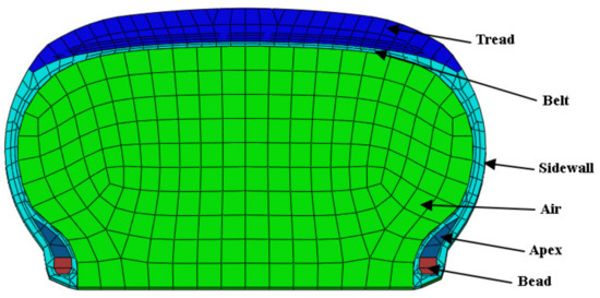
Figure 1.
2D FEM of tire.
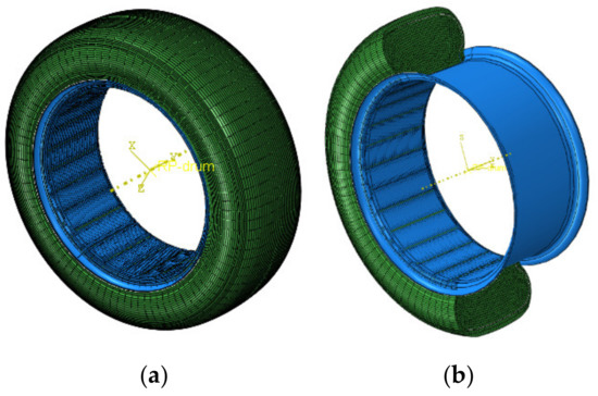
Figure 2.
Tire FEM: (a) 3D FEM of tire; (b) Tire model coupling with acoustic medium.

Table 1.
Rubber material parameters in tire.
According to the actual test equipment [18], a simplified but full scale three-dimensional drum model of the tire-test machine for TACRN is built in Abaqus software. The structural parameters of the finite element model are the same as those of the actual test tire with the test drum machine equipment. The wheel rim type is 5.5 J × 15, and the diameter of the drum is 1.7 m. The wheel rim and drum are presumed to be rigid bodies, as indicated in Figure 3. The boundary conditions are that the surface of tire contacts the surface of the drum in order to simulate the load, and the constraint type of tire and air is tie, and same for the constraint type of tire and wheel rim. In inflation and load analysis step, the DOFs of drum and tire-wheel assembly model are all limited, but in rotating analysis step, the rotation DOF around axis of the drum model is released. The compound, tread pattern, the wear, and the type of road are very important, these factors are not the research goal and core content of this paper, so these factors are not considered.
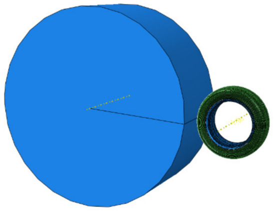
Figure 3.
FEM of a rotating tire and driving drum.
In the rolling tire test, the automobile tire is loaded against the roller drum through a hydraulic actuation system and a rail. The roller drum drives the tire-wheel assembly to rotate, so that the correlative load is able to be measured. Besides, the air in the cavity rotates clockwise with the tire-wheel assembly. In order to accurately simulate the effect of tire rotation on the TACRN, the tire needs to be driven to rotate. However, the simulation in the software cannot be performed because of the non-convergence of the simulation calculation arising from the acoustic mesh element of the air not rotating with the automobile tire.
In order to simulate the sound field of TACRN, some equivalent processes are required. For example, the acoustic element in the air cavity and tire-wheel assembly are assumed to be non-rotational, but the roller drum is assumed to rotate anticlockwise around the center axis of the spindle axle of the tire-wheel assembly to demonstrate the interaction between the tire and roller drum. The stimulation excitation in the simulation comes from the extrusion deformation and the fold bending between the roller drum and the tire.
To model the rotating tire coupled with inside acoustic medium and simulate the sound field of TACRN, three simulation steps are required and shown as follows. The first step is to fix the tire-wheel assembly and inflate the tire. The second step is to impose radial force to the surface of the tire by changing the contact displacement between the drum and the tire to simulate the load. Finally, the third step is that the drum rotates anticlockwise around the center axis of the spindle axle of the tire-wheel assembly, and the simulated rotation duration is set to be 2 s at a constant rotational speed. Figure 4 is a schematic diagram of simulated rotational tire, and the rotational roller drum in the anticlockwise direction around the center axis of the spindle axle of the tire-wheel assembly. In the experiment, the vehicle speeds are set as 40, 50 and 60 km/h respectively, while the rotational angular speeds of the roller drum are set as the equivalent ones and the tire remains to be stationary. This process can ensure the same contact relation between the tire and drum as the real experiment for setting the static tire and the static air acoustic element of tire cavity.
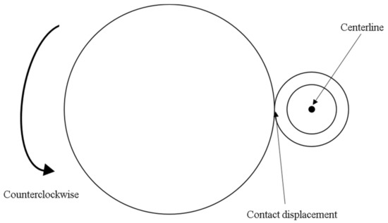
Figure 4.
Schematic diagram of simulated rotational tire.
The simulation is implemented by explicit algorithm in Abaqus. The operational conditions of the tire and drum are shown in Table 2. The angular speed of the roller drum corresponding to the vehicle speed is also shown in Table 2. The operational conditions in the simulation are the combination of different tire inflation pressures, vehicle speeds and loads in Table 2.
Table 2.
Different operational conditions of the tire and drum.
3. Simulation Analysis and Experimental Validation of Sound Pressure Distribution in the Acoustic Cavity of a Rotating Tire
In the experiment, the tire-wheel assembly is pushed to the drum of the tire-testing machine by a controllable oil cylinder through rail and is driven to revolve by the drum, so its angular velocity and the load on the tire can be determined. The wireless telemetering device collects the sound pressure signal in the tire acoustic cavity real-timely. For each experiment, the tire rotates clockwise, and the customized sound pressure sensor starts from the farthest away from the contact surface of the tire with the drum of the tire-testing machine. Ultimately, the sound pressure distributions in different conditions of the tire are obtained by changing the tire inflation pressure, the angular velocity and the load on the tire respectively. Figure 5a is a position diagram of the particular sensor that is attached to the internal face of the automobile tire.
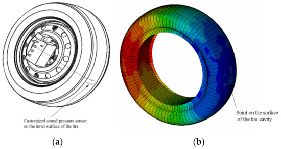
Figure 5.
Position of the sensor in the test and selected point on the tire cavity finite element model: (a) Position of the customized sensor; (b) Position of the selected point.
Taking the case of the tire rotational velocity equivalent to the vehicle speed of 60 km/h, the tire load of 4500 N and the inflation pressure of 2.2 bar as an example, the simulation is performed. Since the midpoints on the outer surface of the tire cavity which corresponding to the position of the customized sensor have similar time domain characteristics of sound pressure, any midpoint on the external surface of the tire FEM is selected, as shown in Figure 5b. The time-domain diagram of sound pressure at the midpoint on the outer face of the automobile tire cavity is shown in Figure 6a, and the frequency spectrum of its amplitude are displayed in Figure 6b.
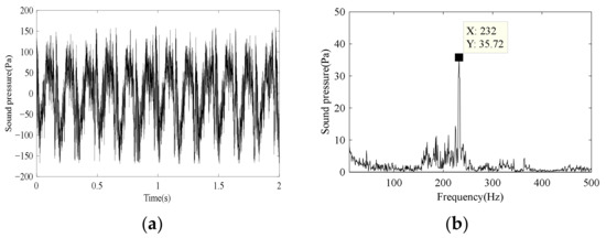
Figure 6.
Primary signal of the time-domain and the corresponding frequency spectrum of sound pressure: (a) Primary signal of the time-domain; (b) The corresponding frequency spectrum.
From Figure 6b, a crest value appears at 232 Hz that is around the tire acoustic cavity resonance frequencies of 237 Hz and 239.5 Hz [18], so the sound pressure and its spectrum of the tire cavity at the first-order acoustic resonance are captured.
3.1. Maximum Acoustic Pressure Amplitude in the TACRN
The noise emission is due to rolling and the air that expands behind the tire and is radiated noise outside the tire, and the research of this paper is the acoustic cavity resonance noise enclosed by the tire and wheel rim. The TACRN is transmitted into the car through the suspension and comes from the tire surface curvature change arising from the contact between the tire and road, road roughness and tread pattern. When the tire cavity resonance takes place, automobile tire resonates with the acoustic cavity, the acoustic pressure amplitude at each point of the acoustic cavity is different. For the first-order cavity resonance, the amplitudes of the sound pressure at two positions are largest. Theoretically, the amplitudes of the sound pressure spectrum at these two positions are same. Of course, the amplitudes of sound pressure at these two positions are slightly different due to element division. The position of the maximum sound pressure changes with the rotational speeds of the tire, but the maximum acoustic pressure amplitude changes slightly and is actually the maximum sound pressure which is extracted by software at a certain moment. The maximum sound pressure and distributions contour of the acoustic pressure amplitude are displayed in Figure 7 according to the operational conditions as displayed in Figure 5b. Besides, the maximum sound pressure in the TACRN is about 156 Pa.
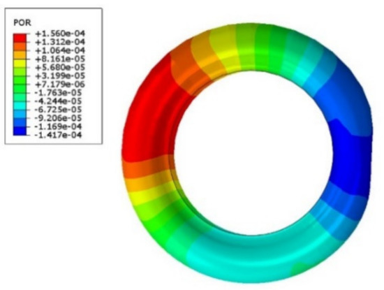
Figure 7.
Distributions contour of the acoustic pressure amplitude.
By using the same simulation means, the maximum acoustic pressure amplitudes under the factors of various loads, inflation pressures and running speeds are also calculated, and are shown in Table 3.
Table 3.
Maximum acoustic pressure amplitudes (Pa).
Base on Table 3, the effects of corresponding factors on the TACRN can be analyzed as follows.
3.2. Effects of Load and Experimental Validation
For the various running speeds, based on Table 3, the variations of maximum acoustic pressure amplitudes with loads are demonstrated in Figure 8.
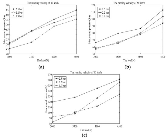
Figure 8.
Variation of maximum acoustic pressure amplitudes with the various loads: (a) For the running speed of 40 km/h; (b) For the running speed of 50 km/h; (c) For the running speed of 60 km/h.
Maximum acoustic pressure amplitude raises with the load from Figure 8. The main reason is that the increment of load leads to add of the area importing the energy, besides, the energy imported raises.
Figure 7 demonstrates the acoustic pressure distributions contour (modal shape) according to the previous operational conditions and Figure 9 is the acoustic pressure amplitude distributions in the polar coordinate. From Figure 9, the acoustic pressure amplitude decreases with the angle of rotation at first, then increases to maximum, and decreases again.
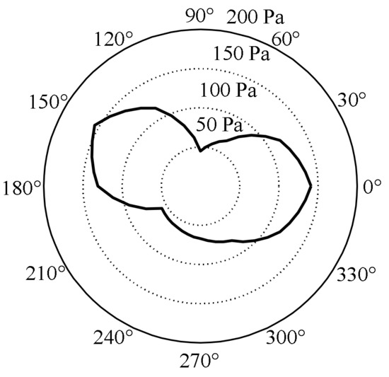
Figure 9.
The distributions of the acoustic pressure amplitude in the polar coordinate system for the load of 4500 N.
Figure 10a,b show the acoustic pressure distributions with various loads in Cartesian coordinate. There are twelve points with interval of 30 degrees in the polar coordinate, and the angular coordinates stand for various locations (0° means the centre of tire contact patch and 180° means the opposite location). The radius coordinates stand for the acoustic pressure amplitudes. Moreover, the abscissa stands for various locations (0° and 360° mean the center of tire contact patch) in the Cartesian coordinate, and the vertical coordinate stands for transient sound pressure in Figure 10a by reading the transient sound pressure value of corresponding position in the distribution contour while the vertical coordinate represents the acoustic pressure amplitudes in Figure 10b. The influence of the phase is introduced and causes the values in Figure 10a to appear positive or negative. If taking the value of Figure 10a in absolute terms, we get Figure 10b.
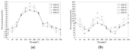
Figure 10.
The acoustic pressure distributions: (a) The transient sound pressure distributions; (b) The acoustic pressure amplitudes distributions.
Figure 10a indicates that there are one peak and one trough in the acoustic cavity and Figure 10b demonstrates that there are two troughs and two crest values. Based on the literature [18,19], the crest values are supposed to arise the positions of 0 degrees and 180 degrees, and the trough values should emerge the locations of 90 degrees and 270 degrees if the automobile tire does not rotate. In fact, since the anticlockwise rotation of the drum causes the velocity of the forward traveling wave (rotating in the same direction of the drum) in the cavity to be larger than the velocity of the backward traveling wave (rotating in the opposite direction), the peak appears near the position of 0 degree and 150 degree in Figure 10b.
From Figure 10b, acoustic pressure amplitude distribution for various loads have the analogical trend that the acoustic pressure amplitude reduces firstly, then raises to maximum, and reduces again.
In the previous literature [18], the authors have carried out an experimental study on TACRN under the same operating conditions as before are indicated in Figure 11. The sound pressure distribution was shown in Figure 11a,b, and the sound pressure distribution of Figure 9 is also shown in Figure 11a. Moreover, the RMS values between Figure 10b and Figure 11b are shown in Table 4.
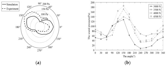
Figure 11.
The acoustic pressure amplitude distributions: (a) For the load of 4500 N; (b) For all these loads.
The tendency of the above simulation consequences as shown in Figure 11a,b is consistently same as that in Figure 9 and Figure 10b, respectively. Besides, the relative errors of RMS values between Figure 10b and Figure 11b are acceptable. Therefore, the simulation method has been validated by experiment.
3.3. Effects of Automobile Tire Inflation Pressure and Experimental Validation
For various loads undertaken by tire, based on Table 3, the maximum acoustic pressure amplitudes change with the automobile tire inflation pressures, which are displayed in Figure 12.
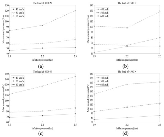
Figure 12.
Variation of maximum acoustic pressure amplitudes with inflation pressures: (a) For the load of 3000 N; (b) For the load of 3500 N; (c) For the load of 4000 N; (d) For the load of 4500 N.
From Figure 12, the maximum acoustic pressure amplitude at 2.5 bar is the largest compared with that at 2.2 bar and 1.9 bar for the identical load and running speed. The cause is that the increase in the automobile tire inflation pressure leads to an increase in tire stiffness.
Figure 13a shows distributions contour of acoustic pressure amplitude when the load is 3500 N and the running speed is 50 km/h for the automobile tire inflation pressure of 2.5 bar and Figure 13b is the corresponding distributions of the acoustic pressure amplitude in the polar coordinate. From Figure 13b, the acoustic pressure amplitude decreases with the angle of rotation at first, then increases to maximum, and decreases again.
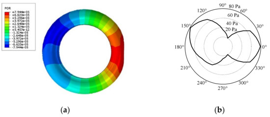
Figure 13.
The acoustic pressure distribution for the inflation pressure of 2.5 bar: (a) Distributions contour of the acoustic pressure amplitude; (b) Distributions of the acoustic pressure amplitude in the polar coordinate.
Figure 14a,b display the acoustic pressure amplitudes distributions when the load is 3500 N and the running speed is 50 km/h with various automobile tire inflation pressures in the Cartesian coordinate. The influence of the phase is introduced, which causes the values in Figure 14a to appear to be either positive or negative. If the values of Figure 14a are taken in absolute values, Figure 14b is developed.
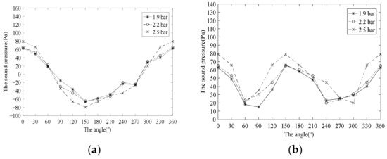
Figure 14.
The sound pressure distributions: (a) The transient acoustic pressure distributions; (b) The acoustic pressure amplitudes distributions.
From Figure 14a, there is one crest value and one trough, and Figure 14b indicates that there are two crest values and two troughs. In fact, the crest values arise near the positions of 0 degree and 150 degree, for the reason given in the previous section.
From Figure 14b, the acoustic pressure amplitude distributions for various automobile tire inflation pressures have the analogical trend.
In the previous literature [18], the authors carried out an experimental study on TACRN where the acoustic pressure amplitudes distributions under the identical operating conditions of Figure 13 are displayed in Figure 15a,b, and the sound pressure distribution of Figure 13b is also shown in Figure 15a. Moreover, the RMS values between Figure 14b and Figure 15b are shown in Table 5.
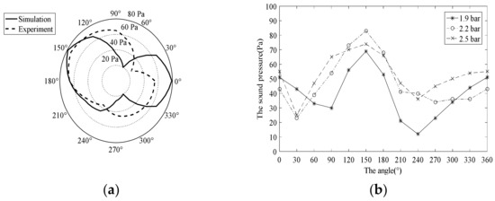
Figure 15.
The acoustic pressure amplitude distributions: (a) For the inflation pressure of 2.5 bar; (b) For all these inflation pressures.
The trend of the simulation consequences from Figure 15a,b, is consistent with that from Figure 13b and Figure 14b, respectively. Besides, the relative errors of RMS values between Figure 14b and Figure 15b are acceptable. Therefore, the simulation method has once again been validated by experiment.
In short, the maximum acoustic pressure amplitude of simulation is generally lower than the maximum acoustic pressure amplitude in the experiment for two reasons: firstly, the tire in the experiment has patterns, which can cause the additional excitation input, resulting in larger input energy. On the contrary, the tire in the simulation is set as smooth for convenience, so the effect of pattern is not introduced. Secondly, there exists the friction between the tire and the drum in the experiment, but not in the simulation.
4. Analysis of Effects of Running Speed on TACRN Based on Simulation
Through the previous simulation and experimental verification, it is shown that the proposed method is feasible. Therefore, the method can be applied to predict the characteristics of TACRN, especially it is applicable for the high-speed rotating tire which is difficult to be tested in the test rig.
For various tire inflation pressures, based on Table 3, the variations of maximum acoustic pressure amplitudes with the running speeds are indicated in Figure 16.
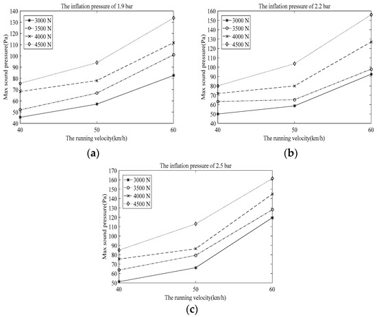
Figure 16.
Variation of maximum acoustic pressure amplitudes with running speeds: (a) For the inflation pressure of 1.9 bar; (b) For the inflation pressure of 2.2 bar; (c) For the inflation pressure of 2.5 bar.
The maximum acoustic pressure amplitude at the speed of 60 km/h is larger than those at the speed of 40 km/h and 50 km/h from Figure 16. The reason is that the rolling automobile tire could move the mass center of the cross section of acoustic cavity outward with the raised centrifugal force, furthermore, the energy simultaneously raises with the running speed.
Figure 17a presents distributions contour of acoustic pressure amplitudes when the tire inflation pressure is 2.2 bar and the load is 3000 N for the running velocity of 60 km/h, and Figure 17b indicates the corresponding distributions of the acoustic pressure amplitude in the polar coordinate. From Figure 17b, the acoustic pressure amplitude decreases with the angle of rotation at first, then increases to maximum, and decreases again.
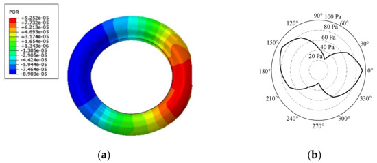
Figure 17.
Distribution of the acoustic pressure amplitude for the running speed of 60 km/h: (a) Distributions contour of the acoustic pressure amplitude; (b) Distributions of the acoustic pressure amplitude in the polar coordinate system.
Figure 18a,b presents acoustic pressure amplitude distribution when the automobile tire inflation pressure is 2.2 bar and the load is 3000 N with various running speeds in the Cartesian coordinate. The influence of the phase is introduced, which causes the values in Figure 18a to appear to be either positive or negative. If the value of Figure 18a is taken in the absolute value, Figure 18b is then obtained.
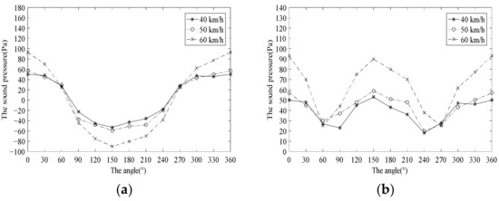
Figure 18.
The acoustic pressure amplitude distributions: (a) The transient sound pressure distributions; (b) The acoustic pressure amplitudes distributions.
It can be seen from Figure 18a that there are one crest value and one trough, and Figure 18b displays that there are two crest values and two troughs. In fact, the crest values arise near the positions of 0 degree and 150 degree, for the reasons given in the previous section.
From Figure 18b, the acoustic pressure amplitude distributions for various tire inflation pressures have the analogical trend.
According to operational conditions of Figure 17a, Figure 19 shows the acoustic pressure amplitude distribution where the drum excitation is located on tire at different positions. (The black arrow represents the excitation of the drum) From Figure 19, it is seen that although the loading position changes, but the distribution of sound pressure field with respect to the loading position is not changed. Therefore, the stability of the sound pressure field in the tire produces a stable vibration transmitted to the suspension system.
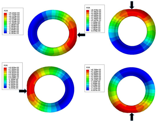
Figure 19.
Distribution contours of the sound pressure at different positions.
In order to further study the relationship between the location of the peaks and rotation direction of the tire, the roller drum is driven to rotate clockwise around the center axis of the spindle axle of the tire-wheel assembly. Figure 20a shows the distribution contour according to the operational conditions of Figure 17a, while Figure 20b indicates the corresponding distributions of the acoustic pressure amplitude in the polar coordinate.
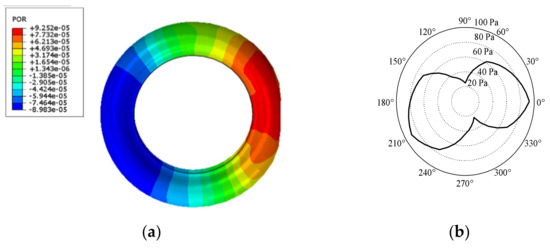
Figure 20.
The acoustic pressure amplitude distribution for the running speed of 60 km/h: (a) Distributions contour of the acoustic pressure amplitude; (b) The acoustic pressure amplitude distributions in the polar coordinate.
From Figure 20a, there is one peak and one trough, and Figure 20b demonstrates that there are two crest values and two troughs. In fact, since the clockwise rotation of the drum causes the velocity of the forward traveling wave (rotating in the same direction of the drum) in the cavity to be much larger than the velocity of the backward traveling wave (rotating in the opposite direction), the crest value appears near the locations of 0 degree and 210 degree in Figure 20b.
Due to the complicated experimental conditions, the experiment equipment cannot meet the requirements under certain operational conditions. For example, the sensor is difficult to accurately measure the sound pressure at a high rotating speed since the effect of a great centrifugal force. However, the simulation can effectively make up for this shortcoming. So based on the simulation, the sound pressure under the test condition difficult to be implemented can be analyzed.
Figure 21 shows the acoustic pressure amplitude distributions when the load is 3000 N and the running speeds is 80 km/h and 100 km/h for the automobile tire inflation pressure of 2.2 bar. From Figure 21, the maximum acoustic pressure amplitude is about 137.6 Pa and 171.6 Pa, respectively. It is also seen that the acoustic pressure amplitude distribution for higher running speeds have the analogical trend.
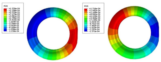
Figure 21.
The acoustic pressure amplitude distribution for the running speeds of 80 km/h and 100 km/h.
5. Conclusions
In this paper, a simulation method introducing the equivalent rotating condition is proposed to evaluate the sound field in rotating automobile tire cavity. The simulation consequences under different operational conditions are verified by experiments, and the comparison between the test and simulation consequences demonstrate that the simulation means provide a valid and correct tool for forecasting the sound field in the rotating tire. Furthermore, the influences of the running speed, the inflation pressure and the load on the sound field are analyzed according to the simulation consequences. In particular, the simulation of the operational condition difficult to be implemented and the mechanism of peak asymmetry effect based on the simulation are further studied. The related conclusions are as follows:
- (1)
- The running speed of vehicle has an important influence on the acoustic field. Besides, the counterclockwise revolution of drum which arouses the velocity of the forward traveling wave in the cavity to be higher than the velocity of the backward traveling wave give rise to that the crest values of acoustic pressure amplitude arise around the positions of 0 degrees and 150 degrees.
- (2)
- The inflation pressure, load and running speed of vehicle have various influence on the maximum acoustic pressure amplitude. The maximum acoustic pressure amplitude raises with the increase of the load and the running speed from the analysis of simulation and test. Besides, the maximum acoustic pressure amplitude raises with the increment of automobile tire inflation pressure from the analysis of simulation. However, the maximum acoustic pressure amplitude raises firstly and reduces again with the increment of automobile tire inflation pressure from the analysis of test.
- (3)
- The maximum acoustic pressure amplitude of simulation is generally lower than the maximum acoustic pressure amplitude of test.
Author Contributions
X.H. designed, carried out the test and simulation method, analyzed the data and wrote the paper, X.L., Y.S. and T.H. reviewed and revised the paper. All authors have read and agreed to the published version of the manuscript.
Funding
This study was supported by the National Natural Science Foundation of China, grant number 51675021.
Institutional Review Board Statement
Not applicable.
Informed Consent Statement
Not applicable.
Acknowledgments
We thank all the participants in this study.
Conflicts of Interest
The authors have no conflict of interest concerning this manuscript.
References
- Li, T.; Burdisso, R.; Sandu, C. Literature review of models on tire-pavement interaction noise. J. Sound. Vib. 2018, 420, 357–445. [Google Scholar] [CrossRef]
- Kropp, W. The influence of tyre cavity resonances on the exterior noise. In Proceedings of the 23rd International Congress on Acoustics, Aachen, Germany, 9–13 September 2019. [Google Scholar]
- O’Boy, D.J.; Walsh, S.J. Automotive tyre cavity noise modelling and reduction. In Proceedings of the 45th International Congress and Exposition on Noise Control Engineering INTER-NOISE, Hamburg, Germany, 21–24 August 2016. [Google Scholar]
- Kamiyama, Y. Development of twin-chamber on-wheel resonator for tire cavity noise. Int. J. Automot. Technol. 2018, 19, 37–43. [Google Scholar] [CrossRef]
- Scavuzzo, R.W.; Charek, L.T.; Sandy, P.M.; Shteinhauz, G.D. Influence of wheel resonance on tire acoustic cavity noise. SAE Trans. 1994, 103, 643–648. [Google Scholar]
- Gregoriis, D.D.; Naets, F.; Kindt, P.; Desmet, W. Development and validation of a fully predictive high-fidelity simulation approach for predicting coarse road dynamic tire/road rolling contact forces. J. Sound. Vib. 2019, 452, 147–168. [Google Scholar] [CrossRef]
- Mohamed, Z.; Wang, X.; Jazar, R. A survey of wheel tyre cavity resonance noise. Int. J. Veh. Noise Vib. 2013, 9, 276–293. [Google Scholar] [CrossRef]
- Mohamed, Z.; Wang, X.; Jazar, R. Structural-acoustic coupling study of tyre-cavity resonance. J. Vib. Control 2014, 22, 513–529. [Google Scholar] [CrossRef]
- Sakata, T.; Morimura, H.; Ide, H. Effects of tire cavity resonance on vehicle road noise. Tire Sci. Technol. 1990, 18, 68–79. [Google Scholar] [CrossRef]
- Thompson, J.K. Plane wave resonance in the tire air cavity as a vehicle interior noise source. Tire Sci. Technol. 1995, 23, 2–10. [Google Scholar] [CrossRef]
- Mohamed, Z.; Egab, L.; Wang, X. Tyre cavity coupling resonance and countermeasures. Appl. Mech. Mater. 2014, 471, 3–8. [Google Scholar] [CrossRef]
- Wang, X.; Mohamed, Z.; Ren, H.; Liang, X.Y.; Shu, H.L. A study of tyre, cavity and rim coupling resonance induced noise. Int. J. Veh. Noise Vib. 2014, 10, 25–50. [Google Scholar] [CrossRef]
- Peng, B.; Pang, J.; Gong, S.C.; Zhang, J. Modeling and experimental investigation of mechanism of tire cavity noise. In Proceedings of the 46th International Congress and Exposition on Noise Control Engineering INTER-NOISE, Hong Kong, China, 27–30 August 2017. [Google Scholar]
- Yi, J.J.; Liu, X.D.; Shan, Y.C.; Dong, H. Characteristics of sound pressure in the tire cavity arising from tire acoustic cavity resonance excited by road roughness. Appl. Acoust. 2019, 146, 218–226. [Google Scholar] [CrossRef]
- Tanaka, Y.; Horikawa, S.; Murata, S. An evaluation method for measuring SPL and mode shape of tire cavity resonance by using multi-microphone system. Appl. Acoust. 2016, 105, 171–178. [Google Scholar] [CrossRef]
- Feng, Z.C.; Gu, P.; Chen, Y.J.; Li, Z.B. Modeling and experimental investigation of tire cavity noise generation mechanisms for a rolling tire. Sae Int. J. Passeng. Cars Mech. Syst. 2009, 2, 1414–1423. [Google Scholar] [CrossRef]
- Feng, Z.C.; Gu, P. Modeling and experimental verification of vibration and noise caused by the cavity modes of a rolling tire under static loading. Sae Tech. Pap. 2011. [Google Scholar] [CrossRef]
- Hu, X.J.; Liu, X.D.; Wan, X.F.; Shan, Y.C.; Yi, J.J. Experimental analysis of sound field in the tire cavity arising from the acoustic cavity resonance. Appl. Acoust. 2020, 161, 107172. [Google Scholar] [CrossRef]
- Wan, X.F.; Liu, X.D.; Shan, Y.C.; Jiang, E.; Yuan, H.W. Numerical and experimental investigation on the effect of tire on the 13° impact test of automotive wheel. Adv. Eng. Softw. 2019, 133, 20–27. [Google Scholar] [CrossRef]
- Dong, H. Research on the mechanism and control methods of tire cavity resonance. Master’s Thesis, Department of Mechanical Engineering, Beihang University, Beijing, China, 2018. [Google Scholar]
- Dong, H.; Liu, Y.G.; Shan, Y.C.; Liu, X.D. Simulation and Experimental Investigation of the Resonance Reduction of A Tire Cavity Lined With Porous Materials. In Proceedings of the 46th International Congress and Exposition on Noise Control Engineering INTER-NOISE, Hong Kong, China, 27–30 August 2017. [Google Scholar]
Publisher’s Note: MDPI stays neutral with regard to jurisdictional claims in published maps and institutional affiliations. |
© 2021 by the authors. Licensee MDPI, Basel, Switzerland. This article is an open access article distributed under the terms and conditions of the Creative Commons Attribution (CC BY) license (http://creativecommons.org/licenses/by/4.0/).