Full Three-Dimensional Inverse Design Method for S-Ducts Using a New Dimensionless Flow Parameter


Abstract
:1. Introduction
2. Numerical Procedure
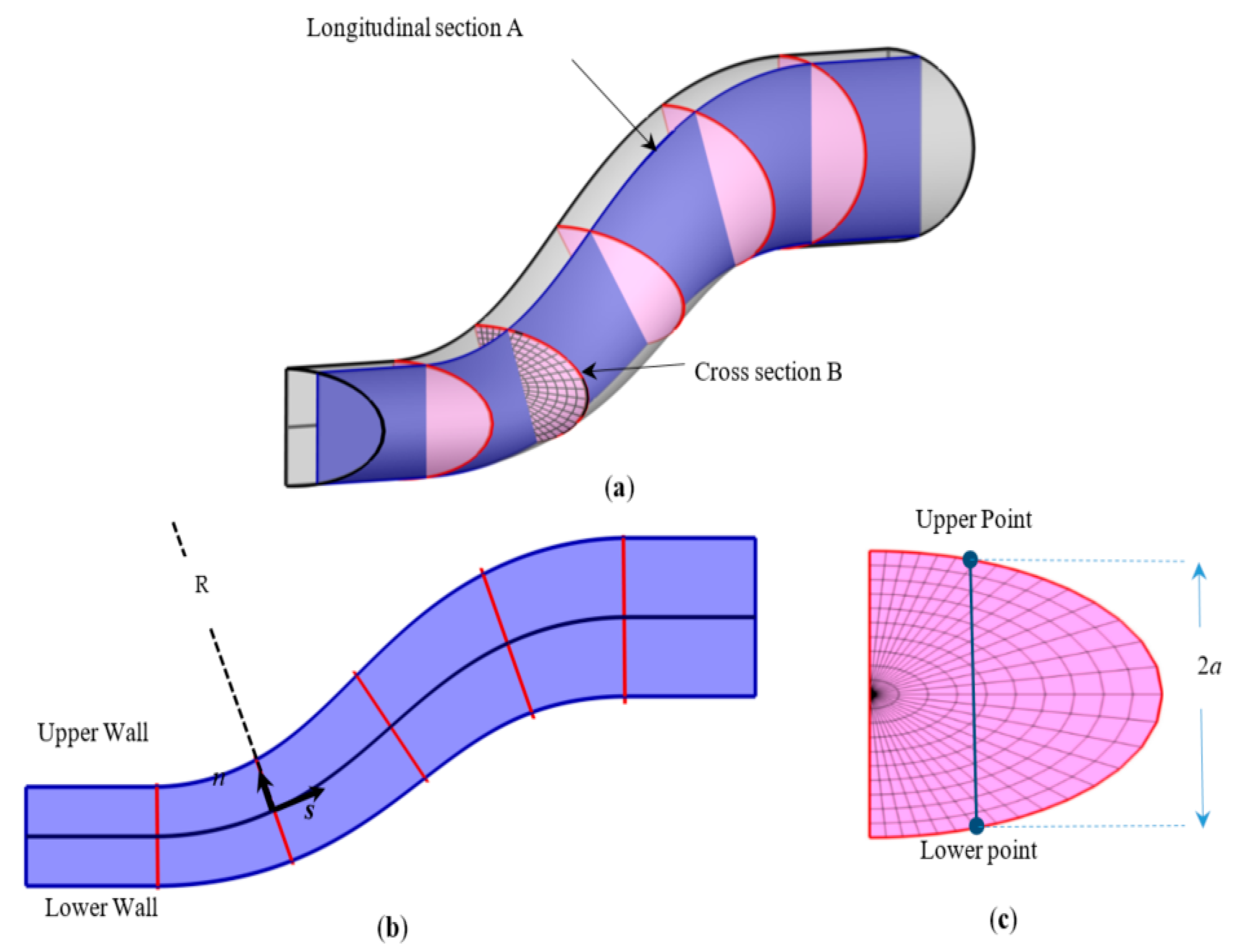
2.1. Flow Solver and Geometry Definition
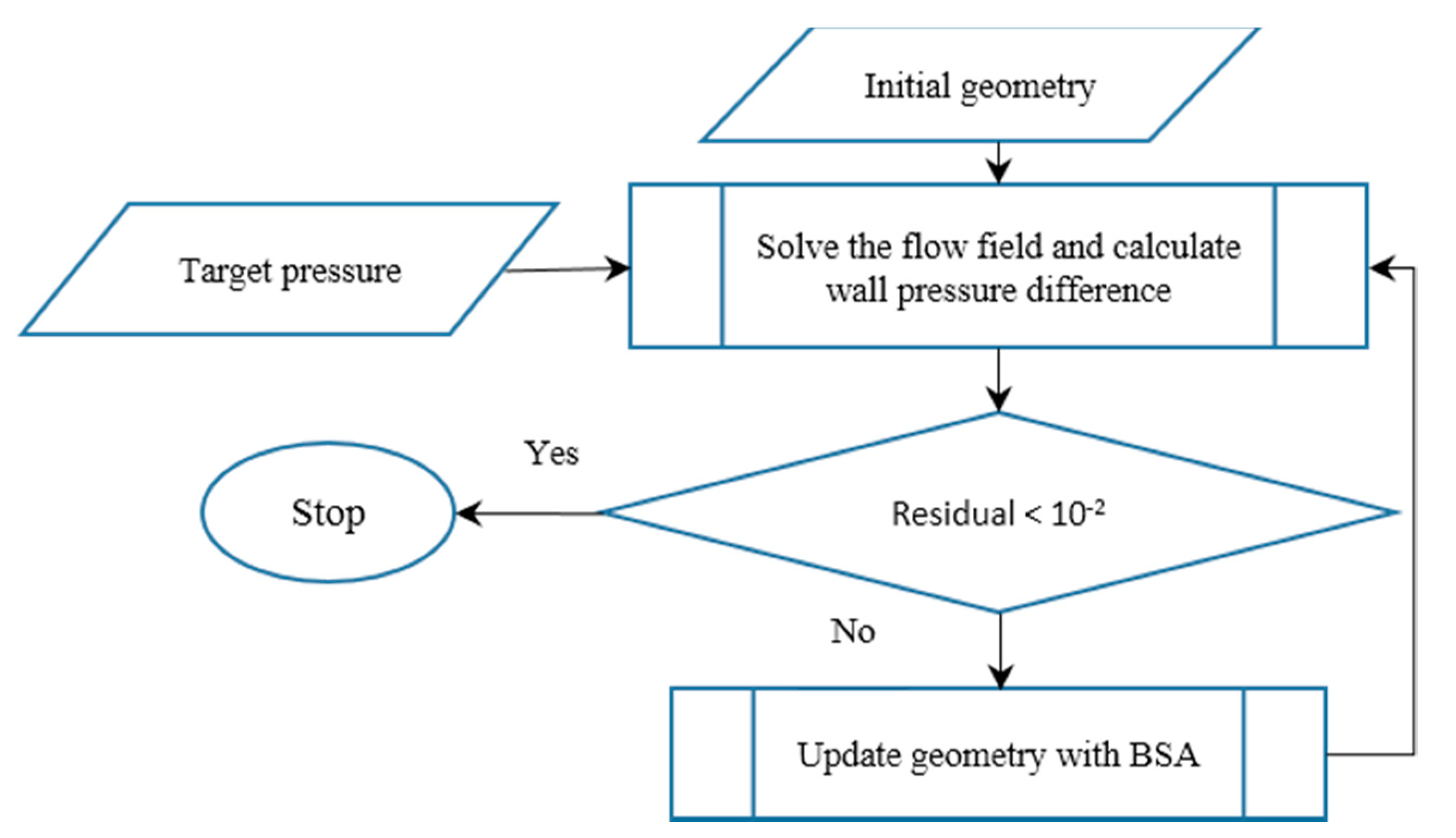
2.2. Inverse Design Method
2.3. Filtering Operation
3. Upgrading and Validating the 3-D BSA for Unique Solution
3.1. Definition of Curvature-Based Dimensionless Pressure Parameter for Upgrading the 3-D BSA
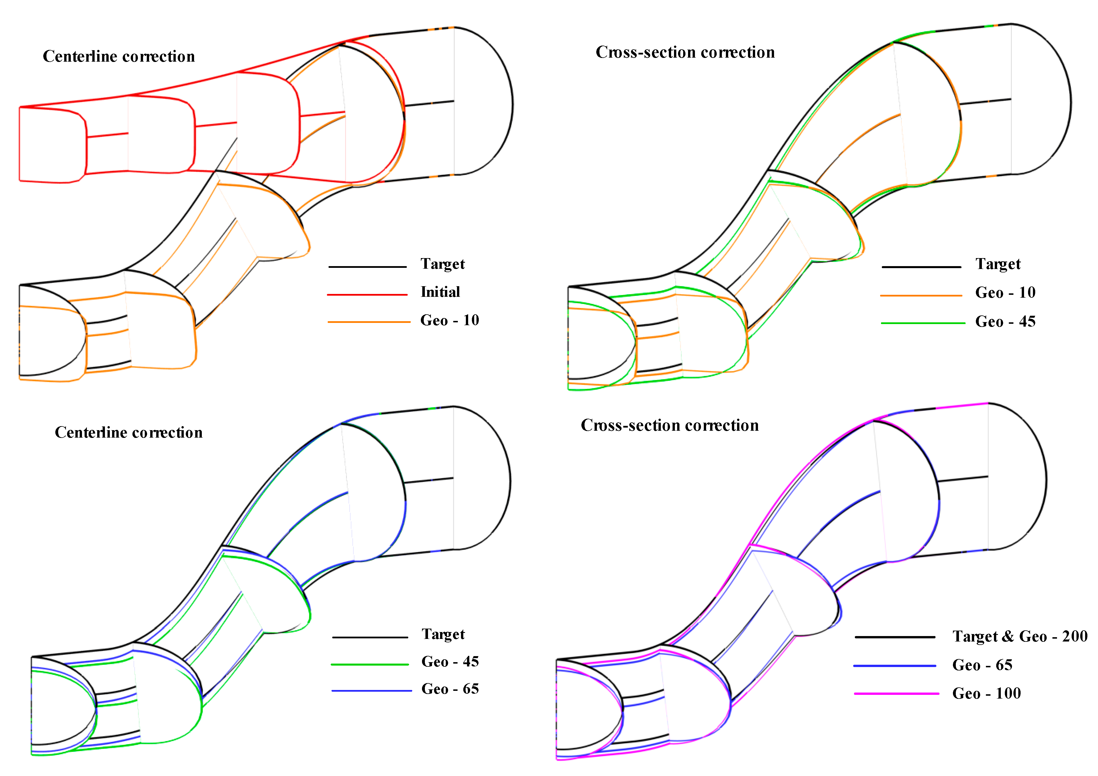
3.2. Correction of Cross Sections Based on Dimensionless Pressure
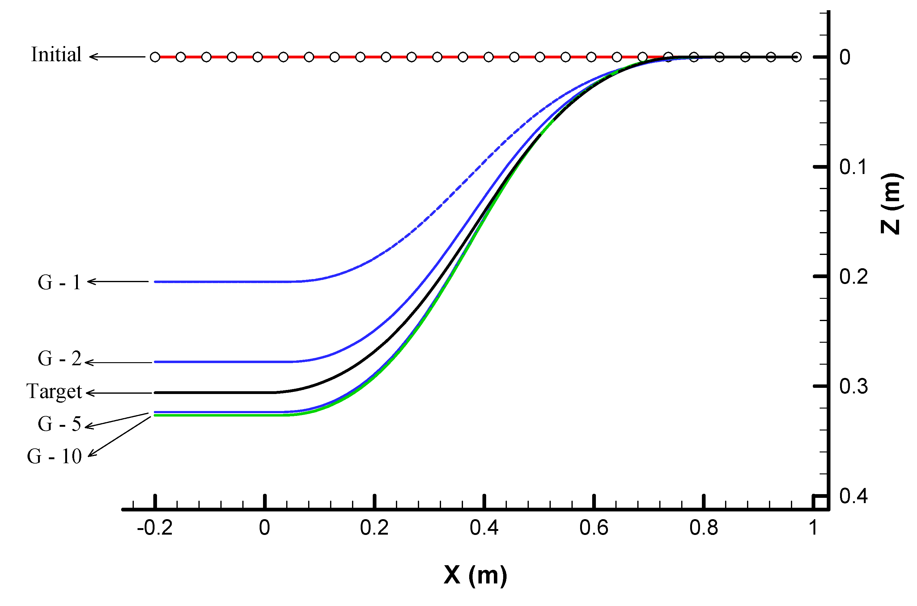
3.3. Correction of Centerline Curvature Based on Dimensionless Pressure
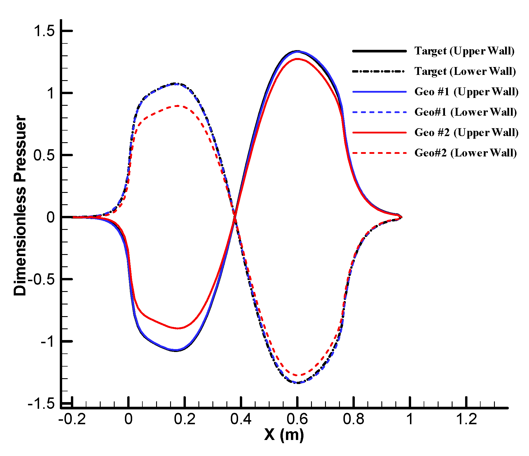
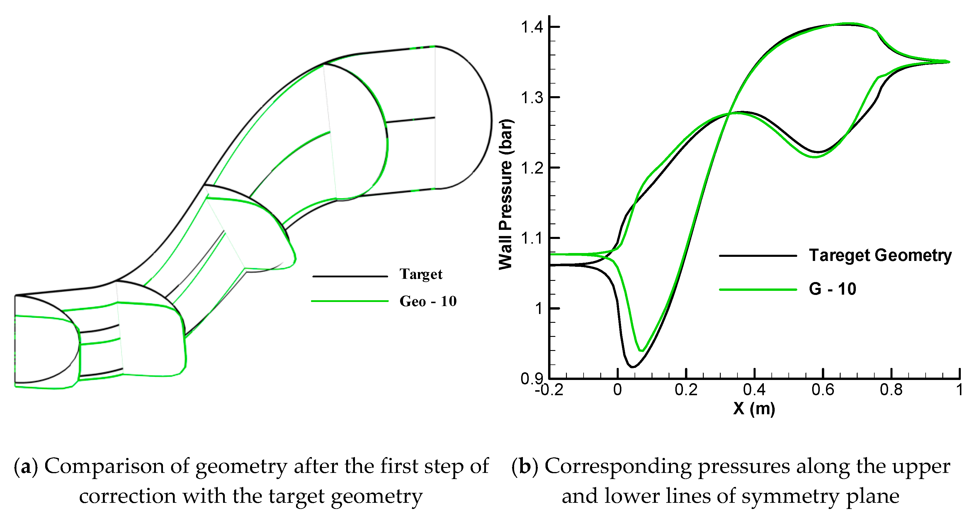
3.4. Validation of 3-D Upgraded Inverse Design for 3D S-Duct with Specified Centerline Curvature
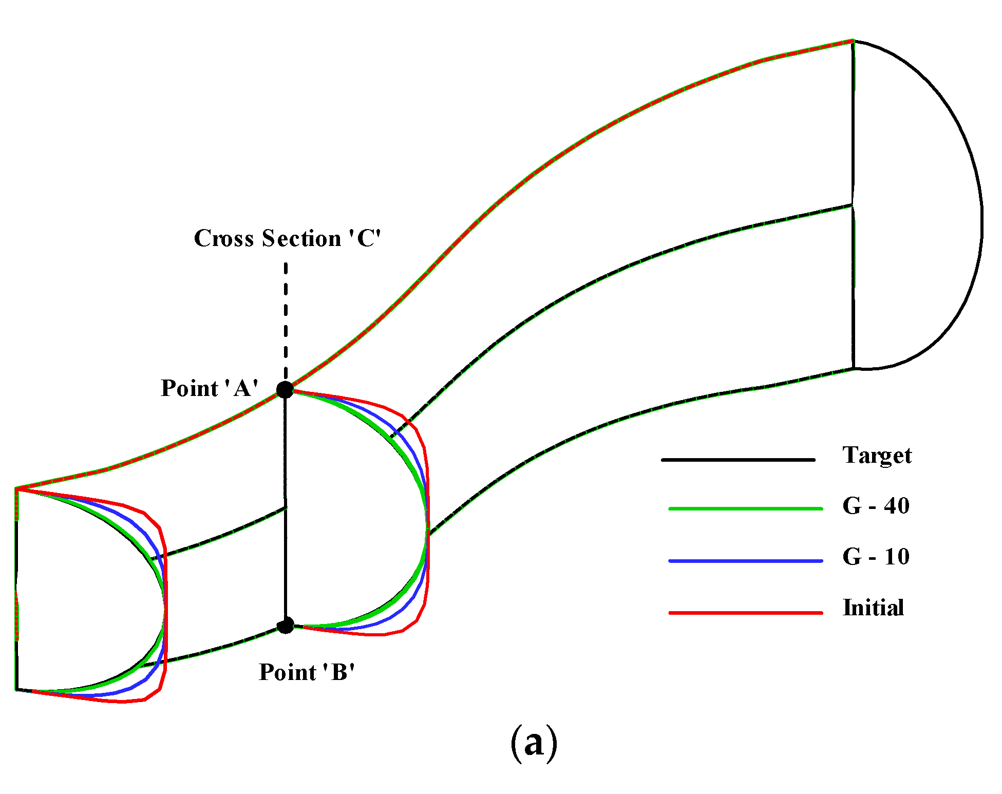
3.5. Validation of 3D Geometry with Desired Centerline Curvature
4. Design Example
5. Conclusions
Author Contributions
Funding
Conflicts of Interest
Nomenclature
| a | Half the cross-section height (m) |
| AR | Aspect ratio, height to length duct |
| b | Half the cross-section width (m) |
| BSA | Ball-spine algorithm |
| C | Geometry correction coefficient (m2s2/kg) |
| CPD | Current Pressure Distribution |
| DC (90) | Flow distortion |
| h | Duct height (m) |
| L | Duct length (m) |
| Number of nodes in axial direction | |
| Number of nodes in radial direction | |
| Number of nodes in azimuthal direction | |
| M | Mach number |
| P | Static pressure (Pa) |
| Total pressure (pa) | |
| Pressure of lower wall of 2D plannar duct | |
| Pressure of upper wall of 2D plannar duct | |
| R | Curvature of centerline |
| SSD | Surface shape design |
| TPD | Target Pressure Distribution |
| U | Flow velocity (m/s) |
| Velocity component in x-direction (m/s) | |
| Velocity component in y-direction (m/s) | |
| Velocity component in z-direction (m/s) | |
| Tangential velocity (m/s) | |
| W | Width of duct (m) |
| x | x coordinate |
| y | y coordinate |
| z | z coordinate |
| ΔP | Target and computed pressure difference (Pa) |
| Swirl angle (degree) | |
| θ | Angle between force vector and spine (rad) |
| Circumferential location (deg) | |
| Density (kg/m3) | |
| Subscripts | |
| 1 | Inlet condition |
| 2 | Outlet condition |
| ave | Average value |
| Comp | Computed conditions |
| Target | Target conditions |
References
- Ashrafizadeh, A.; Raithby, G.D.; Stubley, G.D. Direct design of airfoil shape with a prescribed surface pressure. Numer. Heat Transf. Part B Fundam. 2004, 46, 505–527. [Google Scholar] [CrossRef]
- Nili-Ahmadabadi, M.; Nematollahi, O.; Fatehi, M.; Cho, D.S.; Kim, K.C. Evaluation of aerodynamic performance enhancement of Risø_B1 airfoil with an optimized cavity by PIV measurement. J. Vis. 2020, 23, 591–603. [Google Scholar] [CrossRef]
- Stanitz, J.D. Design of Two-Dimensional Channels with Prescribed Velocity Distributions along the Duct Walls; Technical Report; US Government Printing Office: Washington, DC, USA, 1953; p. 1115.
- Stanitz, J.D. General Design Method for Three Dimensional, Potential Flow Fields, I—Theory; Technical Report; NASA: Washington, DC, USA, 1980; p. 3288.
- Zanetti, A. Natural formulation for the solution of two–dimensional or axis–symmetric inverse problems. Int. J. Numer. Methods Eng. 1986, 22, 451–463. [Google Scholar] [CrossRef]
- Ahmed, N.M.A.; Myring, D.F. An inverse method for the design of axisymmetric optimal diffuser. Int. J. Numer. Methods Eng. 1986, 22, 377–394. [Google Scholar] [CrossRef]
- Chaviaropoulos, P.; Dedoussis, V.; Papailiou, K.D. On the 3-D inverse potential target pressure problem. Part 1. Theoretical aspects and method formulation. J. Fluid Mech. 1995, 282, 131–146. [Google Scholar] [CrossRef]
- Chaviaropoulos, P.; Dedoussis, V.; Papailion, K.D. On the 3-D inverse potential target pressure problem. Part II: Numerical aspects and application to duct design. J. Fluid Mech. 1995, 282, 147–162. [Google Scholar] [CrossRef]
- Ashrafizadeh, A.; Raithby, G.D.; Stubley, G.D. Direct design of shape. Numer. Heat Transf. Part B Fundam. 2002, 41, 501–520. [Google Scholar] [CrossRef]
- Taiebi-Rahni, M.; Ghadak, F.; Ashrafizadeh, A. A direct design approach using the Euler equations. Inverse Probl. Sci. Eng. 2008, 16, 217–231. [Google Scholar] [CrossRef]
- Ghadak, F. A Direct Design Method Based on the Laplace and Euler Equations with Application to Internal Subsonic and Supersonic Flows. Ph.D. Thesis, Aero Space Department, Sharif University of Technology, Tehran, Iran, 2005. [Google Scholar]
- Ashrafizadeh, A.; Alinia, B.; Mayeli, P. A new co-located pressure-based discretization method for the numerical solution of incompressible Navier-Stokes equations. Numer. Heat Transf. Part B Fundam. 2015, 67, 563–589. [Google Scholar] [CrossRef]
- Rao, S.S. Engineering Optimization, Theory and Practice, 3rd ed.; Wiley: New York, NY, USA, 1996. [Google Scholar]
- ZiaeiRad, S.; Ziaei Rad, M. Inverse design of supersonic diffuser with flexible walls using a Genetic Algorithm. J. Fluids Struct. 2006, 22, 529–540. [Google Scholar] [CrossRef]
- Gan, W.; Zhang, X. Design optimization of a three-dimensional diffusing S-duct using a modified SST turbulent model. Aerosp. Sci. Technol. 2016, 63, 63–72. [Google Scholar] [CrossRef]
- Chiereghin, N.; Guglielmi, L.; Savill, M.; Kipouros, T.; Manca, E.; Rigobello, A.; Barison, M.; Benini, E. Shape Optimization of a Curved Duct with Free Form Deformations. In Proceedings of the 23rd AIAA Computational Fluid Dynamics Conference, Denver, CO, USA, 5–9 June 2017. [Google Scholar]
- Zeng, L.; Pan, D.; Ye, S. A fast multiobjective optimization approach to S-duct scoop inlets design with both inflow and outflow. Proceedings of the Institution of Mechanical Engineers, Part G. J. Aerosp. Eng. 2018, 233, 3381–3394. [Google Scholar]
- D’Ambros, A.; Kipouros, T.; Zachos, P.; Savill, M.; Benini, E. Computational design optimization for S-ducts. Designs 2018, 2, 36. [Google Scholar]
- Barger, R.L.; Brooks, C.W. A Streamline Curvature Method for Design of Supercritical and Subcritical Airfoils; TN D-7770; NASA: Washington, DC, USA, 1974.
- Garabedian, P.; Mcfadden, G. Design of supercritical swept wings. AIAA J. 1982, 20, 289–291. [Google Scholar] [CrossRef]
- Malone, J.; Vadyak, J.; Sankar, L.N. Inverse aerodynamic design method for aircraft components. J. Aircr. 1986, 24, 8–9. [Google Scholar] [CrossRef]
- Dulikravich, G.S.; Baker, D.P. Aerodynamic shape inverse design using a Fourier series method. AIAA J. 1999. AIAA 99-0185. Available online: https://maidroc.fiu.edu/wp-content/uploads/2012/05/033itp7.pdf (accessed on 26 January 2021). [CrossRef]
- Nili-Ahmadabadi, M.; Durali, M.; Hajilouy-Benisi, A.; Ghadak, F. Inverse design of 2-D subsonic ducts using flexible string algorithm. Inverse Probl. Sci. Eng. 2009, 17, 1037–1057. [Google Scholar] [CrossRef]
- Nili-Ahmadabadi, M.; Hajilouy, A.; Durali, M.; Ghadak, F. Duct design in subsonic and supersonic flow regimes with and without normal shock using flexible string algorithm. In Proceedings of the ASME Turbo Expo 2009, Orlando, FL, USA, 8–12 June 2009. GT2009-59744. [Google Scholar]
- Nili-Ahmadabadi, M.; Hajilouy-Benisi, A.; Ghadak, F.; Durali, M. A novel 2D incompressible viscous inverse design method for internal flows using flexible string algorithm. J. Fluids Eng. 2010, 132, 031401-1. [Google Scholar] [CrossRef]
- Nili-Ahmadabadi, M.; Durali, M.; Hajilouy-Benisi, A. A novel quasi 3-D design method for centrifugal compressor meridional plane. In Proceedings of the ASME Turbo Expo 2010: Power for Land, Sea, and Air, Glasgow, UK, 14–18 June 2010; GT2010-23341. pp. 919–931. [Google Scholar]
- Nili-Ahmadabadi, M.; Durali, M.; Hajilouy-Benisi, A. A novel aerodynamic design method for centrifugal compressor impeller. J. Appl. Fluid Mech. 2014, 7, 329–344. [Google Scholar]
- Nili-Ahmadabadi, M.; Poursadegh, F. Centrifugal compressor shape modification using a proposed inverse design method. J. Mech. Sci. Technol. 2013, 27, 713–720. [Google Scholar] [CrossRef]
- Nili Ahmadabadi, M.; Ghadak, F.; Mohammadi, M. Subsonic and transonic airfoil inverse design via Ball-Spine Algorithm. Comput. Fluids 2013, 84, 87–96. [Google Scholar] [CrossRef]
- Samadi Vaghefi, N.; Nili-Ahmadabadi, M.; Roshani, M.R. Optimal design of axe-symmetric diffuser via genetic algorithm and Ball-Spine inverse design method. In Proceedings of the The International Mechanical Engineering Congress & Exposition, Houston, TX, USA, 9–15 November 2012. IMECE2012-87924. [Google Scholar]
- Hoghooghi, H.; Nili-Ahmadabadi, M.; Manshadi, M.D. Optimization of a subsonic wind tunnel nozzle with low contraction ratio via ball-spine inverse design method. J. Mech. Sci. Technol. 2016, 30, 2059–2067. [Google Scholar] [CrossRef]
- Shumal, M.; Nili-Ahmadabadi, M.; Shirani, E. Development of the ball-spine inverse design algorithm to swirling viscous flow for performance improvement of an axisymmetric bend duct. Aerosp. Sci. Technol. 2016, 52, 181–188. [Google Scholar] [CrossRef]
- Mayeli, P.; Nili-Ahmadabadi, M.; Besharati-Foumani, H. Inverse shape design for heat conduction problems via the ball spine algorithm. Numer. Heat Transf. Part B Fundam. 2016, 69, 249–269. [Google Scholar] [CrossRef]
- Madadi, A.; Kermani, M.J.; Nili-Ahmadabadi, M. Aerodynamic design of S-shaped diffusers using ball–spine inverse design method. J. Eng. Gas Turbines Power 2014, 136, 122606. [Google Scholar] [CrossRef]
- Madadi, A.; Kermani, M.J.; Nili-Ahmadabadi, M. Applying the ball-spine algorithm to the design of blunt leading edge airfoils for axial flow compressors. J. Mech. Sci. Technol. 2014, 28, 4517–4526. [Google Scholar] [CrossRef]
- Madadi, A.; Kermani, M.J.; Nili-Ahmadabadi, M. Application of an inverse design method to meet a target pressure in axial-flow compressors. Turbo Expo Power Land Sea Air 2011, 54679, 1315–1322. [Google Scholar]
- Madadi, A.; Kermani, M.J.; Nili-Ahmadabadi, M. Application of the ball-spine algorithm to design axial-flow compressor blade. Sci. Iran. 2014, 21, 1981–1992. [Google Scholar]
- Madadi, A.; Kermani, M.J.; Nili-Ahmadabadi, M. Three-dimensional design of axial flow compressor blades using the ball-spine algorithm. J. Appl. Fluid Mech. 2015, 8, 683–691. [Google Scholar] [CrossRef]
- Hesami, H.; Mayeli, P. Development of the ball-spine algorithm for the shape optimization of ducts containing nanofluid. Numer. Heat Transf. Part A Appl. 2016, 70, 1371–1389. [Google Scholar] [CrossRef]
- Safari, M.; Nili-Ahmadabadi, M.; Ghaei, A.; Shirani, E. Inverse design in subsonic and transonic external flow regimes using Elastic Surface Algorithm. Comput. Fluids 2014, 102, 41–51. [Google Scholar] [CrossRef]
- Nasrazadani, S.H.; Nili-Ahmadabadi, M.; Noorsalehi, M.H. Upgrade and development of elastic surface inverse design method for axial compressor cascade with sharp-edged blades. Numer. Heat Transf. Part B Fundam. 2020, 77, 64–86. [Google Scholar] [CrossRef]
- Roe, P.L. Approximate Riemann Solvers, Parameter Vectors, and Difference Schemes. J. Comput. Phys. 1981, 43, 357–372. [Google Scholar] [CrossRef]
- Bromba, M.U.A.; Ziegler, H. Application Hints for Savitzky-Golay Digital Smoothing Filters. Anal. Chem. 1981, 53, 1583–1586. [Google Scholar] [CrossRef]
- Press, W.H.; Teukolsky, S.A. Savitzky-Golay Smoothing Filters. Comput. Phys. 1990, 4, 669–672. [Google Scholar] [CrossRef]
- Marchlewski, K.; Łaniewski-Wołłk, Ł.; Kubacki, S. Aerodynamic Shape Optimization of a Gas Turbine Engine Air-Delivery Duct. J. Aerosp. Eng. 2020, 33, 04020042. [Google Scholar] [CrossRef]
- Zhang, J.M.; Wang, C.F.; Lum, K.Y. Multidisciplinary design of S-shaped intake. In Proceedings of the 26th AIAA Applied Aerodynamics Conference, Honolulu, HI, USA, 18–21 August 2008. AIAA-2008-7060. [Google Scholar]
- Fiola, C.; Agarwal, R.K. Simulation of secondary and separated flow in a diffusing S-duct using four different turbulence models. Proc. Inst. Mech. Eng. Part G J. Aerosp. Eng. 2014, 228, 1954–1963. [Google Scholar] [CrossRef]


| n = −4 | n = −3 | n = −2 | n = −1 | n = 0 | n = 1 | n = 2 | n = 3 | n = 4 | |||
|---|---|---|---|---|---|---|---|---|---|---|---|
| For the beginning points | 0 | 4 | − | − | − | − | 31 | 9 | −3 | −5 | 3 |
| 1 | 3 | − | − | − | 9 | 13 | 12 | 6 | −5 | − | |
| For the middle points | 2 | 2 | − | − | −3 | 12 | 17 | 12 | −3 | − | − |
| For the end points | 3 | 1 | − | −5 | 6 | 12 | 13 | 9 | − | − | − |
| 4 | 0 | 3 | −5 | −3 | 9 | 31 | − | − | − | − |
| Parameter | Present Study | D’Ambros et al. [18] | ||
|---|---|---|---|---|
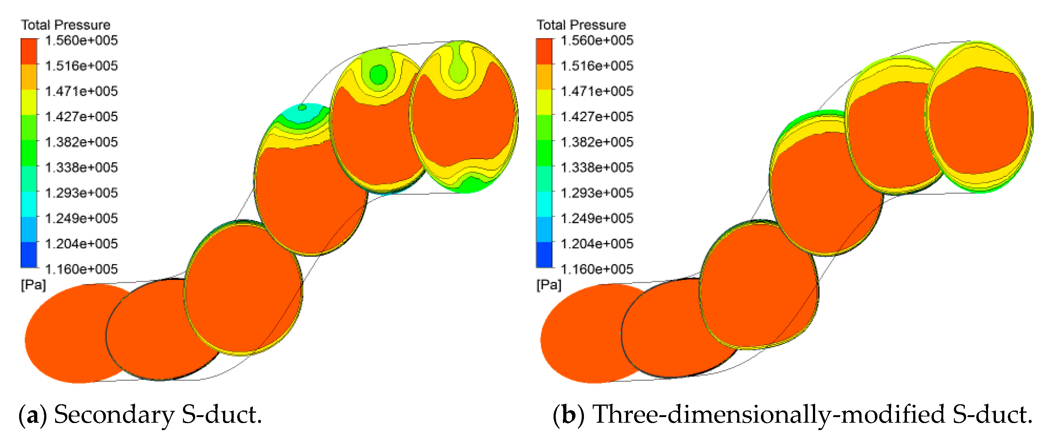
| Secondary | 3-D-Modified | |||
| Aspect ratio, AR = h/L | 0.41 | 0.41 | 0.27 | 0.27 |
| 0.264 | 0.085 | − | − | |
| Pressure recovery coefficient | 0.393 | 0.473 | 0.491 | 0.491 |
| Total pressure loss | 3.01 | 2.12 | 2.52 | 2.75 |
| Swirl angle | 1.096 | 0.861 | 3.256 | 1.411 |
Publisher’s Note: MDPI stays neutral with regard to jurisdictional claims in published maps and institutional affiliations. |
© 2021 by the authors. Licensee MDPI, Basel, Switzerland. This article is an open access article distributed under the terms and conditions of the Creative Commons Attribution (CC BY) license (http://creativecommons.org/licenses/by/4.0/).
Share and Cite
Kariminia, A.; Nili-Ahmadabadi, M.; Kim, K.C. Full Three-Dimensional Inverse Design Method for S-Ducts Using a New Dimensionless Flow Parameter. Appl. Sci. 2021, 11, 1119. https://doi.org/10.3390/app11031119
Kariminia A, Nili-Ahmadabadi M, Kim KC. Full Three-Dimensional Inverse Design Method for S-Ducts Using a New Dimensionless Flow Parameter. Applied Sciences. 2021; 11(3):1119. https://doi.org/10.3390/app11031119
Chicago/Turabian StyleKariminia, Atefeh, Mahdi Nili-Ahmadabadi, and Kyung Chun Kim. 2021. "Full Three-Dimensional Inverse Design Method for S-Ducts Using a New Dimensionless Flow Parameter" Applied Sciences 11, no. 3: 1119. https://doi.org/10.3390/app11031119
APA StyleKariminia, A., Nili-Ahmadabadi, M., & Kim, K. C. (2021). Full Three-Dimensional Inverse Design Method for S-Ducts Using a New Dimensionless Flow Parameter. Applied Sciences, 11(3), 1119. https://doi.org/10.3390/app11031119