Article

Inductive Thermography as Non-Destructive Testing for Railway Rails

1
Materials Center Leoben, 8700 Leoben, Austria
2
Chair of Automation, University of Leoben, 8700 Leoben, Austria
*
Author to whom correspondence should be addressed.
Appl. Sci. 2021, 11(3), 1003; https://doi.org/10.3390/app11031003
Submission received: 27 November 2020 / Revised: 12 January 2021 / Accepted: 14 January 2021 / Published: 22 January 2021
(This article belongs to the Special Issue Infrared Imaging and NDT)

Abstract

:
Inductive thermography is a non-destructive testing method, whereby the specimen is slightly heated with a short heating pulse (0.1–1 s) and the temperature change on the surface is recorded with an infrared (IR) camera. Eddy current is induced by means of high frequency (HF) magnetic field in the surface ‘skin’ of the specimen. Since surface cracks disturb the eddy current distribution and the heat diffusion, they become visible in the IR images. Head checks and squats are specific types of damage in railway rails related to rolling contact fatigue (RCF). Inductive thermography can be excellently used to detect head checks and squats on rails, and the method is also applicable for characterizing individual cracks as well as crack networks. Several rail pieces with head checks, with artificial electrical discharge-machining (EDM)-cuts and with a squat defect were inspected using inductive thermography. Aiming towards rail inspection of the track, 1 m long rail pieces were inspected in two different ways: first via a ‘stop-and-go’ technique, through which their subsequent images are merged together into a panorama image, and secondly via scanning during a continuous movement of the rail. The advantages and disadvantages of both methods are compared and analyzed. Special image processing tools were developed to automatically fully characterize the rail defects (average crack angle, distance between cracks and average crack length) in the recorded IR images. Additionally, finite element simulations were used to investigate the effect of the measurement setup and of the crack parameters, in order to optimize the experiments.

1. Introduction

Head checks and squats are common defects on rails stemming from rolling contact fatigue (RCF) [1,2,3,4]. Head checks are a material fatigue phenomenon caused by the high contact stresses between the wheel and the gauge corner of the rail. This mainly affects sections of track with a curve radius between 500 m and 3000 m, as the gauge corner on the outer rail is particularly stressed here. Due to the prevailing load conditions in normal railroad operation, there is a constant overstressing of the rail material, which reacts with a superficial hardening (work hardening) and is consequently accompanied by material fatigue. This is shown by the formation of externally visible, fine surface cracks occurring at discrete intervals, which are called head checks. Under continuous load, head checks grow into the rail head with a very shallow entry angle (10°–30°). After a certain amount of crack propagation, head checks tend to bend and continue to grow in the base material at a steeper angle, which can ultimately lead to fracture of the rail [3,5]. Consequently, railway infrastructure managers need measurement methods able to detect head checks in the early stage of their development and to assess their depth and inclination angles in order to schedule appropriate preventive maintenance measures such as rail grinding or, in extreme cases, rail milling [4].
Squats are rolling contact fatigue RCF defects occurring in straight or (gently) curved track within the running band on the rail head where the rail is heavily sheared. This specific defect phenomenon is thought to initiate via small bits of hard material (such as pieces of track ballast) that are caught between rail and wheel and cause one crack to grow rather than another. The crack then preferentially grows in the direction of the heavily sheared surface layer; this generates the characteristic round shape of the squat. A striking description of the rail damage pattern “squats” can be found in Reference [6]. For a detailed investigation Simon et al. [2] partitioned the rail head around a squat defect in several strips in longitudinal and transversal direction and investigated them by optical and by scanning electron microscopy. They summarized their observations in a schematic diagram that allows a better understanding of the layout of the rail surface with the directions of the microstructure deformation and the location of the squat initiation. The relevant literature on squats allows the conclusion that the residual stress state below the rail surface after operations is a main key to understanding the problem. However, currently only hypotheses are available to explain how squats are initiated or are able to grow from initial damages. Non-destructive testing methods able to detect squats and to elucidate the development of subsurface cracks around the squats are highly needed to understand this damage phenomenon and its evolution over load cycles, and to subsequently define adequate rail maintenance measures, e.g., the ones proposed by Stock et al. [4].
Nowadays railway rails are usually tested by ultrasound or by eddy current testing methods in order to detect rail defects [7]. Additionally, visual inspection, at least in laboratory conditions, can be very helpful to characterize the rail damage [1]. The traditional ultrasound testing requires a coupling medium such as water in order to induce the ultrasonic waves in the work-piece to be tested. Novel techniques were developed to generate ultrasonic waves without a coupling medium, as e.g., it has been demonstrated that electromagnetic acoustic transducers (EMAT) can be used to induce Rayleigh surface waves in the rail for detecting defects [8]. It is also possible to generate ultrasonic waves by laser pulses, which were presented for defect detection in railway axles and wheels [9,10].
In the last few years the new technique of inductive thermography has been developed, which has a high potential for automated rail inspection [11,12,13,14]. In the case of inductive thermography, the specimen to be tested is heated with a short inductive heating pulse, usually in the range of 0.1–1 s. The applied excitation frequency is in the range of 100–200 kHz, whereby in ferro-magnetic steel the induced eddy current penetrates only up to about 0.03 mm below the surface. Surface cracks, as e.g., head checks, disturb the eddy current distribution and also the heat diffusion, therefore they become visible in the infrared (IR) images, recorded by an IR camera. After evaluating this IR sequence, the cracks can be easily detected. In the last few years several publications have proved [15,16,17,18,19] that inductive thermography is able to localize surface cracks in metals. For industrial applications it is important that an inspection technique is standardized, and this was recently done by the German Institute for Standardization (DIN) [20].
In this paper we present the results of an inductive thermography inspection and we show that it is an excellent tool for characterization of the rail. Defects such as head checks and squats can be localized in a quick, contact-free and non-destructive way. Additionally, the defects can be characterized in a fully automated way by determining e.g., the number of head checks, their inclination angle and their length. The big advantage of this method, compared to traditional inspections as ultrasonic and eddy current testing, is that it delivers an image of the rail, showing the information from the surface along with additional information from a thin, 1–2 mm thick layer below the surface, which is relevant for these kinds of defects. The technique is quick (to inspect a 30 cm long rail piece needs less than 0.5 s) and the resulting phase image is easily understandable.
Several different rail pieces were tested in the laboratory, having a length in the range of 10 cm up to 1 m. To inspect them two different kinds of measurement techniques have been developed. The first technique is a stop-and-go technique where the images of static, consecutive measurements are merged to form a panorama image. In the case of the second ‘scanning’ technique the rail is inspected during a continuous movement. These two techniques are compared and their advantages and disadvantages explained.
Finite element simulations were carried out using the multi-physics package ANSYS. The goal of the simulations was, on the one hand, to achieve a better understanding of the physical processes, how the eddy current distribution and the heat diffusion are disturbed by the cracks. On the other hand, the simulations were used to investigate the influence of the cracks’ properties, i.e., crack depth and inclination angle, on the results. Additionally, the influence of the measurement parameters, i.e., the excitation frequency and heating pulse duration, were investigated in order to optimize the experimental setup and the crack detectability.

2. Inductive Thermography Measurements

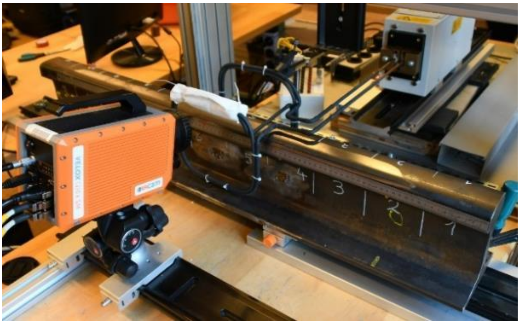
2.1. Description of the Laboratory Setup

The principle laboratory setup consists of an induction generator with an induction coil and an infrared camera (see Figure 1). Two setups for measuring railway rails were used: a static setup where equipment and specimen stayed in place and a scanning setup where the rail was moved at constant speed during measurement. A more detailed description of the two measurement setups is given in Section 6.3.
In the static setup a generator with a power output up to 10 kW was used. A short heating pulse of 0.1–0.2 s was applied to the rail sample through a Helmholtz coil, as is shown in Figure 1. The scanning setup was carried out by using a 5 kW generator with a linear coil. Both generators worked in the excitation frequency range of 100–200 kHz.
An infrared camera (IRCAM Velox 1310 k SM) recorded the surface temperature of the specimen during and after the heating pulse. This cooled IR camera with an InSb detector has 1280 × 1024 pixels, it is sensitive in the range of 1.5–5.1 µm and its noise equivalent temperature difference (NETD) is less than 25 mK. In full window mode it can record 180 images/s, but by using the binning mode and merging four pixels to one, the recording frequency increases up to 600 images/s. The IR camera and the induction generator were controlled and synchronized by a PLC. The recorded IR sequence was evaluated on a PC by software based on MATLAB, developed by the Chair of Automation of the University of Leoben.

2.2. Evaluation of Measurements to Phase Images

The IR camera records the surface temperature during the heating pulse as well as the cooling period after switching off the heating. For the desired crack detection a small temperature increase of 1–2 °C is enough, as can be seen in Figure 2b. Figure 2a shows that cracks on the surface are slightly more heated than the surrounding material. However, it is difficult to detect head checks in a single temperature image as e.g., in the top image of Figure 2a.
To improve the detectability of surface cracks a Fourier transformation of the recorded image sequence is performed for each pixel [15,21]:
F τ = 0 τ T t e i 2 π t / τ d t ,     Φ = arctan Im F τ Re F τ
where τ = tpulse + tcooldown and tcooldown is usually taken in the range of tpulse/2 and tpulse. In this study tcooldown = tpulse was chosen, but the selection of tcooldown = tpulse/2 leads to very similar results to the presented ones. In the bottom image of Figure 2a, the resulting phase image is shown. A phase image emphasizes the differences in the temperature increase during the heating as well as during the cool-down for each pixel. The effect of inhomogeneous heating and inhomogeneous surface property as emissivity is strongly decreased by the transformation [15,21] and the noise in the image is reduced, resulting in a higher signal-to-noise ratio [22].

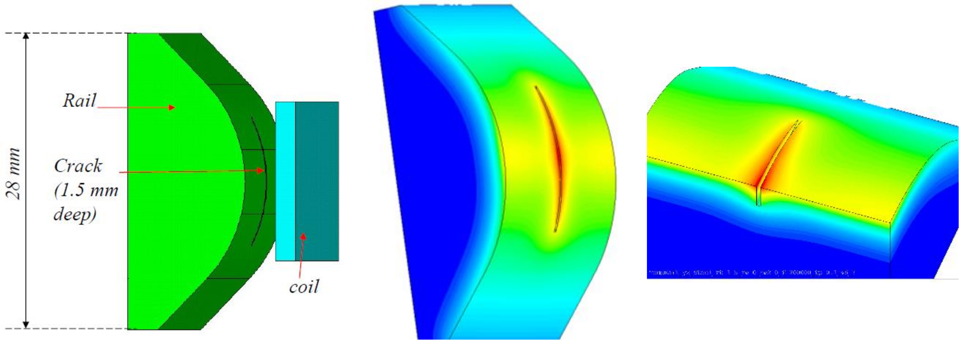
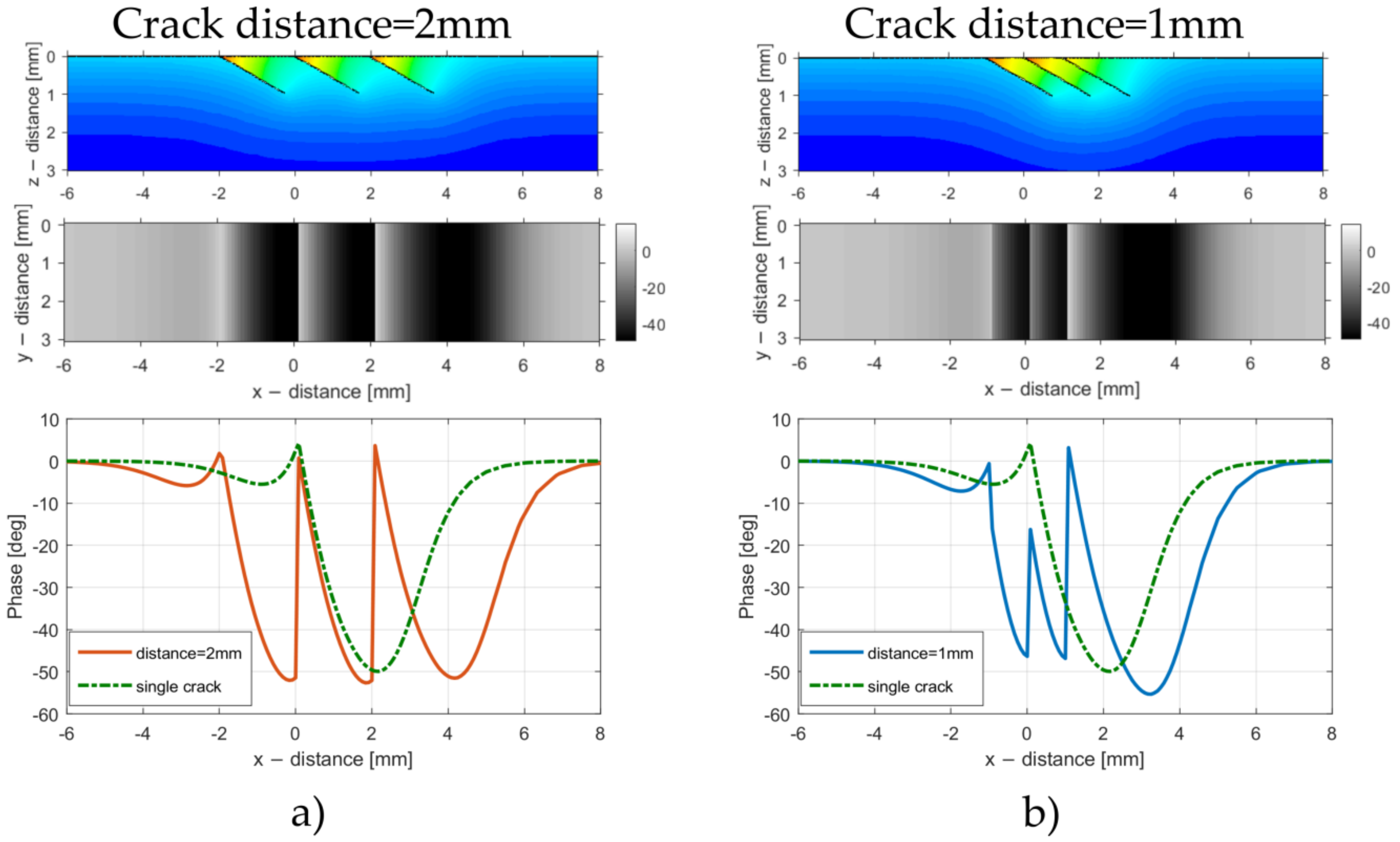
3. Finite Element Simulations

The ANSYS multiphysics simulation package [23] was used to model the inductive thermography measurements of the head checks in the rail. This package has the advantage that different physical phenomena can be simulated in a coupled way, as in this case electromagnetic induction is coupled with thermal calculation. In the first step inductive heating and the distribution of the induced eddy currents are modelled. Based on these results the Joule heating is calculated. In a further step the heat flow due to the generated Joule heating is modelled. The left image in Figure 3 shows the geometrical model of the gauge corner, where typically the head checks occur. The images in the middle and on the right side of Figure 3 show the temperature distribution after 0.1 s inductive heating pulse around a crack, which has at the deepest position 1.5 mm depth. The excitation frequency in the simulation model was 200 kHz and typical pearlitic steel material parameters were used for the rail piece. With these parameters the penetration depth of the eddy current is about 0.03 mm. As this depth is much less than the defect depth, the induced eddy currents flow around the defect, causing a higher current density and higher Joule heating in the vicinity of the crack. Additionally, the heat flow is also hampered by the crack and due to the heat accumulation the region around the crack has a higher temperature than the surrounding surface.
The simulation was set up using 3D hexahedral grids with 20-node elements. The size of the grid was about 0.01 mm in the region close to the surface and around the crack, and the grid size continuously increased towards the regions far away from the crack with a maximum element size of 0.6 mm. The electromagnetic part of the model consists of 296,000 elements, of which 134,000 are modeling the rail piece, 12,000 the induction coil and 150,000 the surrounding air. The thermal modelling was only performed for the work-piece part; the elements of the coil and the air were not included in the thermal calculation.
Several different numerical models were set up by varying the defect depth, its inclination angle below the surface and it’s angle at the surface regarding the gauge corner. Further simulation results are presented in Section 5. The temporal change of the simulated temperature was also evaluated by Fourier transformation and this phase image was then compared to the experimental results. The goal of the finite element simulations was to investigate the influence of the crack parameters on the phase distribution. For artificial cracks with known characteristics the simulated and the experimental results can be easily compared, which was used to validate the simulation models. In a further step, this supports the usage of the simulation results also for real cracks where the depth and inclination angle below the surface are not known so that they can be estimated from the simulations. Additional models were also set up, varying the heating pulse duration and the excitation frequency [15]. These models were used to optimize the experimental setup, resulting in the usage of 200 kHz as the excitation frequency and a heating pulse duration between 0.1 and 0.2 s.

4. Reference Rail Piece with Artificial Cracks

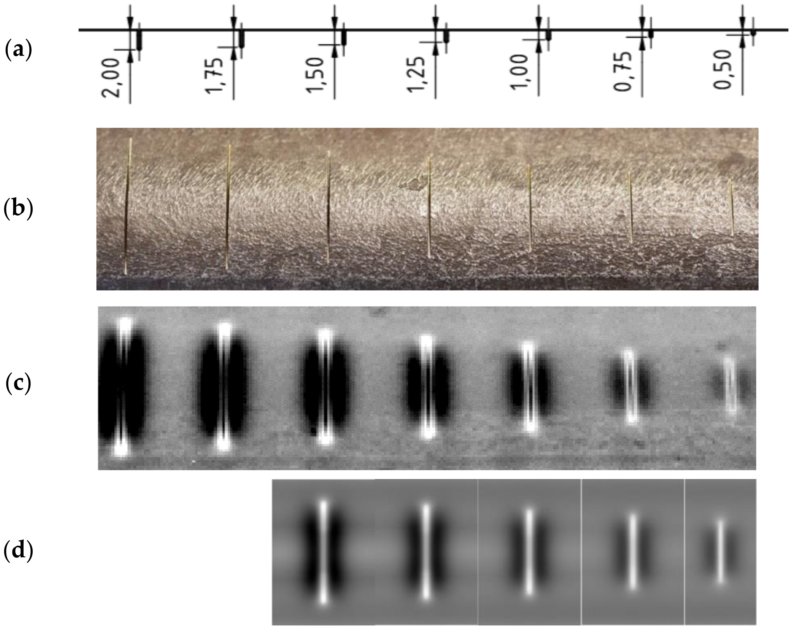
4.1. Vertical EDM-Cuts with Different Depths

To verify the simulation results, a reference rail piece (RP01) with artificial cracks was created. In an intact piece of a rail with a length of 10 cm, several cuts at the gauge corner were manufactured by the technique of electrical discharge-machining (EDM). On one side the cuts were perpendicular to the surface, as is shown in Figure 4a.
The resulting phase image of the thermographic measurement, as well as a photo of the vertical cuts at the gauge corner, can be seen in Figure 4. It noteworthy that as the cuts were created in the curved region of the rail, the deeper the cracks are, the longer they are at the surface. In the phase image the following features can be recognized:
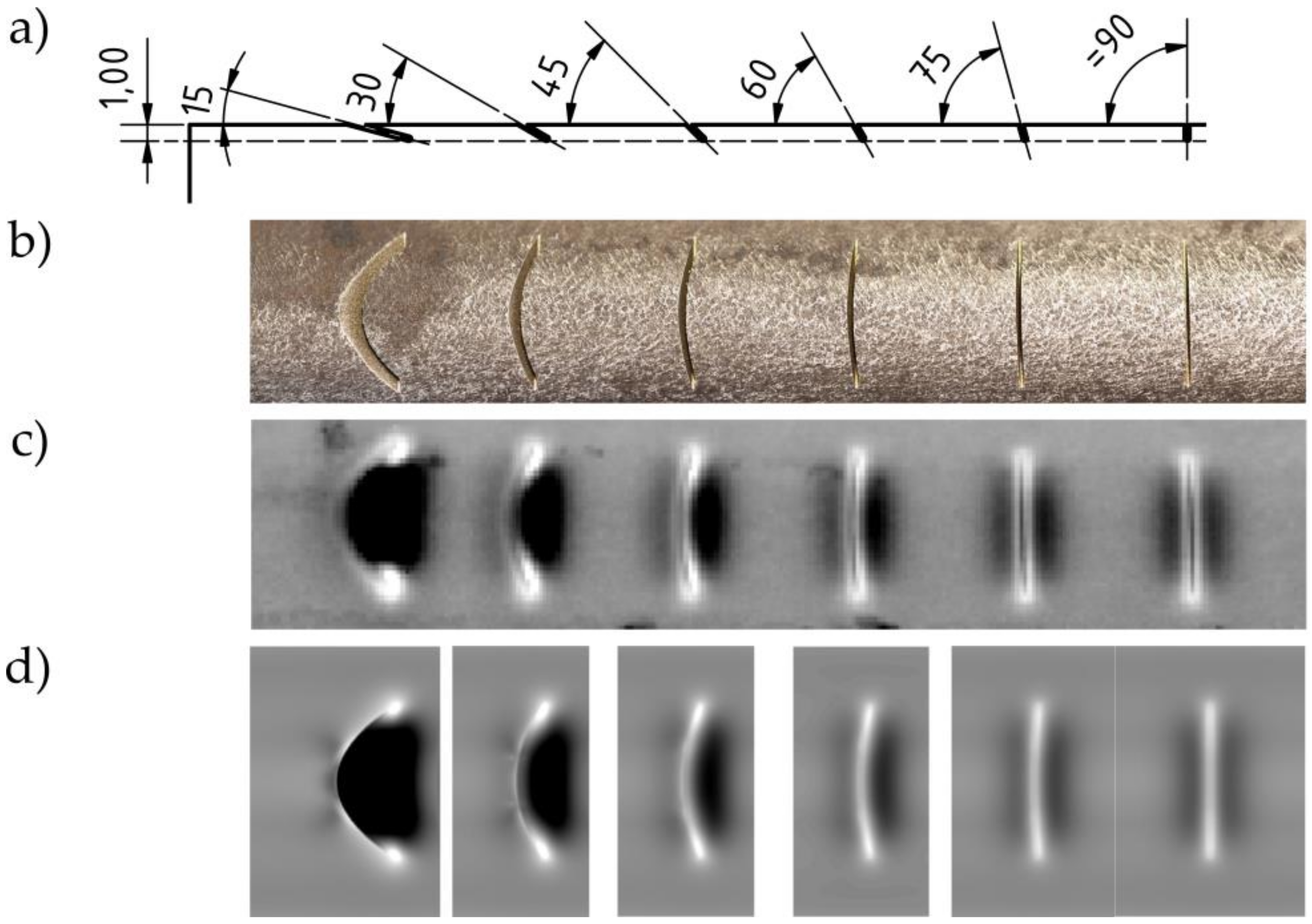
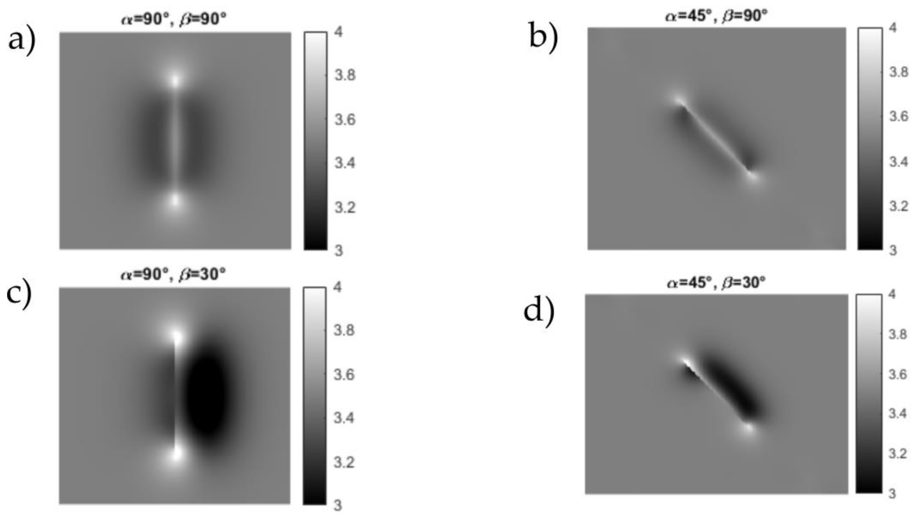
  • The edges of the cuts have higher phase value than the sound part. This is caused by the selective heating of the cuts by the induced eddy currents.
  • At the tips of the cuts an even higher phase value, a kind of ‘hot spot’, can be recognized.
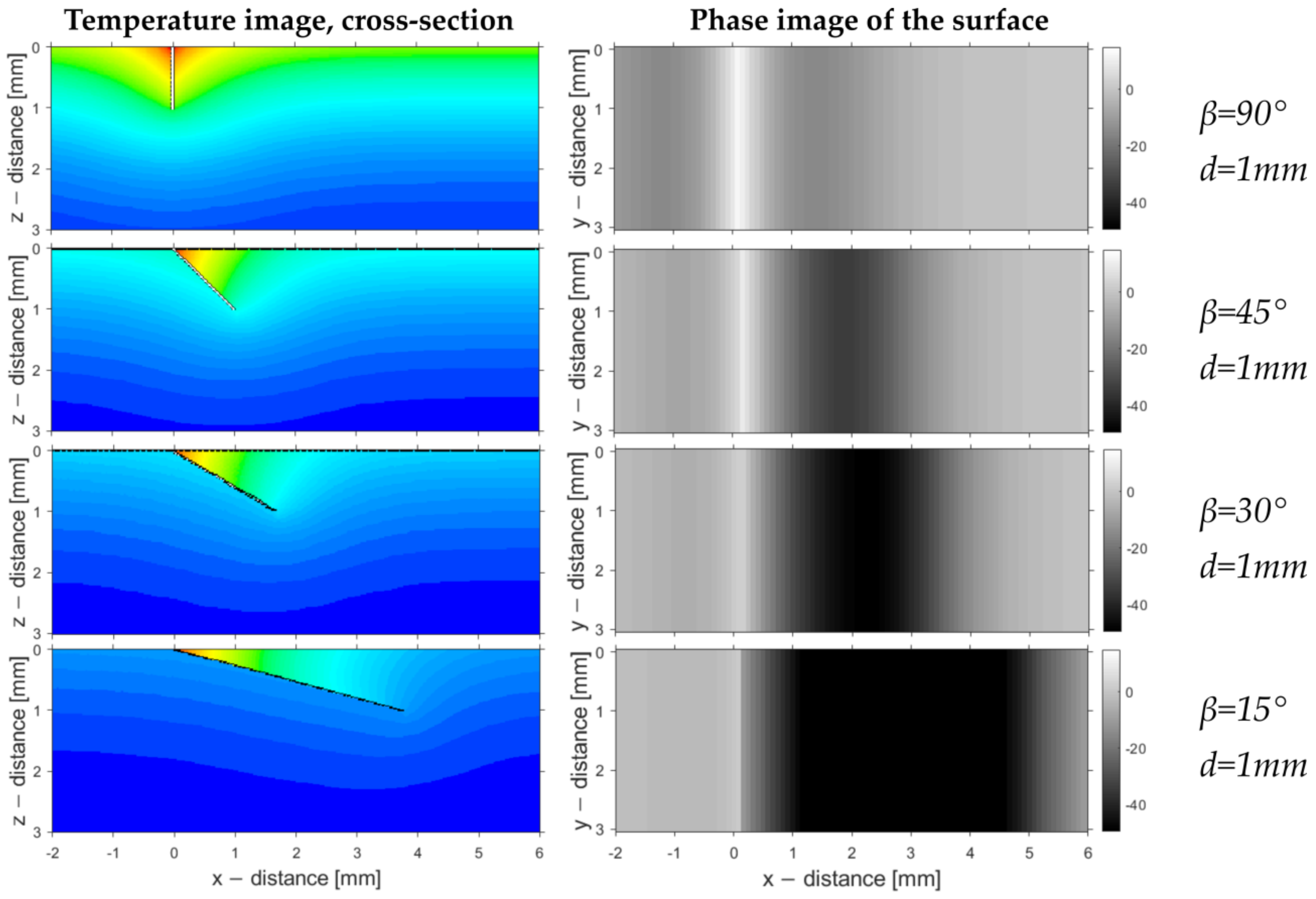
  • At both sides of the cuts darker regions with low phase values can be observed, which are symmetrical. The heat accumulation causes slower cooling rates, which further result in lower phase values [15]. Since the EDM-cuts are perpendicular to the surface, the heat accumulation on both flanks of the cut are identical, resulting a symmetrical pattern.
  • With increasing defect depth, the width of the darker regions and the phase difference also increases. The deeper the crack, the larger the phase contrast around it. Therefore, with a phase image it is possible to estimate the depth of a vertical crack [15].
  • Real cracks have only several µm width, but the EDM-cuts have a width of 0.3 mm, therefore the cut itself is also visible as a dark line in the phase image.
Figure 4d shows the corresponding simulation results for the artificial cracks with depths of between 1.5 and 0.5 mm. The model was used as presented in Figure 3, by varying the crack depth. The width of the cut is not resolved in the simulation, as the goal is to model realistic cracks with very small openings. In this way in the simulation results the dark line along the cut is not visible, but the phase distribution around the crack, caused by the perturbation of the eddy current and heat flow due the crack, is in very good agreement with the experimental results.

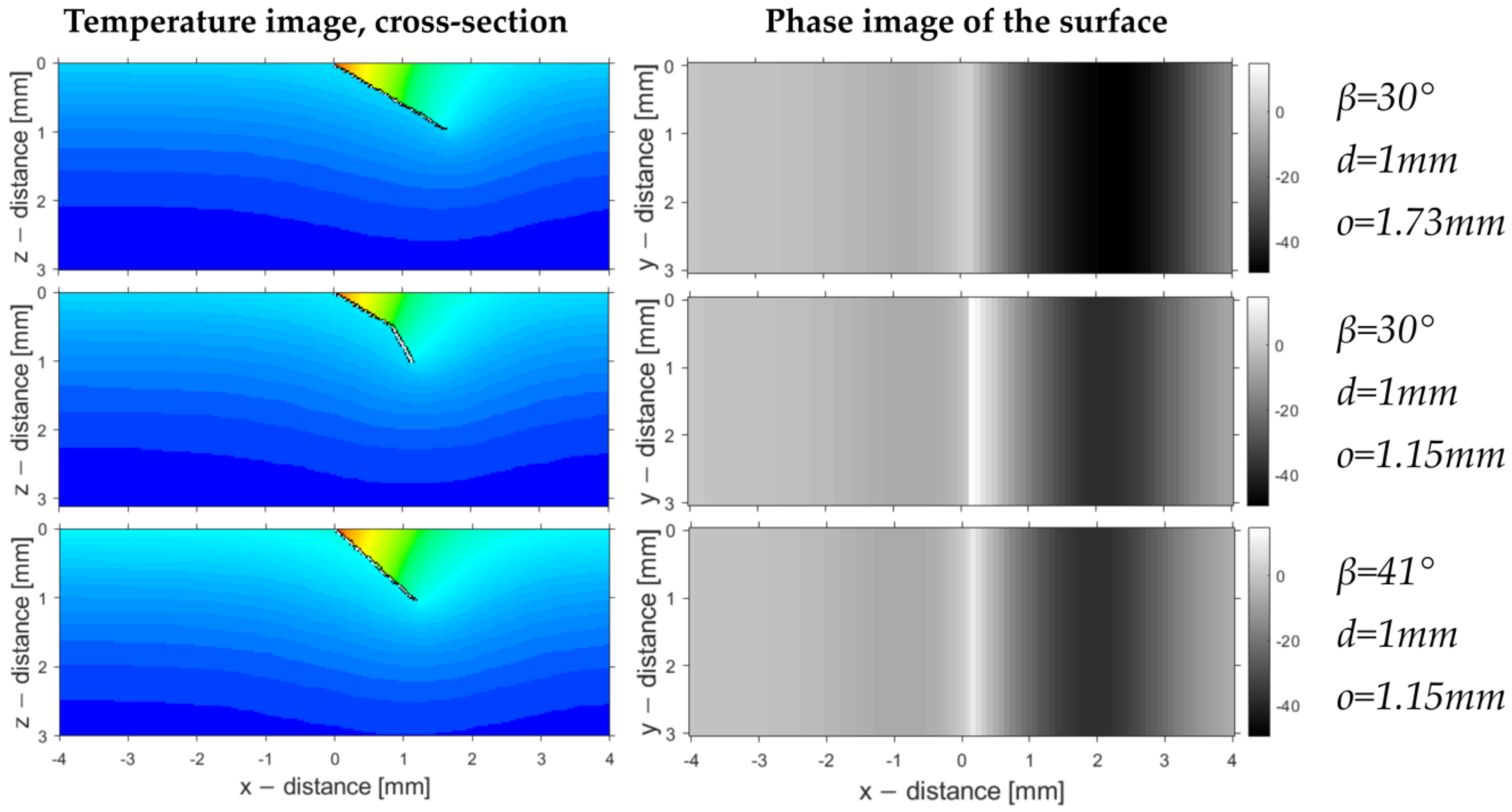
4.2. EDM-Cuts with Different Inclination Angles

Figure 5 shows the results for the other gauge corner on the second side of the reference rail piece RP01. On this side the defect depths of all EDM cuts are identically 1 mm and the inclination angle varies between 90° (perpendicular cut) and 15°, see Figure 5a.
The difference between varying inclination angles in a phase image can be easily recognized in Figure 5c. The EDM cut on the rightest side is perpendicular to the surface and therefore has the same symmetrical feature as described before in Section 4.1. With increasing inclination angle (from right to left) the widths of the darker regions on both sides of the cut become increasingly asymmetrical, as the heat accumulates stronger at the flank with the acute angle. Therefore, the phase image can be used to determine the direction of a crack beneath the surface. Furthermore, estimations of the penetration angle of a crack can be made by using phase images [15]. Figure 5d shows the corresponding simulation results, obtained by a model similar to the one shown in Figure 3. It is noteworthy that the simulation and measurement results agree very well.

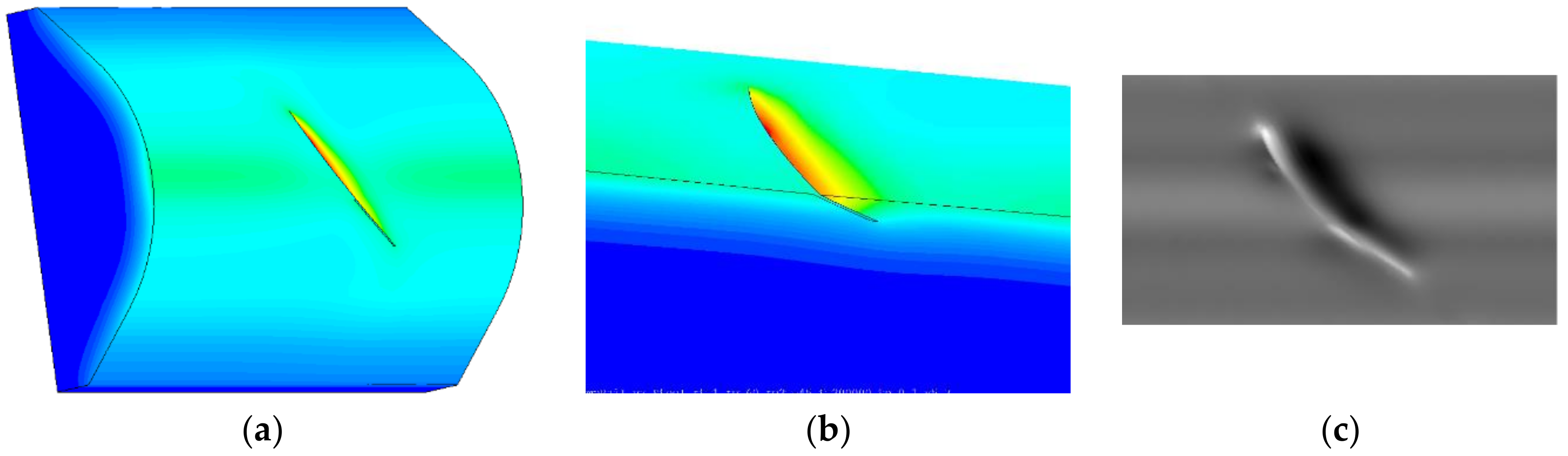
5. Simulations of Realistic Head Checks

In the previous sections it was shown that the experimental and the finite element simulation results correspond very well for the artificial cracks and how the simulation results help to interpret the experimentally achieved phase images. However, these EDM cuts are perpendicular to the rail gauge corner, whereas head checks on rails in service occur at a specific angle. This angle is affected by the local load situation (track curvature and corresponding wheel-rail interaction) and the rail material. Therefore, further simulations were carried out, where the head check shows an angle to gauge line (α) and it has another penetration angle (β) into the material. Figure 6 shows a principle sketch with the definition of the different parameters characterizing the head checks pattern and which were varied in the simulations to investigate their effect on the phase images.
In Figure 7 simulation results are presented for a crack with α = 45° and β = 30°. Figure 7a shows the simulated temperature distribution after 0.1 s inductive heating pulse and in Figure 7b half of the model is presented, whereby the inclination angle and the temperature distribution below the surface are also visible. A phase image is calculated from the simulated temporal change of the temperature, in the same way as it is done for the measurements. This image (Figure 7c) shows a good agreement with the experimental results of head checks.
Further simulations were carried out to investigate how the inclination angle below the surface affects the phase images. In Figure 8 the temperature and phase images are compared for cracks with 1 mm depth but with different angles. The images on the top row show the results for a vertical crack (β = 90°). In this case the temperature and phase distribution are symmetrical around the crack position at x = 0 mm. As the inclination angle decreases, the length of the crack increases to d/sin(β) and the overlapped length o = d/tan(β). In the phase image this overlapping can be easily recognized: due to the small inclination angle the heat is captured for longer in this region, causing a low phase value. It is easy to see that the width of the low phase value region corresponds well to the width of the overlapped region. This gives the possibility of recognizing at the surface of the phase image in which direction the crack is inclined and how wide the overlapped region is.
Figure 9 demonstrates how the angle below the surface (β), the depth and the width of the overlapped region influence the phase image. In the image at the top, the crack is modelled as a straight line, starting with an angle of 30°. In many cases head checks change their direction and, after a small starting angle, penetrate under a larger angle into the rail. The image in the middle of Figure 9 shows such a situation. The starting angle and the depth are the same, as in the case at the top image, but the overlapped region is shorter. This can be also noticed in the phase image, as the region with low phase value is narrower. In the case at the bottom of Figure 9, the crack is again modelled as a straight line, having the same depth and overlapped region as in the middle case, but its starting angle is larger with β = 41°. As the overlapped region is the same is in the middle case, the width of the low phase region is also the same. Due to the slightly larger inclination angle to the surface, the phase value is slightly less at the crack position than in the case in the middle.
In typical head check pattern the cracks are close to each other, therefore the question is how the phase distribution around a crack is influenced by the neighboring cracks. In Figure 10 two situations are compared: in one situation the cracks do not overlap each other in the depth and once in the other situation do. All the cracks have a depth of 1 mm and β = 30°. If the distance between cracks is larger than the overlapped region by a crack, then all the phase values at the crack positions are the same and they are also equal to the phase profile around one single crack (see Figure 10a). If the cracks are closer to each other, then the heat is trapped longer between the cracks than would be the case for one single crack, and the phase value around the crack is less (see Figure 10b). In this way it is possible to tell from the phase image of more parallel cracks, whether they are overlapping each other below the surface or not.
The simulations shown in Figure 8, Figure 9 and Figure 10 were calculated in a 2D model, so the results are valid for long cracks. The head checks have usually a length about 6–10 mm at the surface. In the mid of the crack the phase values are the same as for a long crack, but at the crack tips additional hot spots occur [24]. In Figure 11 the results are presented simulated with a 3D model, where the crack is placed in the middle of a plane surface. For the 6 mm long and 1 mm deep crack the two inclinations angles are varied. If α is 90°, then the line of the crack is perpendicular to the line of the modelled coil (Figure 11a,c), which is lying in the x direction. The angle β is the inclination angle below the surface; if β = 90° the crack is vertical, which means perpendicular to the surface (Figure 11a,b). In Figure 11a the phase pattern is symmetrical, but in Figure 11b the induced eddy currents flow not perpendicular to the crack, but under 45°, therefore the disturbance in the vicinity of the crack is less and also the phase pattern changes along the crack line. Similarly to previous results, the inclination angle below the surface causes an asymmetric phase pattern (Figure 11c,d). The phase pattern of Figure 11d demonstrates the case, which is the most similar one to head checks, as it is presented in the next section.

6. Measurements of Head Checks from Rails in Service

6.1. The Inspected Specimens

Several different rail pieces with head checks have been tested and three representative ones were selected to be presented here. The pieces vary in material as well as how the head checks formed:
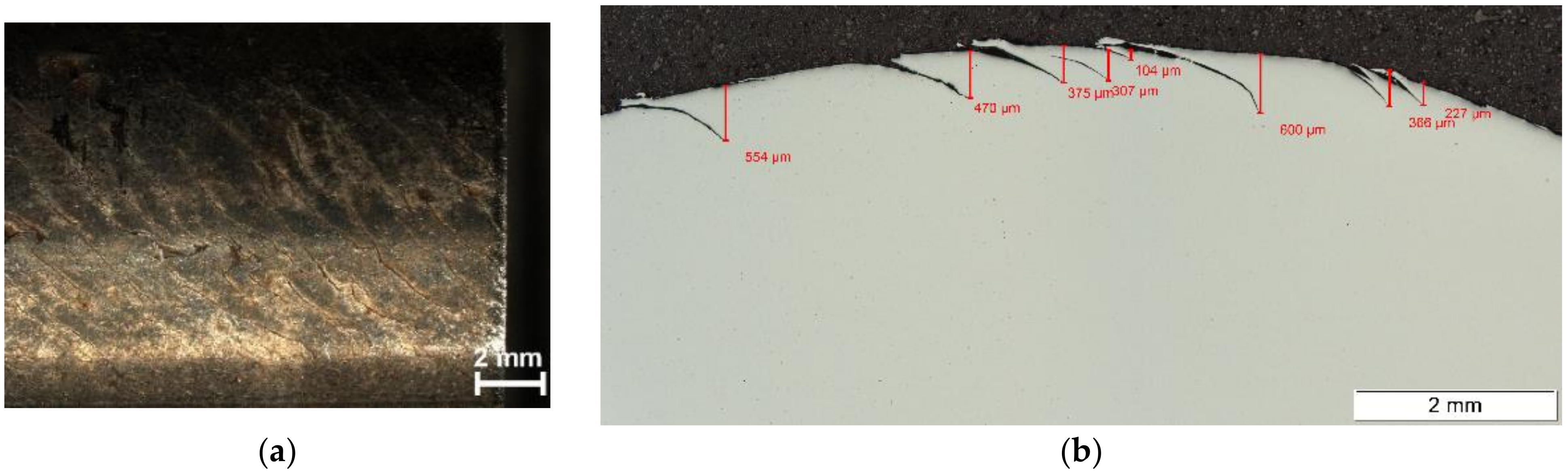
  • RP02: This specimen is a 25 cm long rail head with a R350HT rail grade (see Figure 12). The rail piece was cut out of a demounted rail where head checks occurred during service. Three different micrographs were created from RP02: a cross section of the side view, a vertical cut of the frontal view and a 45° cut. These micrographs revealed head checks with a maximum length of 1803 µm and a maximum penetration depth of 640 µm. Figure 12b shows the side view micrograph image. The travel direction on this rail piece was from left to the right, therefore the head checks incline in a north-west to south-east (NW-SE) direction and the angle α is denoted as a negative angle.
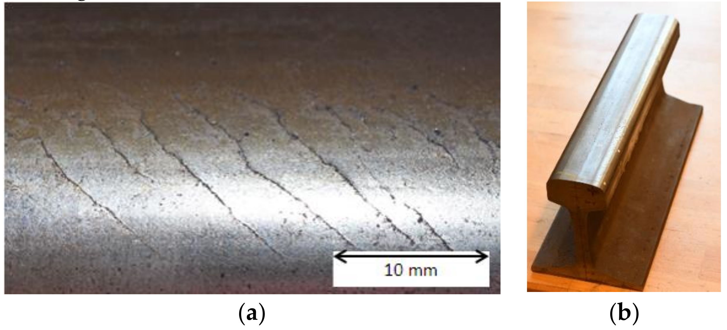
  • RP03: This specimen of rail grade R260 is 45 cm long and it is also a cut-out of a demounted rail. It shows long head checks at the gauge corner and the travel direction was also from left to the right, causing a NW-SE head check orientation (see Figure 13).
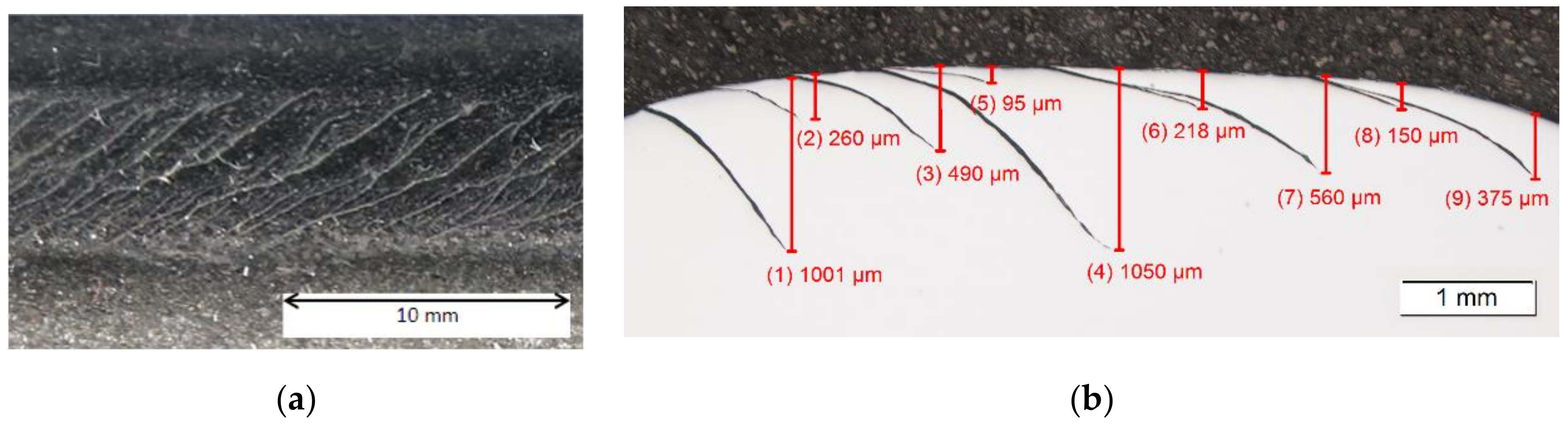
  • RP04: Specimen RP04 is a cut-out piece of a rail with a rail grade R350HT, see Figure 14a. It was tested on the rail-wheel test rig at voestalpine Rail Technology GmbH [2]. The travelling direction was from the right to left, therefore the head checks have an orientation of NE-SW and the inclination angle α has a positive sign. A micrograph of the side view shows head checks with a maximum length of 1675 µm and a maximum penetration depth of 1050 µm, see Figure 14b.

6.2. Characterization of Head Checks

To automatically compute α, the surface angle of head checks, an edge detection algorithm was developed in such a way that the head checks in a phase image are recognized and marked by red lines (see Figure 15). These red lines correspond to the head check lines at the rail surface. The surface angle α is computed as the angle between a horizontal line along the gauge corner and an approximating straight line along the head check, see green line in Figure 15. The mean angle is calculated by averaging for all head checks in the image. The phase image in Figure 15 shows the same part of the rail as the photo in Figure 13a.
The head checks show an approximately 3 mm wide low phase value range at the right side. This is in good agreement with the simulated images of Figure 7c and Figure 11d, therefore the head checks have approximately a 30° inclination angle and a depth around 1 mm.
In Figure 16 two ways of evaluation of the number of head checks as well as their distances on a phase image are shown:
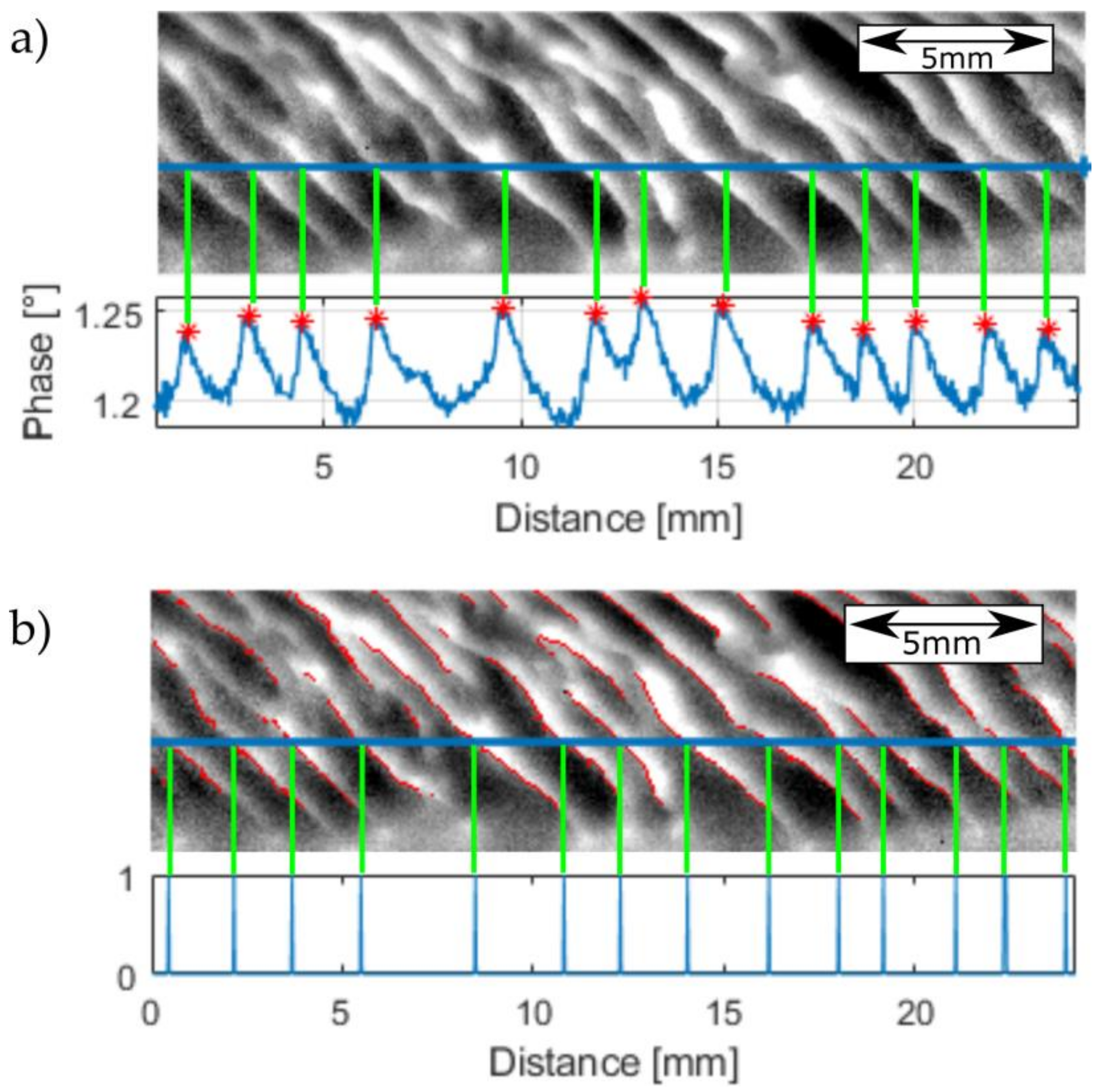
  • In Figure 16a the phase profile along a line over the head checks is evaluated, and the maximum values of the profiles are counted. With the image resolution, given as pixels per mm, the average distance between two head checks is calculated. For the case in Figure 16a it gives 13 head checks for 25 mm, resulting an average distance of 1.9 mm.
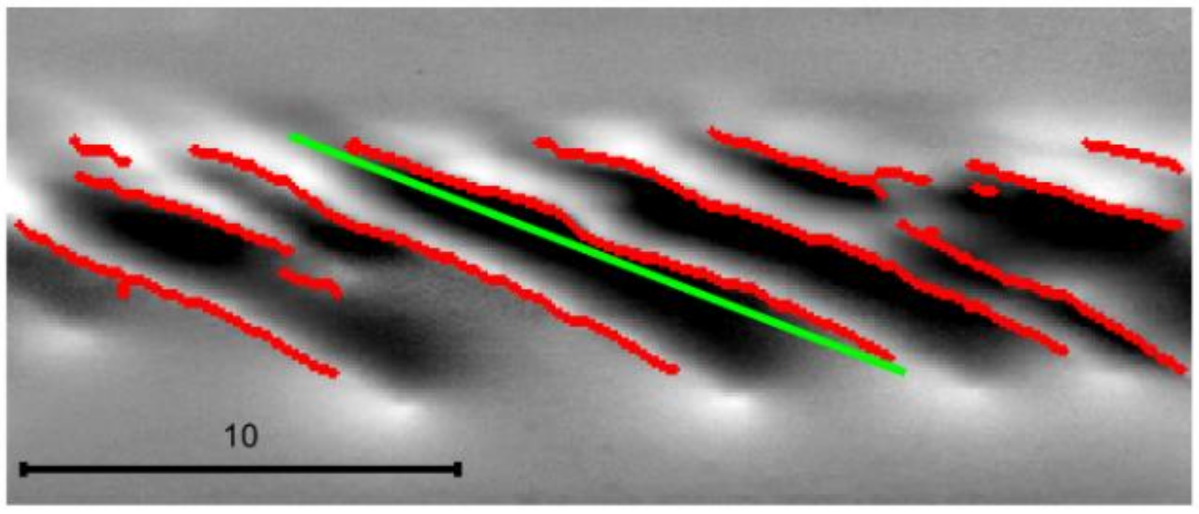
  • Alternatively, the same edge detection algorithm, as in Figure 15, is used to compute the number and the distances of the head checks. Evaluating the results of the edge detection along a straight line produces a plot with peaks where the head checks are located, see Figure 16b. In this case 14 head checks were recognized in the 25 mm distance. As the number of the head checks found along a single line slightly depends on the position of the line, the method was improved in such a way that several lines were taken and an average number of head checks was counted from all of them.

6.3. Inspection of Long Rail Pieces

For the inspection of long rail pieces two different kinds of measurement were carried out and compared, a ‘stop-and-go’ measurement and a scanning technique:
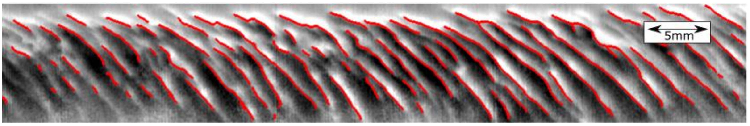
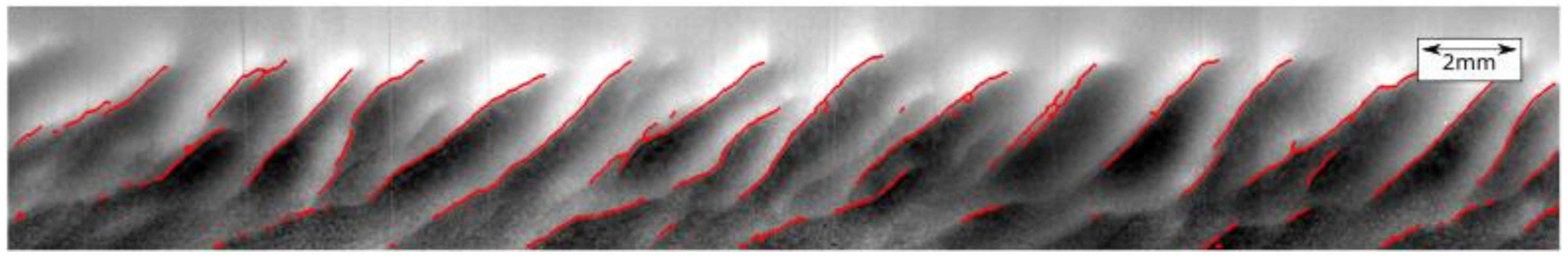
  • In a ‘stop-and-go’ procedure a linear table moves the rail for a certain distance between two static measurements. In one measurement a rail piece of about 25 cm is inspected, and each static measurement is separately evaluated to a phase image. For the calculation of the panoramic view of the entire rail piece, in first step a rectification of the phase images is necessary. This means that perspectivity and distortion due to the IR camera optics has to be eliminated. This was carried by usage of a calibration object, for which a chessboard similar pattern was taken. This technique will be described in more detail in a separate publication. Figure 17 shows a panorama image, which was created out of 5 overlapping static measurements for RP02. One static measurement covers an area of 440 × 1273 pixels with a resolution of 45.225 pixels/mm. Since the size of each image and the movement of the linear table is known, the images can be shifted horizontally to their approximate position. In the next step, the exact position was calculated by means of phase correlation in the overlapping area of two consecutive images, and the images were merged to form one panorama image. This step was repeated for each consecutive images to create one panorama image from the 5 separate measurements. As in this figure the cracks are not well visible due to the limited pixel resolution of a print-out, we have created a video, which is available as additional online material in Supplementary Materials to this paper.
The previously presented characterization technique of the head checks can also be applied to the panorama images. Figure 18 demonstrates this. This was done for the same image as in Figure 17, but here only a shorter part is shown, as the head checks can be better seen in this way.
Figure 19 shows the same edge detection technique applied to the rail piece RP04. It is of note that the head checks on this rail piece have another orientation along NE-SW, as the travel direction was from the right to the left.
  • In the second measurement technique the rail piece is continuously moved by a linear table and it is ‘scanned’ in the region heated by the induction coil. The top section of the rail is heated with a single thread coil and the IR camera is positioned in a way that the areas before and after the heated area, as well as the area under the coil, are recorded. The recorded IR sequence is re-ordered in such a way that each location of the rail has its temperature value assigned according its distance behind the heating position [25]. Likewise, in this case a rectification of the recorded sequence is necessary to eliminate the perspectivity in the image created by the IR camera. The transformed and re-ordered sequence shows a heating process which is similar to a static measurement and an evaluation to a phase image is possible. In Figure 20 the resulting phase image of such a scan can be seen, performed on RP02. Although the scan was carried out over the whole length of 25 cm of the rail, only 10 cm of the phase image is shown in Figure 20, due to the otherwise too large size of the image.
Comparing the two measurement techniques, the following points can be stated:
  • With the ‘stop-and-go’ method the phase images have better contrast than with the scanning technique, and the head checks can be better located and characterized in higher quality.
  • The ‘stop-and-go’ inspection method is slower and more difficult to realize for inspection of long rails than the scanning method.
Therefore, further investigations are planned to improve the evaluation of the scanning method to create images with similar quality as the ‘stop-and-go’ technique.

6.4. Characterization of the Rail Pieces

With the methods discussed in the previous sections, the average inclination angle distance as well as the average head check length were determined by the novel image processing algorithm. Since the panorama images are rectified, the calculated angles and lengths are not distorted any more by the camera optic and by the curvature of the rail. Table 1 summarizes the results for the 3 presented rail pieces. It is of note that α is negative for RP02 and for RP03, as the head checks have an orientation of NW-SE, and on the other hand RP04 has a positive angle due to the NE-SW orientation.

7. Detecting Squats

Additionally to head checks there are also other types of defects which may occur on rails. Another typical defect, called a squat, usually occurs on straight tracks; this is the opposite of head checks, which usually arise in the curves. Squats occur on the rail crown and along the rail. In a critical stage the crack has a small inclination angle below the surface, and it can cause breakouts on the rail. This kind of defect can be also very well detected by inductive thermography, as is shown in Figure 21a. The short, shallow cracks along the line can be the starting point for the later critical damage caused by squats. The two patterns with half-elliptical shape and low phase value are caused by the squats, by cracks in a half-elliptical shape. Figure 21b shows a close-up photo of the right squat. Further investigations using this technique to elucidate the development of squats are planned.

8. Discussion and Conclusions

Inductive thermography is an excellent non-destructive testing method for localizing surface defects in metallic materials in a contact-free and quick way. Especially in the case of ferro-magnetic materials, inductive heating is very efficient and a short heating pulse of 0.1–0.3 s is enough to achieve 1–2 °C of temperature increase at the surface during the heating, which allows the detection of irregularities with an IR camera. A further advantage of the method is that it not only shows the cracks at the surface, but it also gives an impression of how the cracks lie below the surface. The recorded IR sequence is evaluated in one phase image, reducing the negative effects of inhomogeneous heating and inhomogeneous surface properties, and resulting in an image with very good quality.
Head checks on railway rails can cause catastrophic events if they are not detected in time. Nowadays, eddy current testing and ultrasound testing are usually used to inspect the rails. Inductive thermography has great potential as non-destructive testing method to inspect the rails, but the technique is not yet used in the field, only in the laboratory. We have inspected several different railway rails and developed an image processing tool for characterizing head checks. Two different kinds of measurement method were used to inspect long tracks: ‘stop-and-go’ and the scanning technique. The first one gives better results with higher contrast, but the second one is more practicable. Therefore, further research work is planned to improve the quality of the scanning technique to obtain the same image quality as the ‘stop-and-go’ method.

Supplementary Materials

The following are available online at https://www.mdpi.com/2076-3417/11/3/1003/s1, Video S1: Panorama View.

Author Contributions

C.T. has performed the experiments, evaluated the images, calculated the rectification and the scanning technique. B.O.-T. has done the finite element simulations, developed the theory behind the software and written the main part of the software, and she supervised C.T. by his work. S.E. has provided the rail test specimens, organized the artificial crack arrangements and contributed to the text via the section on head check development and proof reading. All authors have read and agreed to the published version of the manuscript.

Funding

The authors gratefully acknowledge the financial support under the scope of the COMET program within the K2 Center “Integrated Computational Material, Process and Product Engineering (IC-MPPE)” (Project No 859480). This program is supported by the Austrian Federal Ministries for Climate Action, Environment, Energy, Mobility, Innovation and Technology (BMK) and for Digital and Economic Affairs (BMDW), represented by the Austrian research funding association (FFG), and the federal states of Styria, Upper Austria and Tyrol.

Institutional Review Board Statement

Not applicable.

Informed Consent Statement

Not applicable.

Acknowledgments

The authors gratefully acknowledge the support from voestalpine Rail Technology GmbH, especially D. Künstner and S. Scheriau. Furthermore.

Conflicts of Interest

The authors declare no conflict of interest.

References

  1. Eadie, D.T.; Elvidge, D.; Oldknow, K.; Stock, R.; Pointner, P.; Kalousek, J.; Klauser, P. The effects of top of rail friction modifier on wear and rolling contact fatigue: Full-scale rail–wheel test rig evaluation, analysis and modelling. Wear 2008, 265, 1222–1230. [Google Scholar] [CrossRef]
  2. Simon, S.; Saulot, A.; Dayot, C.; Quost, X.; Berthier, Y. Tribological characterization of rail squat defects. Wear 2013, 297, 926–942. [Google Scholar] [CrossRef]
  3. Daves, W.; Kráčalík, M.; Scheriau, S. Analysis of crack growth under rolling-sliding contact. Int. J. Fatigue 2019, 121, 63–72. [Google Scholar] [CrossRef]
  4. Stock, R.; Kubin, W.; Daves, W.; Six, K. Advanced maintenance strategies for improved squat mitigation. Wear 2019, 436, 203034. [Google Scholar] [CrossRef]
  5. Zhou, Y.; Zheng, X.; Jiang, J.; Kuang, D. Modeling of rail head checks by X-ray computed tomography scan technology. Int. J. Fatigue 2017, 100, 21–31. [Google Scholar] [CrossRef]
  6. Railhead Damage, Squats. Available online: http://railmeasurement.com/railhead-damage/discrete-defects/squats (accessed on 18 June 2019).
  7. Magel, E.E. Rolling Contact Fatigue: A Comprehensive Review; U.S. Department of Transportation, Office of Railroad: Washington, DC, USA, 2011.
  8. Fan, Y.; Dixon, S.; Edwards, R.S.; Jian, X. Ultrasonic surface wave propagation and interaction with surface defects on rail track head. NDT&E Int. 2007, 40, 471–477. [Google Scholar]
  9. Cavuto, A.; Martarelli, M.; Pandarese, G.; Revel, G.; Tomasini, E. Experimental investigation by Laser Ultrasonics for train wheelset flaw detection. J. Phys. Conf. Ser. 2018, 1149, 012015. [Google Scholar] [CrossRef]
  10. Montinaro, N.; Epasto, G.; Cerniglia, D.; Guglielmino, E. Laser ultrasonics for defect evaluation on coated railway axles. NDT E Int. 2020, 116, 102321. [Google Scholar] [CrossRef]
  11. Wilson, J.; Tian, G.; Mukriz, I.; Almond, D. PEC thermography for imaging multiple cracks from rolling contact fatigue. NDT&E Int. 2011, 44, 505–512. [Google Scholar]
  12. Netzelmann, U.; Walle, G.; Ehlen, A.; Lugin, S.; Finckbohner, M.; Bessert, S. NDT of Railway Components Using Induction Thermography. AIP Conf. Proc. 2016, 1706, 150001. [Google Scholar]
  13. Vaibhav, T.; Balasubramaniam, K.; Thomas, R.; Bose, A.C. Eddy current Thermography for rail inspection. Proc. QIRT Conf. 2016. [Google Scholar] [CrossRef]
  14. Tuschl, C.; Oswald-Tranta, B.; Künstner, D.; Eck, S. Schienenprüfung mittels induktiv angeregter Thermografie. In Proceedings of the DACH Conference, Friedrichshafen, Germany, 27–29 May 2019. [Google Scholar]
  15. Oswald-Tranta, B. Induction thermography for surface crack detection and depth determination. Appl. Sci. 2018, 8, 257. [Google Scholar] [CrossRef] [Green Version]
  16. Maldague, X. Infrared and Thermal Testing. In Nondestructive Testing Handbook; ASNT: Columbus, OH, USA, 2001; Volume 3. [Google Scholar]
  17. Netzelmann, U.; Walle, G.; Lugin, S.; Ehlen, A.; Bessert, S.; Valeske, B. Induction thermography: Principle, applications and first steps towards standardisation. Quant. Infrared Thermogr. J. 2016, 13, 170–181. [Google Scholar] [CrossRef]
  18. Vrana, J.; Goldammer, M.; Baumann, J.; Rothenfusser, M.; Arnold, W. Mechanism and models for crack detection with induction thermography. Proc. AIP Conf. 2008, 975, 475–482. [Google Scholar]
  19. Srajbr, C. Induction excited thermography in industrial applications. In Proceedings of the 19th World Conference on Non-Destructive Testing, Munich, Germany, 13–17 June 2016. [Google Scholar]
  20. DIN 54183:2018-02, Non-Destructive Testing-Thermographic Testing- Eddy-Current Excited Thermography. Available online: https://www.din.de (accessed on 1 January 2018).
  21. Oswald-Tranta, B. Time-resolved evaluation of inductive pulse heating measurements. Quant. InfraRed Thermogr. J. 2009, 6, 3–19. [Google Scholar] [CrossRef]
  22. Oswald-Tranta, B. Lock-in inductive thermography for surface crack detection in different metals. QIRT J. 2019, 16, 276–300. [Google Scholar] [CrossRef]
  23. ANSYS, Inc. Available online: http://www.ansys.com (accessed on 1 January 2018).
  24. Oswald-Tranta, B.; Tuschl, C. Detection of short fatigue cracks by inductive thermography. In Proceedings of the 15th QIRT Conference, Porto, Portugal, 21 September–31 October 2020. [Google Scholar]
  25. Oswald-Tranta, B.; Sorger, M. Scanning pulse phase thermography with line heating. QIRT J. 2012, 9, 103–122. [Google Scholar] [CrossRef]
Figure 1. The setup for measuring railway rails in the laboratory.
Applsci 11 01003 g001
Figure 2. a: Top image: thermogram after an inductive heating pulse of 0.1 s; two points were marked: (a) point on a crack position, (b) point on sound surface; bottom image: phase image for the same measurement; b: temperature vs. time diagram of the heating and cool-down for the two marked points in (a).
Applsci 11 01003 g002
Figure 3. Left side: geometrical model of the rail in the head check region; mid: temperature distribution after 0.1 s inductive heating pulse; right side: half of the same model in order to show the temperature distribution below the surface.
Applsci 11 01003 g003
Figure 4. (a) CAD drawing of the electrical discharge-machining (EDM) cuts; (b) photo of the rail piece with the vertical EDM-cuts at the gauge corner; (c) phase image of the vertical EDM-cuts after 0.1 s inductive heating pulse; (d) simulation results for 5 of the 7 artificial cracks.
Applsci 11 01003 g004
Figure 5. (a) CAD drawing of the EDM-cuts; (b) photo of EDM-cuts with different penetration angles; (c) phase image of EDM-cuts after 0.1 s inductive heating pulse; (d) simulation results of the slanted artificial cracks.
Applsci 11 01003 g005
Figure 6. The definition of the characteristic parameters at the surface (a) and in cross-section (b): α: inclination angle at the surface to the gauge corner; l: length of the head check at the surface; c: distance of the head checks; β: inclination angle below the surface; d: depth; o: width of overlapped region.
Applsci 11 01003 g006
Figure 7. The simulated temperature results for one crack at the gauge corner after 0.1 s inductive heating pulse; (a) the whole 3D model; (b) half of the model; (c) calculated phase image from the surface temperature.
Applsci 11 01003 g007
Figure 8. The simulation results for cracks with d = 1 mm depth. The inclination angles are varied from β = 90° to 15°. The left column of images shows the temperature after 0.1 s inductive heating, and the right one the corresponding phase images.
Applsci 11 01003 g008
Figure 9. The simulation results for cracks with d = 1 mm depth, investigating the effect of the region width, which is overlapped by the crack below the surface.
Applsci 11 01003 g009
Figure 10. Simulation results for three cracks with d = 1 mm depth and inclination angle of β = 30°. In figures (a) and (b) at the top: temperature distribution in the cross-section; mid: phase distribution at the surface; bottom: phase profile through the cracks at the surface along the x axis. (a): distance between the cracks is 2 mm, therefore they do not overlap each other below the surface; (b): distance of the cracks is 1 mm and overlapping each other in the depth.
Applsci 11 01003 g010
Figure 11. Simulated phase images for cracks with d = 1 mm depth and l = 6 mm length at the surface with different inclination angles at and below the surface. (a): the crack is perpendicular to the gauge corner (α = 90°) and it is perpendicular to the surface (β = 90°); (b): the crack has an angle of 45° (α) to the gauge corner and it is perpendicular to the surface (β = 90°); (c): the crack is perpendicular to the gauge corner (α = 90°) and it has an angle of 30° to the surface (β); (d): the crack has an angle of 45° (α) to the gauge corner and it has an angle of 30° to the surface (β).
Applsci 11 01003 g011
Figure 12. (a) A photo of the head checks on RP02; (b) the head checks in cross section side view micrograph of RP02.
Applsci 11 01003 g012
Figure 13. (a) A close up of the head checks on RP03; (b) a photo of RP03.
Applsci 11 01003 g013
Figure 14. (a) A photo of the head checks on RP04; (b) a micrograph of head checks on RP04.
Applsci 11 01003 g014
Figure 15. Phase image of RP03 with edge detection of head checks (heating pulse duration: 0.1 s).
Applsci 11 01003 g015
Figure 16. Two options for counting head checks for RP02; (a) distances of head checks with profile of the phase image; (b) distances of head checks with edge detection.
Applsci 11 01003 g016
Figure 17. A panorama image from five measurements of RP02 (heating pulse duration: 0.3 s).
Applsci 11 01003 g017
Figure 18. A shorter part of the panorama image in Figure 17, with markings for the located head checks.
Applsci 11 01003 g018
Figure 19. Part of a panorama image for RP04, with markings for the located head checks.
Applsci 11 01003 g019
Figure 20. A phase image of the scan of RP02; speed of motion is 10 cm/s.
Applsci 11 01003 g020
Figure 21. (a): Phase image of squat defects measured with inductive thermography; (b): close-up photo of the right squat.
Applsci 11 01003 g021
Table 1. The results from the three different pieces of rail.
Average Surface Angle (α)Average Distance
(c) [mm]
Average Length
(l) [mm]
RP02−40°2.5417.1
RP03−42°5.2721.8
RP0436°1.79.2
Publisher’s Note: MDPI stays neutral with regard to jurisdictional claims in published maps and institutional affiliations.

