Improvement of Wheat Grain Yield Prediction Model Performance Based on Stacking Technique

Abstract

Crop growth and development is a dynamic and complex process, and the essence of yield formation is the continuous accumulation of photosynthetic products from multiple fertility stages. In this study, a new stacking method for integrating multiple growth stages information was proposed to improve the performance of the winter wheat grain yield (GY) prediction model. For this purpose, crop canopy hyperspectral reflectance and leaf area index (LAI) data were obtained at the jointing, flagging, anthesis and grain filling stages. In this case, 15 vegetation indices and LAI were used as input features of the elastic network to construct GY prediction models for single growth stage. Based on Stacking technique, the GY prediction results of four single growth stages were integrated to construct the ensemble learning framework. The results showed that vegetation indices coupled LAI could effectively overcome the spectral saturation phenomenon, the validated R² of each growth stage was improved by 10%, 22.5%, 3.6% and 10%, respectively. The stacking method provided more stable information with higher prediction accuracy than the individual fertility results (R² = 0.74), and the R² of the model validation phase improved by 236%, 51%, 27.6%, and 12.1%, respectively. The study can provide a reference for GY prediction of other crops.

1. Introduction

Wheat is one of the most widely cultivated food crops in the world, with China ranking first in terms of yield and sales [1]. Therefore, a timely and accurate prediction of grain yield (GY) can not only help guide agricultural production management and assist relevant government departments to formulate scientific food policies, but also has significance for mitigating climate risks, ensuring national food security and economic stability [2,3,4,5,6,7]. The essence of the formation of the yield is the accumulation of dry matter produced by photosynthesis in different growth stages. The level of GY is influenced by complex factors such as light, soil, moisture, and atmosphere, which poses a great challenge to the accurate prediction of GY [8]. The conventional GY measurement method is not only expensive and less efficient, but also harmful to crops, making it unsuitable for large-areas crop yield estimation [9,10]. In recent decades, remote sensing technology has been successfully applied to crop growth monitoring through satellite platforms, manned airborne platforms, and ground spectral equipment [11]. However, several limitations such as deficient temporal-spatial resolution and cloud cover contamination restrain the application of satellite-based platforms [12]. In comparison, near-ground hyperspectral remote sensing data is not only cost-effective, but also has narrow band, strong continuity, and large spectral information contents [13]. In recent years, scholars at home and abroad have carried out research and made progress in yield estimation of various crops using remote sensing technology [14,15,16]. To the best of our knowledge, most current studies construct GY prediction models by using a single index such as spectral reflectance, spectral index, or vegetation index. However, as the plants grow, spectral saturation occurs when the crop coverage is high, making it difficult to continue improving GY prediction accuracy.

The essence of crop yield formation is the continuous accumulation of dry matter produced by photosynthesis in the plant body [17,18]. It was found that LAI determines many biophysical processes, such as photosynthesis, respiration, and transpiration in crops [19,20]. LAI is used as a common monitoring variable during crop growth and development and has a close relationship with final crop yield [21]. For example, Li et al. [22] used UAV-based hyperspectral remote sensing data to evaluate correlations between soybean yield and physiological and ecological parameters such as plant height, LAI, fresh biomass, and dry biomass, and identified LAI and fresh biomass as key indicators of soybean yield. Dente et al. [23] proved that LAI was closely related to GY by studying the influence of LAI at different growth stages of wheat on GY estimation and concluded that LAI can be used as an important index for GY estimation. Delécolle et al. [24] used remote sensing inversion data on the LAI as the input parameter of an output estimation model to improve the accuracy of the output estimation. Based on this, an important objective of this study is to use the winter wheat canopy structure parameter LAI coupled with vegetation indices as input features for yield prediction, in order to effectively overcome the canopy spectral saturation phenomenon.

The level of GY mainly depends on the number of ears, grains, and thousand seed weight of the crop [25]. During the growth stage of wheat from the jointing stage to the flag-raising stage, the LAI increases quickly, which is more conducive to accelerating the photosynthesis of plants. This period plays a decisive role in the number of ears of wheat. The number of grains in wheat mainly depends on the intensity of the photosynthesis from the flagging stage to the anthesis stage. In this growth period, there is a transition from vegetative growth to reproductive growth, and the nutrient transfers from the leaves to the ear, so it is the key period of grain formation and accumulation. After the anthesis stage, the number of grains per panicle is determined. The thousand seed weight of wheat is mainly determined by the intensity of photosynthesis and the rate of energy transfer from the anthesis to the grain filling stage [26,27]. Therefore, the physiology, shape, and structure of the crop vary throughout the growth cycle from germination, flowering, and fruiting to senescence and death, and the formation of GY occurs sequentially and overlappingly at different growth stages [28]. A study has shown that each key growth period of crop is closely related to the formation of the final GY [4]. Most existing studies considered the grain filling stage as the key stage of GY formation; therefore, it was considered to have the best prediction accuracy in many studies [29]. Hernandez et al. [30] reached a similar conclusion in that a penalized ridge regression model constructed using spectral reflectance data at the anthesis or grain filling stages could effectively predict GY at different water levels. However, the GY prediction model constructed using only a single critical growth stage will lose part of GY correlation information, and the prediction results may vary with the changes in the vegetation types, growth stages, and environmental conditions. Moreover, the robustness of the model is not strong, and the generalization ability is weak [31,32]. Based on this, many researchers have proposed multitemporal vegetation index-based GY prediction models to improve the accuracy and universality of model prediction. For example, Patel et al. [33] used multitemporal Terra/MODIS satellite data to simulate GY in the west of Uttar Pradesh, India. Li et al. [34] used the support vector regression method to construct a GY prediction model based on the normalized vegetation index obtained from multitemporal Landsat TM images, which effectively improved the prediction accuracy. Li et al. [35] used a large regional remote sensing GY estimation model based on multifertility MODIS-NDVI data and obtained a higher estimation accuracy than the single-fertility GY prediction model. Ghizlane et al. [36] obtained multispectral data of the four key growth periods of wheat based on the UAV remote sensing platform and estimated GY using the method of random forest combined with the vegetation index. To the best of our knowledge, there are no studies related to the ensemble of ground spectral data and LAI data from multiple growth stages of crops for yield prediction. Therefore, it is important to find a method that can combine the advantages of multiple growth stages to achieve an improved prediction accuracy and robustness for grain yield prediction.

As an important part of ensemble learning, the stacking method trains a secondary model through “learning method”, which is used to combine other primary models. Most existing studies applied this method to heterogeneous models to integrate and improve the final prediction accuracy of the model using the differences between the primary models [37]. Currently, this method has been applied to the prediction of plant photosynthesis capacity, map synthesis, and forest coverage monitoring [38,39,40]. Considering the heterogeneity of the canopy spectral information in the different growth stages of crops, multiple key growth stages related to GY formation were selected, and the integration of hyperspectral data and phenotypic data of the multiple growth stages based on the stacking method was studied. This was helpful to improve the estimation accuracy and generalization ability of the GY prediction model.

In recent years, machine-learning techniques using spectral reflectance data as input to build predictive models for plant traits have been employed and have shown improved prediction accuracy and robustness [41]. The elastic net algorithm is a type of neural network first proposed by Durbin and Willshaw [42]. Recently, the elastic network algorithm has been proven to achieve excellent results in machine learning, which can effectively avoid over fitting of the model prediction results due to small sample size and high dimension. For example, based on the elastic network regression model, Wang et al. [43] constructed the transmission and distribution cost allocation model of a power grid project to realize a reasonable allocation of operation and maintenance cost. Chen et al. [44] proposed a dam deformation prediction model based on the extreme learning machine and elastic network. The elastic network algorithm effectively alleviated the over fitting phenomenon, which remains challenging for the extreme learning machine, and the prediction results showed better stability. These results indicate that elastic networks can be used to solve regression problems.

To our knowledge, no studies have applied the strategy of combining the ENET algorithm and stacking techniques to stack LAI and hyperspectral data from multiple growth cycles to construct an ensemble learning framework for GY prediction. The main objectives of this study are as follows: (1) To assess the ability of winter wheat canopy hyperspectral vegetation indices and LAI to be used for grain yield prediction based on the ENET algorithm; (2) to study the effect of Stacking technology in improving the accuracy of grain yield prediction based on ensemble learning; (3) to analyze the influence of each individual growth stage on the development of an accurate integrated learning model. To achieve these goals, the correlations between 15 vegetation indices and LAI from four growth stages and yield were analyzed. Then, yield prediction models for individual growth stage of winter wheat were constructed based on the ENET algorithm in two cases of vegetation indices without or with coupled LAI, respectively. Finally, stacking techniques were used to integrate the yield prediction capabilities in the four growth stages, develop an ensemble learning framework to improve the robustness of the model, and analyze the weights attributed to each growth stage based on the prediction results.

2. Materials and Methods

2.1. Experiment Location and Research Material

Field trials were conducted in Yongxingtun village, Shanyang District, Jiaozuo City, Henan Province, China, during two cropping seasons in 2016–2017 and 2017–2018. Figure 1 showed the specific location of the study area. The experimental area was 110 m in length from east to west and 38 m in length from north to south, with each plot measuring 6 m × 8 m. There were 48 plots, 16 treatments, and three replications. The orthogonal experiment was conducted with different amounts of nitrogen fertilizer, different moisture contents, and different crop varieties (

Table A1. Combination of different treatments.

N2—W1—P2	N1—W1—P1	N4—W1—P2	N3—W1—P1
N4—W2—P2	N3—W2—P1	N2—W2—P2	N1—W2—P1
N3—W2—P2	N4—W2—P1	N1—W2—P2	N2—W2—P1
N1—W3—P2	N2—W3—P1	N3—W3—P2	N4—W3—P1

Variety treatment—P₁: Jing 9843; P₂: Zhong Mai 175. Nitrogen treatment—N₁: 0 kg/hm²; N₂: 195 kg/hm²; N₃: 390 kg/hm²; N₄: 585 kg/hm². Moisture treatment—W₁: no irrigation; W₂: irrigation water 192 mm; W₃: irrigation water 384 mm.

). Four levels of N fertilizer were set: 0, 0.0195, 0.0390, and 0.0585 kg/m², respectively; three levels of water irrigation were set: rainfed (W1, no irrigation), normal water (W2, irrigation water 192 mm), and twice normal water (W3, irrigation water 384 mm); there are two crop varieties: Jing 9843 (J9843) and Zhong Mai 175 (ZM175). The experimental design scheme was described in Figure A1.

Figure 2 showed the general framework of this paper, which consists of four main parts. (1) Data acquisition: simultaneous acquisition of winter wheat canopy hyperspectral data and LAI data at the jointing, flagging, anthesis, and grain filling stages, and acquiring the GY data during the winter wheat harvest period; (2) Data processing: pre-processing and statistical analysis of measured data using ViewSpecPro, SPSS, Origin and Excel, and construction of various vegetation indices; (3) Data analysis: to explore the relationship between GY and LAI and vegetation indices, respectively, through correlation analysis; (4) Model framework construction: first, 15 vegetation indices and LAI coupled vegetation indices were used as input features for the ENET model to construct individual growth stages GY prediction models. Subsequently, based on the Stacking technology, the GY prediction results of the different growth stages were stacked to construct the GY prediction model that integrates multiple growth stages. Finally, the accuracy of each model was evaluated to screen the optimal model for winter wheat GY prediction.

2.2. Data Collection and Processing

2.2.1. ASD Canopy Hyperspectral Data

The canopy spectral reflectance of winter wheat measurements was performed using an ASD FieldSpec spectroradiometer. The spectral range of the ground object spectrometer was 350–2500 nm, the spectral sampling interval was 1.4 nm in the range of 350–1000 nm, the spectral sampling interval was 2 nm in the range of 1000–2500 nm, the resampling interval was 1 nm, and the field of view of the spectrometer was 25° [45]. To obtain a higher-precision spectral reflectance, the data were collected between 10:00 and 14:00 Beijing time under clear and windless weather conditions. Before obtaining the spectral reflectance, a BaSO4 calibration panel was used for the spectral calibration to eliminate the influence of sky light change on the spectral measurement [46]. The whiteboard was calibrated once in about 15 min in sunny and windless weather. When collecting the spectral reflectance, the probe should be kept vertically downward, and the height should be stable at approximately 0.6–1.0 m above the canopy. Each plot randomly selected four sample points that represent the overall growth of the wheat for spectral data collection. The parameter setting was that each sample point automatically collected 10 spectral curves, so that 40 spectral curves could be obtained from each plot. After collecting the spectral data, the ViewSpec Pro software was used to process the spectral reflectance data. The average value of 10 spectral curves was taken as the reflectance of a sample point. After processing, the reflectance was derived, and the average reflectance values of the four sample points in each cell were obtained. The average reflectance values of the four sample points in each cell were then averaged again; finally, the canopy spectral reflectance data of each experimental plot were obtained. In this study, the average spectral reflectance of the winter wheat canopy was obtained at the jointing stage, flagging stage, anthesis stage, and grain filling stage.

2.2.2. Data Collection of Grain Yield

GY data were obtained after winter wheat ripening. To ensure the accuracy of data collection, a plot combine harvester was used for harvesting, and each plot was then individually bagged and dried. When the grain moisture content was approximately 12.5%, GY was measured by weighing, GY unit was kg/hm², and GY data of 48 plots were obtained. In addition, the yield characters of different treatments were significantly different (

Table A2. Main statistical parameters of grain yield under different treatments.

Measurement Dates	2016–2017			2017–2018			2016–2018
Treatments	MEAN (t ha−1)	SD (t ha−1)	CV (%)	MEAN (t ha−1)	SD (t ha−1)	CV (%)	MEAN (t ha−1)	SD (t ha−1)	CV (%)
N2—W1—P2	6.82	0.79	11.58	7.36	0.76	10.33	7.09	0.88	12.41
N4—W2—P2	7.89	0.66	8.31	8.47	0.65	7.67	8.18	0.69	8.44
N3—W2—P2	6.18	1.36	22.07	6.65	1.32	19.85	6.41	1.46	22.76
N1—W3—P2	4.23	1.31	30.91	4.78	1.28	26.78	4.50	1.54	34.20
N1—W1—P1	4.05	0.32	7.80	4.61	0.28	6.07	4.33	0.46	10.62
N3—W2—P1	5.63	0.17	3.05	6.10	0.21	3.44	5.86	0.33	5.63
N4—W2—P1	6.80	0.44	6.51	7.3	0.41	5.62	7.05	0.49	6.95
N2—W3—P1	5.52	0.97	17.52	6.07	0.89	14.66	5.80	1.09	18.80
N4—W1—P2	7.66	0.38	5.02	8.13	0.35	4.31	7.89	0.57	7.22
N2—W2—P2	6.82	0.90	13.16	7.37	0.95	12.89	7.09	1.18	16.63
N1—W2—P2	3.87	0.89	22.94	4.34	0.88	20.28	4.10	1.06	25.84
N3—W3—P2	4.86	0.09	1.89	5.36	0.12	2.24	5.11	0.14	2.74
N3—W1—P1	5.30	0.82	15.40	5.8	0.76	13.10	5.55	0.90	16.22
N1—W2—P1	5.70	0.44	7.79	6.21	0.5	8.05	5.95	0.68	11.42
N2—W2—P1	4.44	1.22	27.48	4.93	1.04	21.10	4.69	1.33	28.38
N4—W3—P1	7.65	0.88	11.53	8.13	0.91	11.19	7.89	1.05	13.31

SD means standard deviation; CV means coefficient of variation.

).

2.2.3. Data Collection of Leaf Area Index

Leaf area index (LAI) was measured by using the LAI 2200 plant canopy analyzer (LI-COR Inc., Lincoln, NE, USA) at the jointing, flagging, anthesis, and grain filling stages of winter wheat. Firstly, the LAI 2200 were performed backlit measurement in an open area to ensure that all LAI data obtained were accurate and valid. Then, the LAI 2200 was placed at the sample point parallel to the ridge and perpendicular to the ridge, respectively, with the probe placed close to the wheat plant. For wheat LAI measurement, three sample points were randomly selected for each plot. LAI values were measured for 4 times, and the arithmetic mean value was taken as the LAI of the sample point, and finally the average of the LAI values at the three sample points was calculated as the LAI value of the plot. There were significant differences in the statistical characteristics of LAI between different treatments at different growth stages (

Table A3. Main statistical parameters of LAI at the jointing stage under different treatments.

Measurement Dates	2016–2017			2017–2018			2016–2018
Treatments	MEAN	SD	CV (%)	MEAN	SD	CV (%)	MEAN	SD	CV (%)
N2—W1—P2	2.33	0.5	21.43	2.83	0.52	18.37	2.58	0.57	22.08
N4—W2—P2	3.93	0.18	4.59	4.41	0.21	4.76	4.17	0.26	6.24
N3—W2—P2	3.25	0.55	16.92	3.75	0.66	17.60	3.50	0.69	19.71
N1—W3—P2	1.62	0.17	10.52	2.17	0.19	8.76	1.89	0.23	12.15
N1—W1—P1	2.04	0.3	14.67	2.61	0.32	12.26	2.33	0.35	15.04
N3—W2—P1	3.42	0.25	7.32	3.93	0.24	6.11	3.67	0.29	7.90
N4—W2—P1	3.31	0.3	9.05	3.87	0.28	7.24	3.59	0.33	9.19
N2—W3—P1	1.62	0.21	12.95	2.17	0.2	9.22	1.90	0.27	14.24
N4—W1—P2	3.44	0.46	13.38	3.96	0.51	12.89	3.70	0.59	15.96
N2—W2—P2	2.56	0.25	9.76	3.04	0.35	11.51	2.80	0.38	13.57
N1—W2—P2	1.67	0.29	17.41	2.16	0.38	17.59	1.91	0.40	20.91
N3—W3—P2	2.19	0.2	9.15	2.71	0.25	9.24	2.45	0.27	11.03
N3—W1—P1	3.11	0.64	20.56	3.62	0.68	18.78	3.37	0.72	21.39
N1—W2—P1	3.01	0.15	4.99	3.49	0.21	6.02	3.25	0.24	7.39
N2—W2—P1	2.01	0.39	19.40	2.53	0.43	17.00	2.27	0.46	20.26
N4—W3—P1	3.93	0.20	5.09	4.46	0.21	4.71	4.19	0.32	7.63

SD means standard deviation; CV means coefficient of variation.

,

Table A4. Main statistical parameters of LAI at the flagging stage under different treatments.

Measurement Dates	2016–2017			2017–2018			2016–2018
Treatments	MEAN	SD	CV (%)	MEAN	SD	CV (%)	MEAN	SD	CV (%)
N2—W1—P2	3.90	0.78	20.00	4.61	0.81	17.57	4.26	0.89	20.92
N4—W2—P2	5.29	0.23	4.35	5.9	0.33	5.59	5.60	0.34	6.08
N3—W2—P2	4.27	0.71	16.63	4.93	0.66	13.39	4.60	0.81	17.61
N1—W3—P2	2.15	0.63	29.30	2.84	0.64	22.54	2.50	0.74	29.66
N1—W1—P1	2.15	0.46	21.36	2.86	0.54	18.88	2.51	0.56	22.34
N3—W2—P1	3.52	0.32	9.08	4.18	0.35	8.37	3.85	0.37	9.61
N4—W2—P1	4.04	0.27	6.68	4.71	0.31	6.58	4.38	0.39	8.91
N2—W3—P1	2.82	0.39	13.81	3.51	0.42	11.97	3.17	0.48	15.16
N4—W1—P2	3.58	0.22	6.15	4.23	0.25	5.91	3.90	0.27	6.92
N2—W2—P2	2.90	0.32	11.02	3.6	0.39	10.83	3.25	0.40	12.30
N1—W2—P2	1.67	0.34	20.42	2.41	0.42	17.43	2.04	0.43	21.10
N3—W3—P2	2.61	0.10	3.83	3.32	0.17	5.12	2.96	0.18	6.07
N3—W1—P1	2.82	0.47	16.66	3.38	0.46	13.61	3.10	0.52	16.77
N1—W2—P1	3.91	0.81	20.72	4.53	0.87	19.21	4.22	0.88	20.85
N2—W2—P1	2.55	0.54	21.16	3.25	0.69	21.23	2.90	0.67	23.10
N4—W3—P1	4.05	0.85	21.01	4.62	0.94	20.35	4.33	0.96	22.16

SD means standard deviation; CV means coefficient of variation.

,

Table A5. Main statistical parameters of LAI at the anthesis stage under different treatments.

Measurement Dates	2016–2017			2017–2018			2016–2018
Treatments	MEAN	SD	CV (%)	MEAN	SD	CV (%)	MEAN	SD	CV (%)
N2—W1—P2	3.42	0.78	22.79	4.31	0.81	18.79	3.87	0.89	23.02
N4—W2—P2	5.89	1.16	19.69	6.68	1.09	16.32	6.29	1.31	20.84
N3—W2—P2	5.09	1.42	27.91	5.92	1.38	23.31	5.50	1.55	28.16
N1—W3—P2	2.09	0.54	25.83	2.95	0.58	19.66	2.52	0.66	26.19
N1—W1—P1	1.54	0.28	18.19	2.43	0.32	13.17	1.98	0.37	18.64
N3—W2—P1	4.26	0.35	8.23	5.12	0.38	7.42	4.69	0.41	8.75
N4—W2—P1	4.84	0.42	8.68	5.67	0.43	7.58	5.25	0.49	9.33
N2—W3—P1	2.68	0.40	14.95	3.56	0.46	12.92	3.12	0.47	15.08
N4—W1—P2	3.92	0.40	10.20	4.73	0.44	9.30	4.33	0.49	11.33
N2—W2—P2	3.27	0.49	15.00	4.14	0.50	12.08	3.70	0.56	15.12
N1—W2—P2	1.25	0.34	27.20	2.15	0.52	24.19	1.68	0.47	27.97
N3—W3—P2	2.75	0.48	17.44	3.65	0.5	13.70	3.20	0.56	17.49
N3—W1—P1	3.18	0.45	14.14	3.72	0.47	12.63	3.45	0.51	14.78
N1—W2—P1	4.32	0.75	17.37	5.21	0.7	13.44	4.76	0.83	17.42
N2—W2—P1	2.55	0.83	32.54	3.5	0.89	25.43	3.03	0.98	32.39
N4—W3—P1	4.22	0.35	8.29	5.06	0.31	6.13	4.64	0.43	9.26

SD means standard deviation; CV means coefficient of variation.

and

Table A6. Main statistical parameters of LAI at the grain filling stage under different treatments.

Measurement Dates	2016–2017			2017–2018			2016–2018
Treatments	MEAN	SD	CV (%)	MEAN	SD	CV (%)	MEAN	SD	CV (%)
N2—W1—P2	2.27	0.53	23.33	2.43	0.55	22.63	2.35	0.56	23.82
N4—W2—P2	3.21	0.72	22.41	3.27	0.69	21.10	3.24	0.73	22.52
N3—W2—P2	2.18	0.80	36.68	2.09	0.74	35.41	2.14	0.81	37.93
N1—W3—P2	0.69	0.09	12.97	0.82	0.11	13.41	0.78	0.12	15.38
N1—W1—P1	0.88	0.18	20.34	1.40	0.23	16.43	1.14	0.24	21.01
N3—W2—P1	2.00	0.35	17.28	2.13	0.38	17.84	2.07	0.37	17.90
N4—W2—P1	2.64	0.77	29.02	2.74	0.76	27.74	2.69	0.80	29.72
N2—W3—P1	2.42	0.18	7.44	2.57	0.21	8.17	2.49	0.23	9.22
N4—W1—P2	2.61	0.17	6.52	2.69	0.14	5.20	2.65	0.18	6.80
N2—W2—P2	2.44	0.51	20.93	2.58	0.45	17.44	2.51	0.53	21.13
N1—W2—P2	0.97	0.09	9.31	1.18	0.13	11.02	1.07	0.12	11.18
N3—W3—P2	1.08	0.19	17.66	1.25	0.21	16.80	1.16	0.22	18.92
N3—W1—P1	1.10	0.20	18.24	1.21	0.23	19.01	1.15	0.26	22.55
N1—W2—P1	1.26	0.21	16.60	1.27	0.19	14.96	1.27	0.23	18.15
N2—W2—P1	1.24	0.47	37.81	1.25	0.45	36.00	1.25	0.48	38.51
N4—W3—P1	2.53	0.35	13.67	2.64	0.33	12.50	2.59	0.39	15.08

SD means standard deviation; CV means coefficient of variation.

).

2.3. Method

2.3.1. Construction of Vegetation Index

The acquired hyperspectral data contain hundreds of spectral bands, and many adjacent bands are highly correlated. To reduce the data dependency, instead of using all the original bands, we extracted the narrow-band indices as spectral features and used them for modeling the winter wheat yield [36]. As listed in

Table 1. Introduction of the Vegetation Indices.

Vegetation Index	Name	Formula	Reference
NDWI	Normalized Difference Water Index	(R872 − R1245)/(R872 + R1245)	[47]
ARVI	Atmospherically Resistant Vegetation Index	(R872 − (R661 − (R488 − R661)))/(R872 + (R661 − (R488 − R661)))	[48]
GNDVI	Green Normalized Difference Vegetation Index	(R780 − R550)/(R780 + R550)	[49]
MCARI	Modified Chlorophyll Absorption Ratio Index	((R702 − R671) − 0.2 × (R702 − R549)) × (R702/R671)	[50]
SR	Simple Ratio	R872/R661	[51]
NDVI	Normalized Difference Vegetation Index	(R800 − R670)/(R800 + R670)	[52]
NPCI	Normalized Pigment Chlorophyll Index	(R680 − R430)/(R680 + R430)	[53]
NDRSR	Normalized Difference Red-edge Simple Ratio	(R872 − R712)/(R872 + R712)	[54]
PRI	Photochemical Reflectance Index	(R529 − R671)/(R529 + R671)	[55]
PSRI	Plant Senescence Reflectance Index	(R680 − R500)/R750	[56]
SAVI	Soil Adjusted Vegetation Index	1.5 × (R872 − R661)/(R872 + R661 + 0.5)	[57]
SIPI	Structure Insensitive Pigment Index	(R803 − R447)/(R803 − R681)	[58]
VREI	Vogelmann Red Edge Index	R742/R722	[59]
VARI	Visible Atmospherically Resistant Index	(R559 − R661)/(R559 + R661 − R488)	[60]
GARI	Green Atmospherically Resistant Index	(R872 − (R559 − (R488 − R661)))/(R872 + (R559 − (R488 − R661)))	[61]

R_x represents reflectance, and x represents the band.

, 15 vegetation indices were calculated as secondary traits to predict the grain yield in this study. These indices showed resistance to environmental factors such as background (e.g., soil, atmosphere, etc.) and showed potential in assessing yield and physiological and biochemical parameters of plants.

2.3.2. Correlation Analysis

A correlation analysis is a consistency analysis of the change trend in two or more sets of data, and the magnitude of the correlation coefficient is often used to assess whether the relationship between each set of data is close and its degree. The correlation coefficient is obtained by dividing the covariance of two random variables by the standard deviation. The correlation coefficient lies between 1 and 1. The greater its absolute value, the greater the degree of correlation. When its value is close to 0, it indicates that there is no correlation. The calculation method is as follows:

$${\rho }_{X,Y}=\frac{\mathrm{cov}(X,Y)}{{\sigma }_X{\sigma }_Y}=\frac{E(XY)-E(X)E(Y)}{\sqrt{E(X^2)-E^2(X)}\sqrt{E(Y^2)-E^2(Y)}},$$

(1)

where ${\rho }_{X,Y}$ represents the correlation coefficient, and $\mathrm{cov}(X,Y)$ and $\sigma$ represent the covariance and standard deviation, respectively.

2.3.3. Elastic Network Algorithm

The elastic network (ENET) algorithm uses an adjustable convex combination of L1 regular and L2 regular, by introducing an additional parameter α to control the ratio of L1 regular and L2 regular term [62]. Thus, the objective function of defining ENET is as follows:

$$L=\min \left|\right|H\beta -T\left|\right|+\lambda (\alpha |\left|\beta \right|{|}_{L1}+(1-\alpha )\left|\right|\beta |{|}_{L2}^2),$$

(2)

The ENET algorithm realizes the linear combination of ridge regression and lasso regression by introducing L1 and L2 penalty terms into the objective function [63]. The L1 regular term in the Lasso regression can avoid the loss of important variables by screening the variables and eliminating irrelevant variables, which helps improve the prediction accuracy of the model. The L2 regularized shrinkage regression coefficient in the ridge regression can achieve the stability of model prediction by reducing the error. The elastic network regression algorithm can automatically solve a specific objective function. The solution method is generally to determine the minimum value of the objective function through continuous iteration. When the objective function value reaches the local minimum or the global minimum, the network stops running. The algorithm does not require manual training and can ensure the global convergence of the network [64]. It can balance the complexity of the model while maintaining the prediction accuracy. It has the advantages of strong robustness and stable operation, which is fully reflected in this study.

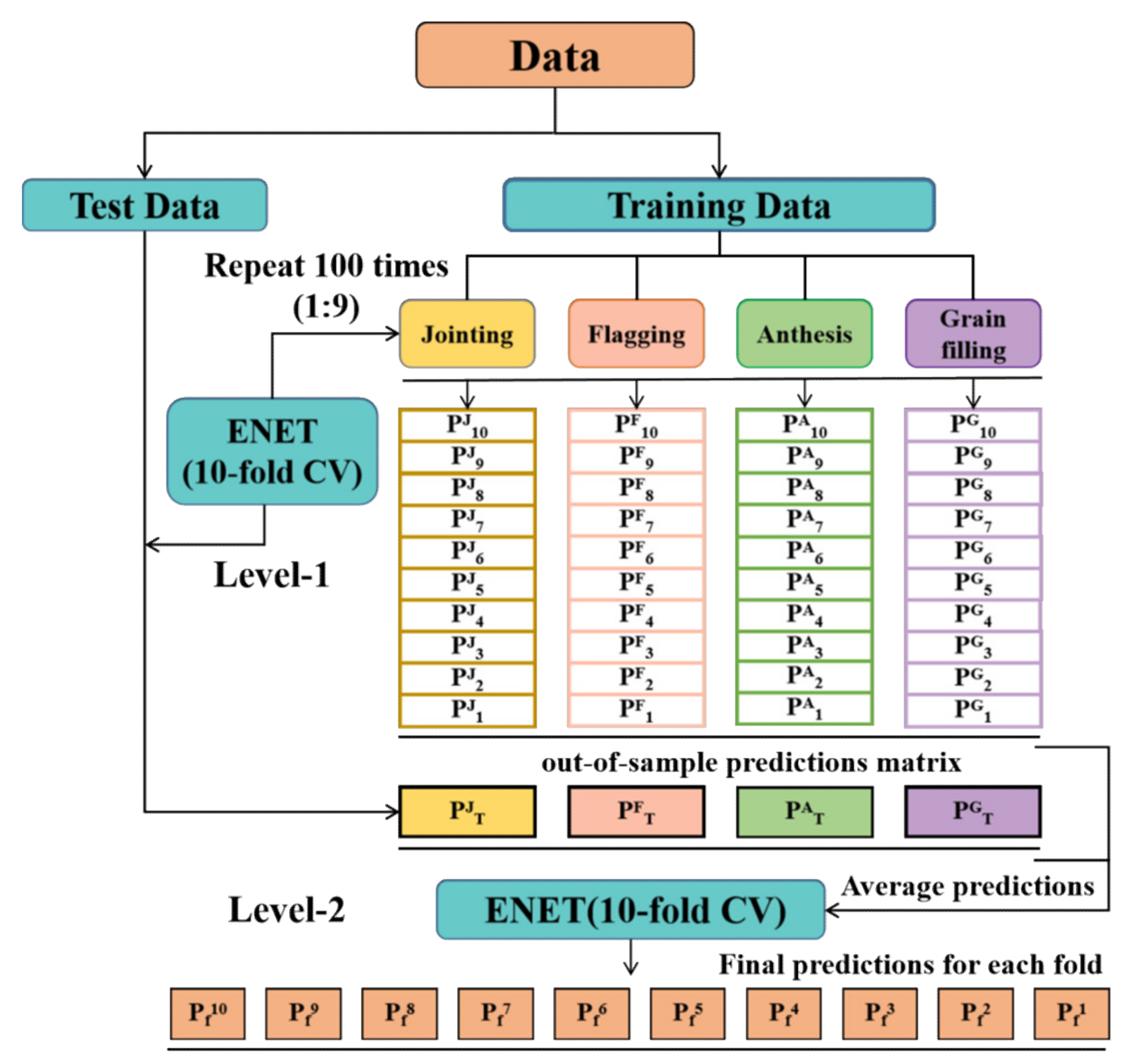
2.3.4. Stacking Technology

Ensemble learning can achieve better generalization performance than using a single learner by constructing and combining multiple learners. Based on the different strategies of the learner combination, it can be divided into boosting, bagging, and stacking learning methods [37]. Among them, stacking is a typical representative of the learning method, which learns how to best combine the predictions from multiple machine learning models with good performance and is typically used to generate a set of heterogeneous prediction variables. The basic idea of stacking regression is as follows: first, the entire training set is divided into T blocks by bootstrapped sampling, and the subset of T-1 blocks is randomly selected for model training of the primary learners. The model is tested on the remaining subset. Subsequently, through the training of the primary learner, the output of various learners is used as input of the next level to train the secondary learner to obtain a final output. Figure 3 showed the working principal diagram of this study based on the use of the stacking regression technology to predict the yield of winter wheat.

The stacking method of different growth periods is similar to the stacking method of the regression model, and the entire process is divided into two levels. In this study, the ENET was used as the primary model and the secondary model for testing, to effectively avoid collinearity between the yield prediction results of each growth period of the winter wheat because of the overlap of information. First, the dataset was randomly and evenly divided into 10 parts, 9 of which were randomly selected as the original training dataset to train the first-level learner, and the remaining one was used as the model test set. Subsequently, the primary model was trained with ten-fold cross-validation to obtain the prediction of each fold, and the results were collected in the prediction matrix outside the sample. At the same time, the 10 models trained in the test set were used to predict the yield of winter wheat. The results produced 10 groups of predicted values in the test set, and the average predicted value was calculated. In this study, the regression models of the four growth stages were tested, and the outputs of each primary model were used as input to the secondary model to train again, thus integrating the prediction ability of the multiple growth stages. Similarly, ten-fold cross-validation was also used in the secondary model to obtain the final predicted value to minimize model uncertainty. To compare the prediction accuracies of the different models more fairly, the dataset was divided into training set and test set with a sampling strategy of 9:1, which was repeated 100 times, and the same ten-fold cross-validation was performed on the primary model and the secondary model in each division process. Finally, 1000 models were generated, and the average values of the coefficient of determination (R²) and root-mean-square error (RMSE) on these 1000 test sets were used as the final evaluation index of the model. The stacking regression framework was built in R v4.0.2.

2.3.5. Cross-Validation

Cross-validation [65,66], also known as rotation estimation, this theory was proposed by Seymour [67]. It is a statistically practical method of cutting data samples into smaller subsets. Typically, it is used as an accuracy test and hyperparameter screening method when the amount of sample data is small. This study used 10-fold cross-validation to determine the best parameters of the model to obtain a model with higher accuracy. By dividing the dataset into 10 parts, 9 of them were used as training data in turn, and the remaining one was used as test data. Each test yielded a corresponding accuracy. The average error rate of 10 results was used to estimate the accuracy of the algorithm. The advantage of this method is that the randomly generated sub samples could be repeatedly used for training and verification, and the results could be verified each time.

2.3.6. Model Performance Evaluation

The coefficient of determination (R²) and the root-mean-square error (RMSE) were selected as the evaluation indicators of the modeling accuracy and verification accuracy. The closer the R² value to 1 and the lower the RMSE value, the better the model fitting effect. The calculation method is as follows:

$${\mathrm{R}}^2=\frac{({\displaystyle {\sum }_{i=1}^n{y}_i-\overline{y}{)}^2}}{({\displaystyle {\sum }_{i=1}^n{x}_i-\overline{y}{)}^2}},$$

(3)

$$\mathrm{RMSE}=\sqrt{\frac{{\displaystyle {\sum }_{i=1,j=1}^n{(x_i-y_i)}^2}}{n}},$$

(4)

where $x_i$ is the measured value of the yield; $y_i$ is the predicted value of yield; $\overline{y}$ is the average yield; n is the number of samples.

2.3.7. t-test

The t-test [68], also known as the student’s test, uses the t-distribution theory to infer the probability of the differences. Typically, in the case of small sample data, the t-test is performed to determine whether the p value is greater than 0.05 to compare whether the difference between the two sets of data is significant. If p < 0.05, there is a significant difference between the two groups. If p > 0.05, there is little possibility of a significant difference between the two groups. The calculation formula is as follows:

$$t=\frac{{{\displaystyle \overline{X}}}_1-{{\displaystyle \overline{X}}}_2}{\sqrt{\frac{({{\displaystyle n}}_1-1){{\displaystyle S}}_1^2 + ({{\displaystyle n}}_2-1){{\displaystyle S}}_2^2}{{{\displaystyle n}}_1 + {{\displaystyle n}}_2-2}(\frac{1}{{{\displaystyle n}}_1} + \frac{1}{{{\displaystyle n}}_2})}},$$

(5)

where ${\overline{X}}_1$ and ${\overline{X}}_2$ are the mean values of two samples; ${{\displaystyle S}}_1^2$ and ${{\displaystyle S}}_2^2$ are their variances; $n_1$ and $n_2$ are the two sample sizes, respectively.

3. Results

3.1. Phenotypic Analysis

The measured GY of each plot was obtained in the winter wheat harvest period, and the main statistical parameters of GY from different growing seasons were shown in

Table 2. Main statistical parameters of grain yield from different growing seasons.

Measurement Dates	MEAN (t ha−1)	SD (t ha−1)	CV (%)
2016–2017	5.84	0.95	16.27
2017–2018	6.35	1.12	17.64
2016–2018	6.10	1.24	20.33

SD means standard deviation; CV means coefficient of variation.

. The results show that the coefficient of variation (CV) values of GY from both growing seasons separately were similar, while the CV of overall GY from both growing seasons had elevated compared to the results from single growing season only.

LAI measured values of each plot were obtained the jointing, flagging, anthesis, and grain filling stages of winter wheat, and the main statistical parameters and variation characteristics of LAI were shown in

Table 3. Main statistical parameters of LAI from each growth stage in different growing seasons.

Measurement Dates	2016–2017			2017–2018			2016–2018
	MEAN	SD	CV (%)	MEAN	SD	CV (%)	MEAN	SD	CV (%)
Jointing	2.71	0.52	19.19	3.23	0.59	18.27	2.97	0.66	22.20
Flagging	3.26	0.61	18.71	3.93	0.61	15.52	3.60	0.69	19.17
Anthesis	3.45	0.68	19.71	4.3	0.81	18.84	3.88	0.87	22.42
Grain filling	1.85	0.71	38.38	1.97	0.74	37.56	1.91	0.76	39.79

SD means standard deviation; CV means coefficient of variation.

. Overall, the mean values of LAI from different growing seasons all showed a trend of increasing and then decreasing with the advancement of the fertility period, with the greatest increase rate of LAI from the jointing stage to the flagging stage and the peak of LAI at the anthesis stage, and the smallest mean value of LAI at the grain filling stage. In addition, the CV of LAI from single growing seasons were similar, while the CV of LAI from both growing seasons were significantly higher.

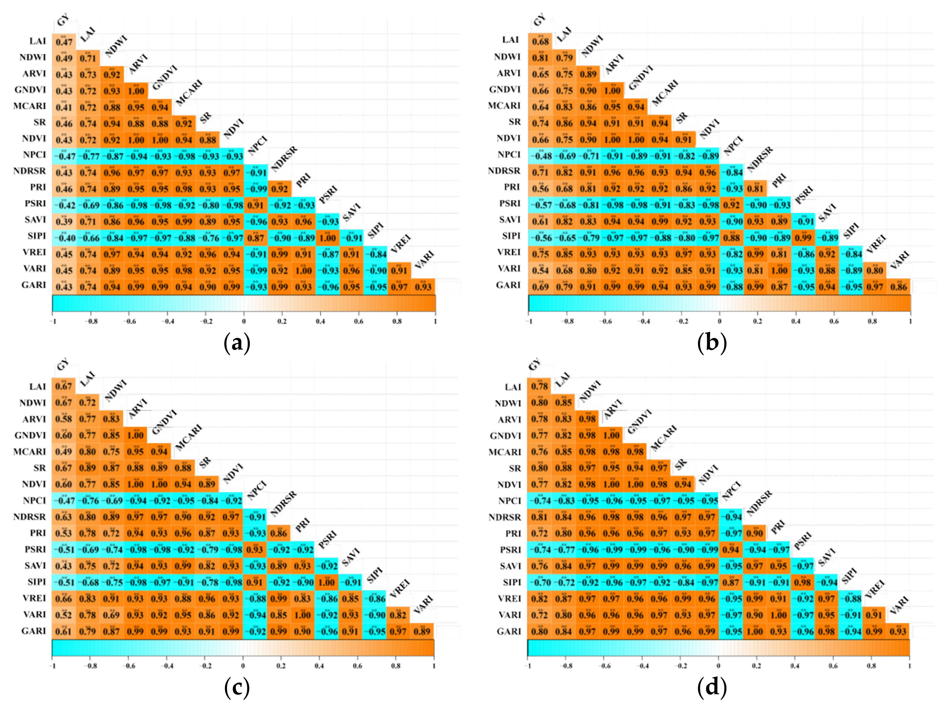
3.2. Correlations between Hyperspectral Vegetation Indices and Grain Yield

A correlation analysis between GY and 15 hyperspectral vegetation indices and LAI at the jointing, flagging, anthesis, and grain filling stages of wheat was conducted, as shown in Figure 4. The results showed that at the jointing stage, the absolute value of the correlation coefficient (|r|) between GY and 15 vegetation indices and LAI ranged from 0.39 to 0.49, and the absolute value of the correlation coefficient between NDWI and GY was the highest, with the best correlation (|r| = 0.49). At the flagging stage, the |r| value between GY and indices ranged from 0.47 to 0.67, among which the absolute value of the NDWI and GY correlation coefficient was the highest, that was, the strongest correlation (|r| = 0.67). At the anthesis stage, the |r| value between GY and the indices ranged from 0.48 to 0.81, and the absolute value of the correlation coefficient between NDWI and GY was the highest (|r| = 0.81). In the grain filling period, the |r| value between GY and the indices was between 0.7 and 0.82, and the correlation between the VREI and GY was the strongest (|r| = 0.82). The results showed that the correlation coefficients of LAI and GY were 0.47, 0.67, 0.68, and 0.78 at the jointing, flagging, anthesis, and grain filling stages, respectively. Overall, the correlation between GY and the hyperspectral vegetation indices and LAI showed the gradually increasing trend as the growth period progressed. All indices of each growth period were significantly correlated with GY (p < 0.001), which could be used to predict the yield of winter wheat. The correlations between different indices were shown in the attached Figure A2.

3.3. Elastic Network for Grain Yield Prediction

Based on the ENET, the vegetation indices and the vegetation indices coupled LAI were used as the input factors for the model to construct GY prediction models for four growth stages, respectively. Based on the prediction results, the box-plot of GY prediction accuracy for each growth stage was drawn with or without LAI, as shown in Figure 5.

Only 15 vegetation indices were used as the input features of the model to construct the GY prediction model for each growth period. The results showed that GY prediction accuracy at the jointing stage was R² = 0.20, RMSE = 1.33 t ha⁻¹; the GY prediction accuracy at the flagging stage was R² = 0.40, RMSE = 1.18 t ha⁻¹; the GY prediction accuracy at the anthesis stage was R² = 0.56, RMSE = 1.06 t ha⁻¹; the GY prediction accuracy during the grain filling period was R² = 0.60, RMSE = 0.94 t ha⁻¹. The above results show that the prediction accuracy R² of the GY prediction model based on the vegetation indices increased with the growth period and that the RMSE decreased with the growth of winter wheat, indicating that GY prediction ability for winter wheat increased with the growth period and reached the best prediction effect at the grain filling stage.

To study the influence of LAI on the accuracy of winter wheat GY prediction model, 15 vegetation indices of the four growth periods coupled with LAI of the same growth period were used as input factors for the model to construct a single-growth-period GY prediction model. The results showed that R² = 0.22, RMSE = 1.31 t ha⁻¹ at the jointing stage, R² = 0.49, RMSE = 1.1 t ha⁻¹ at the flagging stage, R² = 0.58, RMSE = 1.02 t ha⁻¹ at the anthesis stage, and R² = 0.66, RMSE = 0.88 t ha⁻¹ at the grain filling stage. Overall, the prediction accuracy of GY of winter wheat gradually increased with the growth period, and the prediction accuracy of the model at the grain filling stage was the highest.

The results showed that the 15 vegetation indices could be coupled with LAI to construct a GY prediction model. During the jointing, flagging, anthesis, and grain filling stages, the average R² of GY prediction model increased by 10%, 22.5%, 3.6% and 10%, the average RMSE were reduced by 1.5%, 6.7%, 3.8%, and 6.4%, respectively. A comparative analysis of the above results showed that GY prediction accuracy of each growth period had been improved after coupling the vegetation indices with LAI. Among them, the GY prediction accuracy of the flagging stage had improved the most.

To further verify the performance of GY prediction by coupling LAI with the vegetation indices, a paired t-test was used to evaluate whether there was a significant difference in the impact of vegetation indices on GY prediction accuracy when coupling with LAI, as listed in

Table 4. Results from the paired sample t-test.

Growth Stage	t	p Value
Jointing	12.135	0.000
Flagging	32.264	0.000
Anthesis	9.106	0.000
Grain filling	26.525	0.000

.

The results showed that the p-values for all four growth stages were less than 0.05, indicating that the vegetation indices coupled with LAI were used to construct GY prediction models with statistically significant improvement in prediction accuracy. The T value of the flagging stage was the highest (t = 32.264), and the accuracy was improved most evidently.

As shown in Figure A3, the Pearson’s correlations between the GY predictions for the four individual growth stages were high (r = 0.6–0.95). By contrast, the density curves of the grain yield predictions were slightly different from each other. Moreover, the base learners differed significantly in the distribution interval of the prediction accuracy.

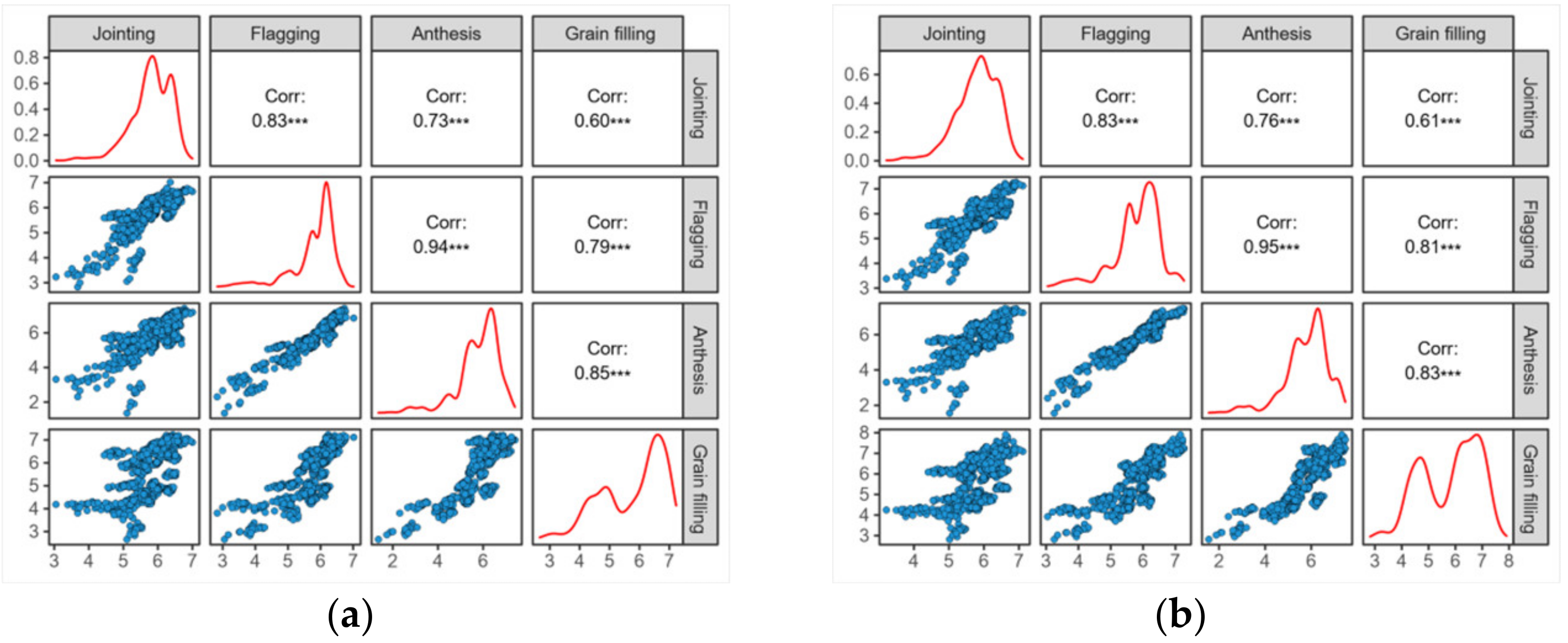
3.4. Comparative Analysis of Grain Yield Prediction Accuracy from Multiple Growth Stages

To evaluate the performance of the stacking method, the ENET algorithm was used as a secondary model to construct GY prediction model by integrating the prediction results of the four growth stages with and without coupled LAI in two cases, respectively. The accuracy of GY prediction results obtained by combining four of the base learners were presented in Figure 6.

The GY prediction model based on multiple growth stages was constructed using only the vegetation indices as the input factors for the model. The average prediction accuracy of the integrated model was R² = 0.67, RMSE = 0.85 t ha⁻¹. Overall, the GY prediction accuracy of the integrated multiple growth stages had been improved to varying degrees compared with the four single growth stages. Compared with the prediction accuracy of GY at the jointing, flagging, anthesis, and grain filling stages, the average R² of the integrated model increased by 235%, 67.5%, 19.6% and 11.7%, and the average RMSE decreased by 36.1%, 28%, 19.8%, and 9.6%, respectively.

The vegetation indices coupled with LAI were used as the input factors of the model to construct a GY prediction model by integrating multiple growth stages. The results showed that the prediction accuracy of the integrated model was R² = 0.74, RMSE = 0.81 t ha⁻¹. Overall, after integrating the multiple growth stages, the prediction accuracy of GY had been improved to varying degrees. Compared with the jointing, flagging, anthesis and grain filling stages, the average R² values of the integrated model increased by 236%, 51%, 27.6% and 12.1%, and the average RMSE decreased by 38.2%, 26.4%, 20.6%, and 8%, respectively. Based on the analysis of the above research results, the vegetation indices coupled with LAI were used as the model input factors, and based on the stacking technology, a GY prediction model integrating the four growth stages was constructed, yielding highest verification accuracy (R² = 0.74, RMSE = 0.81 t ha⁻¹).

To further verify whether the improvement in GY prediction accuracy by integrating information from multiple growth stages is significant, paired samples t-tests were used to assess whether there is a statistical difference in the validation R² between the integrated model and the single-growth stage model under two cases of vegetation indices with and without coupled LAI, respectively. The results were listed in

Table 5. Results from the paired sample t-test.

	Model	t	p Value
Without LAI	Ensemble vs. Jointing	51.153	0.000
	Ensemble vs. Flagging	39.902	0.000
	Ensemble vs. Anthesis	17.029	0.000
	Ensemble vs. Grain filling	15.711	0.000
With LAI	Ensemble vs. Jointing	60.18	0.000
	Ensemble vs. Flagging	39.092	0.000
	Ensemble vs. Anthesis	23.188	0.000
	Ensemble vs. Grain filling	16.646	0.000

.

The results showed that the integrated model outperformed the other base models with or without LAI, and the p values were less than 0.05 indicating that the accuracy improvement obtained by the integrated model was statistically significant. This further demonstrated the effectiveness of the stacking technique proposed in this paper for GY prediction. Among them, the accuracy of the jointing stage was improved most evidently, and the t value was the highest (t = 51.153 and t = 60.18, respectively), consistent with the above results. Moreover, when the vegetation indices coupled with LAI were used as the input factors of the model, the prediction accuracy of the integrated model improved more evidently, and GY prediction effect was better.

3.5. Weight Results for the Secondary Models

To determine the weight of each growth stage in the model stacking process, the regression coefficients of the prediction results of each growth period in the secondary model were statistically analyzed with and without coupling LAI, as shown in Figure 7.

The results showed that when only the vegetation indices were used as the input factors for GY prediction model, the average regression coefficients of the jointing, flagging, anthesis, and grain filling stages in the integrated model were 0.04, 0.05, 0.49, and 0.66, respectively. In the case of vegetation indices coupled with LAI, a GY prediction model integrating multiple growth stages was constructed, and the average regression coefficients of the jointing, flagging, anthesis, and grain filling stages were 0.06, 0.23, 0.48, and 0.72, respectively. Overall, with the development of the growth period, the proportion of each growth stage in the integrated model showed a gradual upward trend, in which the average regression coefficient of the grain filling stage and the weight were the highest. Compared with only using vegetation indices for GY prediction, after coupling the vegetation indices with LAI, the weight of the jointing, flagging, and grain filling stages in the integrated model all increased, while the weight of the anthesis stage decreased slightly, and the weight of the flagging stage increased most evidently.

4. Discussion

This study aims to improve the accuracy and robustness of crop yield prediction models. In this study, the data of two planting seasons from 2016 to 2018 were used to evaluate the improvement effect of GY prediction model. The information from multiple cropping seasons increased the variability of the data (Table 2 and Table 3), which was due to the differences in environmental and phenological conditions between different years and enhanced the prediction accuracy and transferability of the model. In recent years, hyperspectral remote sensing has great potential for application in rapid and accurate estimation of crop parameters and yields in agricultural fields because of its advantages of narrow waveband and strong continuity [69]. Considering the information overlap between adjacent bands, 15 vegetation indices were calculated in this study for constructing the GY prediction model instead of all bands in order to avoid generating data redundancy. These indices are located in the visible red and near-infrared wavelengths, which are important for photosynthesis in plants and are often used for timely monitoring of vegetation cover and growth vigor, etc. [70]. The results of the correlation analysis (Figure 4) indicated that all vegetation indices performed a highly significant correlation with GY (p < 0.001). However, there are differences in the potential of different vegetation indices for GY prediction due to the fact that the vegetation information obtained from different spectral channels has various correlations with different elements of vegetation or a certain character state. The NDWI index showed a high correlation with GY due to its ability to effectively extract the water content of the vegetation canopy and respond to moisture changes in a timely manner [71]. The VREI index provides a timely response to changes in chlorophyll concentration, canopy structure and water content in plants, and is often used in vegetation phenology change monitoring, precision agriculture and vegetation productivity modeling [59]. The vegetation cover will change as the fertility period advances, and the effect of soil background can be effectively reduced by introducing MCARI and SAVI. The ARVI can effectively reduce the dependence of spectral reflectance on atmospheric properties [48], which is important for the transfer of models to airborne remote sensing platforms. NDVI eliminates most of the variation in irradiance associated with instrument calibration, sun angle, topography, cloud shadows, and atmospheric conditions, enhancing the response to vegetation [52]. PRI is sensitive to changes in carotenoid content in plants and gradually increases in correlation with GY during late crop growth. SIPI and PSRI indices are often used for canopy physiological stress monitoring and crop yield analysis [56,58]. In addition, the correlation between the same vegetation index and GY varies at different growth stages. This is due to the fact that as the crop fertility progresses, the growth and development of the plant and the influence of the external environment led to changes in its internal components and structure, which cause the spectral characteristics of the plant canopy or leaves to change subsequently [72]. Thus, the combination of multiple vegetation indices used to construct the GY prediction model can achieve complementary information to overcome the limitations of a single band or a single index, which effectively improves the prediction accuracy and robustness of the model (

Table A7. Statistical analysis of GY prediction accuracy for a single optimal variable and multiple variables.

Growth Stage	Input Features	R2	RMSE (t ha−1)
Jointing	NDWI	0.16	1.38
	VIs	0.2	1.33
Flagging	NDWI	0.18	1.36
	VIs	0.4	1.18
Anthesis	NDWI	0.42	1.2
	VIs	0.56	1.06
Grain filling	VREI	0.54	1.08
	VIs	0.6	0.94

VIs means 15 vegetation indices.

). This has important significance for the transfer of the model to practical applications.

The essence of yield formation is the complex process of production, transportation, accumulation, and distribution of photosynthetic products [73]. As the reproductive period advances, spectral saturation of the vegetation index occurs when the vegetation cover is greater than 80%. In this study, the coupling of structural parameters (LAI) and spectral parameters (vegetation indices) of the crop effectively improved the accuracy of GY prediction at each growth stage, and the results of the t-test (Table 4) also fully demonstrated that the improvement of model effects at each growth stage was significant (p < 0.05). This is because LAI is an important canopy structure information of crops and one of the important variables to determine the intensity of photosynthesis [4,74]. The size of vegetation leaf area directly affects light interception, photosynthesis and transpiration efficiency of vegetation canopy, and is considered to be the most important factor affecting plant productivity [75]. The results are consistent with those reported by Delécolle et al. [24] and Wang et al. [76]. Among them, the most significant improvement in model accuracy was observed in the flagging stage (the relative value of R² increased by 22.5%) which is consistent with our statistical t-test (t = 32.264). This is because the flagging stage is a critical period for the formation of wheat spike number, and this growth stage is mainly reflected in the rapid growth of leaf area and the consequent increase in photosynthetic efficiency, which contributes more to the accumulation of dry matter [77]. Our study demonstrated that canopy spectral saturation can be effectively overcome by coupling LAI and vegetation indices, and this study can provide a new method for accurate and rapid estimation of crop yield.

The results of GY estimation at single growth stage indicated that there were significant differences in yield estimation at different fertility stages, which showed an increasing accuracy of prediction with the advancement of growth stage. This is because crop growth and development is a dynamic and continuous process, and changes in the growth state and environmental characteristics of the crop at each growth stage can lead to different morphological characteristics of the spectral curve, and thus the accuracy of the yield estimation models at different growth stages varies. Since each key stage of crop growth and development can have a significant impact on yield formation, it is important to find a method to combine information from multiple growth stages to improve the accuracy and robustness of the model. The objective of employing a stacking technique was to improve the prediction ability by combining data from multiple growth stages instead of using single growth stage data. When implementing a stacking approach, it is necessary to include self-sufficient, independent, and diverse base learners for analysis (Figure A3) [47]. The results showed that there was a strong correlation between the predicted results of different growth stages (correlation coefficients of R = 0.6–0.95), which was due to the overlap of information between adjacent fertility stages. ENET is used as a secondary model to perform the multicollinearity data analysis in the model when stacking multiple base learners due to its advantages of both ridge regression and lasso regression [63]. In this study, vegetation indices and LAI from four key growth stages of the crop were successfully combined to achieve higher accuracy in predicting grain yield than any single growth stage (Figure 5 and Figure 6). In addition, the accuracy parameters (R² and RMSE) of the base learner fluctuated more and had a wider range than those of the ensemble approach, which also demonstrated the stability of the GY model constructed based on the Stacking technique. However, stacking techniques are sensitive to the timing of data collection at different growth stages. Due to the differences in developmental rates of different varieties, this may lead to the fact that different varieties may be at different growth stages at the same time. In addition, due to the different gradients of water and fertilizer stress treatments, which may have an impact on the growth and development rate of the crop, this poses a significant challenge to our data collection process.

The analysis of the regression coefficients combining the four base learners showed that the highest weight was given to the grain filling stage with or without LAI, which is consistent with the highest accuracy of the previous prediction of the grain filling stage. Therefore, the use of the grain filling stage as a key learner in the grain yield prediction has a very positive effect on the improvement of the prediction effectiveness of the ensemble model. This is rational since grain filling is the stage where wheat transfers organic matter such as starch and protein produced by photosynthesis from the vegetative organs to the grains, and the vegetation indexes in this period are closely related to the final quality of thousand-grain weight [29]. However, the regression coefficients for the jointing period showed negative values in some cases, which is obviously detrimental to improving the model accuracy. The reason for this phenomenon is that the crop cover is small and the ground surface is exposed at the jointing stage, so it is easy to be disturbed by the soil background and other factors during the spectral data collection [78]. Moreover, the LAI at this stage is relatively small and photosynthesis is weak, resulting in the accumulation of little dry matter yet, and its contribution in the integrated model is poor compared to other growth stages. The t-test results (Table 5) show that the GY prediction model with stacked four growth stages performed with good accuracy and robustness than any single growth stage, which has important implications for the practical application of the prediction model.

5. Conclusions

Winter wheat is one of the most widely grown grain crops in the world, and pre-harvest insights into yields can help optimize management practices. In this study, we developed an ensemble learning framework for stacking information from multiple growth stages of the crop. The results showed that the ensemble model outperformed other individual growth stage models. In addition, coupling vegetation indices with LAI can effectively overcome the spectral saturation phenomenon and improve the prediction accuracy of the model. Our study demonstrated the effectiveness of Stacking technique for improving GY prediction accuracy (Figure A4), which can provide new ideas for yield estimation of other crops.

References

1. Yang, M.; Adeel, H.M.; Xu, K.; Zheng, C.; Rasheed, A.; Zhang, Y.; Jin, X.; Xia, X.; Xiao, Y.; He, Z. Assessment of Water and Nitrogen Use Efficiencies Through UAV-Based Multispectral Phenotyping in Winter Wheat. Front. Plant Sci. 2020, 11, 927. [Google Scholar] [CrossRef]
2. Hutchinson, C.F. Uses of satellite data for famine early warning in sub-Saharan Africa. Int. J. Remote Sens. 1991, 12, 1405–1421. [Google Scholar] [CrossRef]
3. Franch, B.; Vermote, E.F.; Becker-Reshef, I.; Claverie, M.; Huang, J.; Zhang, J.; Justice, C.; Sobrino, J. Improving the timeliness of winter wheat production forecast in the United States of America, Ukraine and China using MODIS data and NCAR Growing Degree Day Information. Remote Sens. Environ. 2015, 161, 131–148. [Google Scholar] [CrossRef]
4. Chen, Y.; Zhang, Z.; Tao, F. Improving regional winter wheat yield estimation through assimilation of phenology and leaf area index from remote sensing data. Eur. J. Agron. 2018, 101, 163–173. [Google Scholar] [CrossRef]
5. Vanli, Ö.; Ahmad, I.; Ustundag, B.B. Area estimation and yield forecasting of wheat in southeastern turkey using a machine learning approach. J. Indian Soc. Remote Sens. 2020, 48, 1757–1766. [Google Scholar] [CrossRef]
6. Wu, S.; Yang, P.; Ren, J.; Chen, Z.; Li, H. Regional winter wheat yield estimation based on the wofost model and a novel vw-4densrf assimilation algorithm. Remote Sens. Environ. 2021, 255, 112276. [Google Scholar] [CrossRef]
7. Hatfield, J.L.; Prueger, J.H. Value of using different vegetative indices to quantify agricultural crop characteristics at different growth stages under varying management practices. Remote Sens. 2010, 2, 562–578. [Google Scholar] [CrossRef] [Green Version]
8. Tao, H.; Feng, H.; Xu, L.; Miao, M.; Yang, G.; Yang, X.; Fan, L. Estimation of the yield and plant height of winter wheat using UAV-based hyperspectral images. Sensors 2020, 20, 1231. [Google Scholar] [CrossRef] [Green Version]
9. Cao, J.; Zhang, Z.; Luo, Y.; Zhang, L.; Zhang, J.; Li, Z. Wheat yield predictions at a county and field scale with deep learning, machine learning, and google earth engine. Eur. J. Agron. 2021, 123, 126204. [Google Scholar] [CrossRef]
10. Liu, C.; Chen, Z.; Shao, Y.; Chen, J.; Tuya, H.; Pan, H. Research advances of sar remote sensing for agriculture applications: A review. J. Integr. Agric. 2019, 18, 506–525. [Google Scholar] [CrossRef] [Green Version]
11. Wang, P.; Li, Z.; Li, J.; Schmit, T.J. Added-value of geo-hyperspectral infrared radiances for local severe storm forecasts using the hybrid osse method. Ad. Atmos. Sci. 2021, 38, 1315–1333. [Google Scholar] [CrossRef]
12. Fletcher, R.S. Using vegetation indices as input into random forest for soybean and weed classification. Am. J. Plant. Sci. 2016, 7, 2186–2198. [Google Scholar] [CrossRef] [Green Version]
13. Wang, K.; Wang, X. Research on winter wheat yield estimation with the multiply remote sensing vegetation index combination. J. Arid Land Resour. Environ. 2017, 31, 44–49. [Google Scholar]
14. Tao, H.; Xu, L. Winter wheat yield estimation based on UAV hyperspectral remote sensing data. Trans. Chin. Soc. Agric. Mach. 2020, 51, 146–155. [Google Scholar]
15. Montesinos-López, O.A.; Montesinos-López, A.; Crossa, J.; de los Campos, G.; Alvarado, G.; Suchismita, M.; Jessica Rutkoski, J.; González-Pérez, L.; Burgueño, J. Predicting grain yield using canopy hyperspectral reflectance in wheat breeding data. Plant Methods 2017, 13, 4. [Google Scholar] [CrossRef] [Green Version]
16. Parker, J.E.; Crowder, D.W.; Eigenbrode, S.D. Trap crop diversity enhances crop yield. Agric. Ecosys. Environ. 2016, 232, 254–262. [Google Scholar] [CrossRef] [Green Version]
17. Sadeghi-Tehran, P.; Virlet, N.; Ampe, E.M.; Reyns, P.; Hawkesford, M.J. Deepcount: In-field automatic quantification of wheat spikes using simple linear iterative clustering and deep convolutional neural networks. Front. Plant Sci. 2019, 10, 1176. [Google Scholar] [CrossRef] [PubMed]
18. Yao, X.; Wang, N.; Liu, Y.; Cheng, T.; Tian, Y.; Chen, Q.; Zhu, Y. Estimation of Wheat LAI at Middle to High Levels Using Unmanned Aerial Vehicle Narrowband Multispectral Imagery. Remote Sens. 2017, 9, 1304. [Google Scholar] [CrossRef] [Green Version]
19. Shi, X.; Yu, Z.; Zhao, J.; Shi, Y.; Wang, X. Effect of Nitrogen Application Rateon Photosynthetic Characteristics, Dry Matter Accumulation and Distribution and Yield of High-Yielding Winter Wheat. J. Triticeae Crops 2021, 41, 713–721. [Google Scholar]
20. Novelli, F.; Spiegel, H.; Sandén, T.; Vuolo, F. Assimilation of sentinel-2 leaf area index data into a physically-based crop growth model for yield estimation. Agronomy 2019, 9, 255. [Google Scholar] [CrossRef] [Green Version]
21. Song, Y.; Wang, J.; Shang, J.; Liao, C. Using UAV-based SOPC derived LAI and SAFY model for biomass and yield estimation of winter wheat. Remote Sens. 2020, 12, 2378. [Google Scholar] [CrossRef]
22. Li, C.; Ma, C.; Cui, Y.; Lu, G.; Wei, F. Uav hyperspectral remote sensing estimation of soybean yield based on physiological and ecological parameter and meteorological factor in china. J. Indian Soc. Remote 2020, 49, 873–886. [Google Scholar] [CrossRef]
23. Dente, L.; Satalino, G.; Mattia, F.; Rinaldi, M. Assimilation of leaf area index derived from asar and meris data into ceres-wheat model to map wheat yield. Remote Sens. Environ. 2007, 112, 1395–1407. [Google Scholar] [CrossRef]
24. Delécolle, R.; Maas, S.J.; Guérif, M.; Baret, F. Remote sensing and crop production models: Present trends. ISPRS J. Photogramm. 1992, 47, 145–161. [Google Scholar] [CrossRef]
25. Hasan, M.M.; Chopin, J.P.; Laga, H.; Miklavcic, S.J. Detection and analysis of wheat spikes using convolutional neural networks. Plant Methods 2018, 14, 100. [Google Scholar] [CrossRef] [Green Version]
26. Wu, X.; Tang, Y.; Li, C.; Wu, C.; Huang, G. Effect of waterlogging at different growth stages on flag leaf chlorophyll fluorescence and grain-filling properties of winter wheat. Chin. J. Eco-Agric. 2015, 23, 309–318. [Google Scholar]
27. Jin, P.; Ru, Z.; Zhou, M.; Hou, Y.; He, H.; Luo, Y. Effects of low temperature and overcast rainy during spring on the yield characters of wheat. Crops Res. 2010, 24, 103–108. [Google Scholar]
28. Chen, J.; Zhang, F.; Zhou, H.; Zhao, Y.; Wei, X. Effect of irrigation at different growth stages and nitrogen fertilizer on maize growth, yield and water use efficiency. J. Northwest A F Univ.-Nat. Sci. Ed. 2011, 39, 322–331. [Google Scholar]
29. Guan, K.; Wu, J.; Kimball, J.S.; Anderson, M.C.; Frolking, S.; Li, B.; Hain, C.R.; Lobell, D.B. The shared and unique values of optical, fluorescence, thermal and microwave satellite data for estimating large-scale crop yields. Remote Sens. Environ. 2017, 199, 333–349. [Google Scholar] [CrossRef] [Green Version]
30. Hernandez, J.; Lobos, G.; Matus, I.; del Pozo, A.; Silva, P.; Galleguillos, M. Using ridge regression models to estimate grain yield from field spectral data in bread wheat (Triticum aestivum L.) grown under three water regimes. Remote Sens. 2015, 7, 2109–2126. [Google Scholar] [CrossRef] [Green Version]
31. Tan, H.; Li, S.; Wang, K.; Xie, R.; Gao, S.; Ming, B.; Qing, Y.; Lai, J.; Liu, G.; Tang, Q. Monitoring canopy chlorophyll density in seedlings of winter wheat using imaging spectrometer. Acta Agron. Sin. 2008, 34, 1812–1817. [Google Scholar] [CrossRef]
32. Sun, B.Y.; Chang, Q.R.; Liu, M.Y. Inversion chlorophyll mass fraction in winter wheat canopy by hyperspectral reflectance. Acta Agric. Boreali. Sin. 2017, 26, 552–559. [Google Scholar]
33. Patel, N.R.; Mohammed, A.J.; Rakhesh, D. Modeling of wheat yields using multi-temporal terra/modis satellite data. Geocarto Int. 2006, 21, 43–50. [Google Scholar] [CrossRef]
34. Li, R.; Li, C.; Xu, X.; Wang, J.; Yang, X.; Huang, W.; Pan, Y. Winter wheat yield estimation based on support vector machine regression and multi-temporal remote sensing data. Trans. Chin. Soc. Agric. Eng. 2009, 25, 114–117. [Google Scholar]
35. Li, Z.; Song, M.; Feng, H. Dynamic characteristics of leaf area index and plant height of winter wheat influenced by irrigation and nitrogen coupling and their relationships with yield. Trans. Chin. Soc. Agric. Eng. 2017, 33, 195–202. [Google Scholar]
36. Ghizlane, A.; Eddine, D.J.; Imane, S.; Samir, B.; Ettarid, M. Mapping wheat dry matter and nitrogen content dynamics and estimation of wheat yield using UAV multispectral imagery machine learning and a variety-based approach: Case study of morocco. AgriEngineering 2021, 3, 29–49. [Google Scholar]
37. Feng, L.; Zhang, Z.; Ma, Y.; Du, Q.; Williams, P.; Drewry, J.; Luck, B. Alfalfa yield prediction using UAV-based hyperspectral imagery and ensemble learning. Remote Sens. 2020, 12, 2028. [Google Scholar] [CrossRef]
38. Clinton, N.; Yu, L.; Gong, P. Geographic stacking: Decision fusion to increase global land cover map accuracy. ISPRS J. Photogramm. Remote Sens. 2015, 103, 57–65. [Google Scholar] [CrossRef]
39. Healey, S.P.; Cohen, W.B.; Yang, Z.; Brewer, C.K.; Brooks, E.B.; Gorelick, N.; Hernandez, A.; Huang, C.; Hughes, M.J.; Kennedy, R. Mapping forest change using stacked generalization: An ensemble approach. Remote Sens. Environ. 2018, 204, 717–728. [Google Scholar] [CrossRef]
40. Fu, P.; Meacham-Hensold, K.; Guan, K.; Bernacchi, C.J. Hyperspectral leaf reflectance as proxy for photosynthetic capacities: An ensemble approach based on multiple machine learning algorithms. Front. Plant Sci. 2019, 10, 730. [Google Scholar] [CrossRef] [PubMed]
41. Zhou, Z.; Yufang, J.; Bin, C.; Patrick, B. California almond yield prediction at the orchard level with a machine learning approach. Front. Plant Sci. 2019, 10, 809. [Google Scholar]
42. Durbin, R.; Willshaw, D. An analogue approach to the travelling salesman problem using an elastic net method. Nature 1987, 326, 689–691. [Google Scholar] [CrossRef] [PubMed]
43. Wang, Y.; Wang, S.; Zheng, Y.; Song, F.; Ma, Y.; Zhang, H. Calculation and allocation of operation and maintenance cost of power grid project based on elastic net. Autom. Electr. Power Syst. 2020, 44, 165–172. [Google Scholar]
44. Chen, Y.; Xiao, G.; Hu, M.; Huang, J. Dam deformation prediction based on extreme learning machine and elastic network. Sci. Surv. Mapp. 2020, 45, 20–27+40. [Google Scholar]
45. Osco, L.P.; Ramos, A.P.; Faita Pinheiro, M.M.; Moriya, É.A.S.; Imai, N.N.; Estrabis, N. A machine learning framework to predict nutrient content in valencia-orange leaf hyperspectral measurements. Remote Sens. 2020, 12, 906. [Google Scholar] [CrossRef] [Green Version]
46. Fei, S.; Hassan, M.A.; He, Z.; Chen, Z.; Shu, M.; Wang, J.; Li, C.; Xiao, Y. Assessment of ensemble learning to predict wheat grain yield based on UAV-multispectral reflectance. Remote Sens. 2021, 13, 2338. [Google Scholar] [CrossRef]
47. Gao, B.C. NDWI—A normalized difference water index for remote sensing of vegetation liquid water from space. Remote Sens. Environ. 1996, 58, 257–266. [Google Scholar] [CrossRef]
48. Miura, T.; Huete, A.R.; Yoshioka, H.; Holben, B.N. An error and sensitivity analysis of atmospheric resistant vegetation indices derived from dark target-based atmospheric correction. Remote Sens. Environ. 2001, 78, 284–298. [Google Scholar] [CrossRef]
49. Gitelson, A.A.; Merzlyak, M.N. Remote sensing of chlorophyll concentration in higher plant leaves. Adv. Space Res. 1998, 22, 689–692. [Google Scholar] [CrossRef]
50. Daughtry, C.S.T.; Walthall, C.L.; Kim, M.S.; De Colstoun, E.B.; McMurtrey, J.E., III. Estimating corn leaf chlorophyll concentration from leaf and canopy reflectance. Remote Sens. Environ. 2000, 74, 229–239. [Google Scholar] [CrossRef]
51. George, J.P.; Yang, W.; Kobayashi, H.; Biermann, T.; Carrara, A.; Cremonese, E.; Pisek, J. Method comparison of indirect assessments of understory leaf area index (LAlu): A case study across the extended network of ICOS forest ecosystem sites in Europe. Ecol. Indic. 2021, 128, 107841. [Google Scholar] [CrossRef]
52. Tucker, C.J. Red and photographic infrared linear combinations for monitoring vegetation. Remote Sens. Environ. 1979, 8, 127–150. [Google Scholar] [CrossRef] [Green Version]
53. Aparicio, N.; Villegas, D.; Royo, C.; Casadesus, J.; Araus, J.L. Effect of sensor view angle on the assessment of agronomic traits by ground level hyper-spectral reflectance measurements in durum wheat under contrasting mediterranean conditions. Int. J. Remote Sens. 2004, 25, 1131–1152. [Google Scholar] [CrossRef]
54. Gitelson, A.A.; Viña, A.; Ciganda, V.; Rundquist, D.C.; Arkebauer, T.J. Remote estimation of canopy chlorophyll content in crops. Geophys. Res. Lett. 2005, 32, L08403. [Google Scholar] [CrossRef] [Green Version]
55. Gamon, J.A.; Serrano, L.; Surfus, J.S. The photochemical reflectance index: An optical indicator of photosynthetic radiation use efficiency across species, functional types, and nutrient levels. Oecologia 1997, 112, 492–501. [Google Scholar] [CrossRef]
56. Ren, S.; Chen, X.; An, S. Assessing plant senescence reflectance index-retrieved vegetation phenology and its spatiotemporal response to climate change in the Inner Mongolian Grassland. Int. J. Biometeorol. 2017, 61, 601–612. [Google Scholar] [CrossRef] [PubMed]
57. Huete, A.; Didan, K.; Miura, T.; Rodriguez, E.P.; Gao, X.; Ferreira, L.G. Overview of the radiometric and biophysical performance of the modis vegetation indices. Remote Sens. Environ. 2002, 83, 195–213. [Google Scholar] [CrossRef]
58. Peñuelas, J.; Filella, I. Visible and near-infrared reflectance techniques for diagnosing plant physiological status. Trends Plant Sci. 1998, 3, 151–156. [Google Scholar] [CrossRef]
59. Manley, P.V.; Sagan, V.; Fritschi, F.B.; Burken, J.G. Remote sensing of explosives-induced stress in plants: Hyperspectral imaging analysis for remote detection of unexploded threats. Remote Sens. 2019, 11, 1827. [Google Scholar] [CrossRef] [Green Version]
60. Gitelson, A.A.; Kaufman, Y.J.; Stark, R.; Rundquist, D. Novel algorithms for remote estimation of vegetation fraction. Remote Sens. Environ. 2002, 80, 76–87. [Google Scholar] [CrossRef] [Green Version]
61. Monsef, H.A.E.; Smith, S.E. A new approach for estimating mangrove canopy cover using Landsat 8 imagery. Comput. Electron. Agric. 2017, 135, 183–194. [Google Scholar] [CrossRef]
62. Cao, Y.; Wu, Y.; Li, M.; Liang, W.; Zhang, P. PolSAR image classification using a superpixel-based composite kernel and elastic net. Remote Sens. 2021, 13, 380. [Google Scholar] [CrossRef]
63. Zou, H.; Hastie, T. Regularization and variable selection via the elastic net. J. R. Stat. Soc. Ser. B (Stat. Methodol.) 2005, 67, 301–320. [Google Scholar] [CrossRef] [Green Version]
64. Zheng, N.; Luan, X.; Liu, F. Near infrared spectroscopy modeling based on adaptive elastic net method. Spectrosc. Spect. Anal. 2018, 39, 319–324. [Google Scholar]
65. Dayananda, S.; Astor, T.; Wijesingha, J.; Chickadibburahalli Thimappa, S.; Dimba Chowdappa, H.; Mudalagiriyappa. Multi-temporal monsoon crop biomass estimation using hyperspectral imaging. Remote Sens. 2019, 11, 1771. [Google Scholar] [CrossRef] [Green Version]
66. Yang, Q.; Shi, L.; Han, J.; Zha, Y.; Zhu, P. Deep convolutional neural networks for rice grain yield estimation at the ripening stage using UAV-based remotely sensed images. Field Crops Res. 2019, 235, 142–153. [Google Scholar] [CrossRef]
67. Fisher, S. Boundary effects of persistent inputs and messages. J. Abnorm. Psychol. 1971, 77, 290–295. [Google Scholar] [CrossRef] [PubMed]
68. Napier-Munn, T.J.; Meyer, D.H. A modified paired t-test for the analysis of plant trials with data autocorrelated in time. Miner. Eng. 1999, 12, 1093–1100. [Google Scholar] [CrossRef]
69. Ma, Y.; Fang, S.; Peng, Y.; Gong, Y.; Wang, D. Remote estimation of biomass in winter oilseed rape (Brassica napus L.) using canopy hyperspectral data at different growth stages. Appl. Sci. 2019, 9, 545. [Google Scholar] [CrossRef] [Green Version]
70. Kong, L.A.; Wang, F.; Feng, B.; Li, S.; Si, J.; Zhang, B. A root-zone soil regime of wheat: Physiological and growth responses to furrow irrigation in raised bed planting in northern China. Agron. J. 2010, 102, 154–162. [Google Scholar] [CrossRef]
71. Bayat, B.; van der Tol, C.; Verhoef, W. Remote sensing of grass response to drought stress using spectroscopic techniques and canopy reflectance model inversion. Remote Sens. 2016, 8, 557. [Google Scholar] [CrossRef] [Green Version]
72. Liu, C.; Sun, P.; Liu, S. A review of plant spectral reflectance response to water physiological changes. Chin. J. Plant Ecol. 2016, 40, 80–91. [Google Scholar]
73. Zhang, J.; Zhang, H.; Li, S.; Li, J.; Yan, L.; Xia, L. Increasing yield potential through manipulating of an are1 ortholog related to nitrogen use efficiency in wheat by crispr/cas9. J. Integr. Plant Biol. 2021, 63, 1649–1663. [Google Scholar] [CrossRef]
74. Slamet, W.; Purbajanti, E.D.; Darmawati, A.; Fuskhah, E. Leaf area index, chlorophyll, photosynthesis rate of lettuce (Lactuca sativa L) under N-organic fertilizer. Indian J. Agric. Res. 2017, 51, 365–369. [Google Scholar] [CrossRef] [Green Version]
75. Ke, L.; Zhou, Q.; Wu, W.; Xia, T.; Tang, H. Estimating the crop leaf area index using hyperspectral remote sensing. J. Integr. Agric. 2016, 15, 475–491. [Google Scholar]
76. Wang, P.; Chen, C.; Zhang, S.; Zhang, Y.; Li, H. Winter wheat yield estimation based on copula function and remotely sensed LAI and VTCI. Trans. Chin. Soc. Agric. Mach. 2021, 52, 255–263. [Google Scholar]
77. Ren, J.; Chen, Z.; Zhou, Q.; Tang, H. Regional yield estimation for winter wheat with MODIS-NDVI data in Shandong, China. Int. J. Appl. Earth Obs. 2008, 10, 403–413. [Google Scholar] [CrossRef]
78. Zhang, Z.; Zhou, Y.; Yang, S.; Tan, C.; Lao, C.; Xu, C. Inversion Method for Soil Water Content in Winter Wheat Root Zone with Eliminating Effect of Soil Background. Trans. Chin. Soc. Agric. Mach. 2021, 52, 197–207. [Google Scholar]
Figure 1. Geographical location of study area.
Applsci 11 12164 g001
Figure 2. Technology roadmap.
Applsci 11 12164 g002
Figure 3. The workflow of the stacking regression model for predicting grain yield. In the figure: CV, cross-validation; P, prediction values of grain yield; J, jointing; F, flagging; A, anthesis; G, grain filling.
Applsci 11 12164 g003
Figure 4. Correlation between grain yield and indices of each growth stage.
Applsci 11 12164 g004
Figure 5. The statistical distributions of the prediction accuracy of each growth stage for grain yield prediction in the test phases; (a) distributions of R2 at each individual stage; (b) distributions of RMSE at the each individual stage.
Applsci 11 12164 g005
Figure 6. The statistical distributions of prediction accuracy of the stacking regression when including four growth stages for predicting grain yield in the test phases; (a) distributions of R2 without or with LAI coupling; (b) distributions of RMSE without or with LAI coupling.
Applsci 11 12164 g006
Figure 7. The distribution of regression coefficients for each growth stage within the level-2 model (ENET). (a) Without LAI; (b) With LAI.
Applsci 11 12164 g007