Article

Remote and Proximal Sensing Techniques for Site-Specific Irrigation Management in the Olive Orchard

1
Department of Agriculture, Food and Environment, University of Pisa, Via del Borghetto, 80, 56124 Pisa, Italy
2
Department of Agriculture and Forest Sciences, University of Tuscia, Via S.C. de Lellis, 01100 Viterbo, Italy
*
Author to whom correspondence should be addressed.
Appl. Sci. 2022, 12(3), 1309; https://doi.org/10.3390/app12031309
Submission received: 7 December 2021 / Revised: 13 January 2022 / Accepted: 24 January 2022 / Published: 26 January 2022

Abstract

:
The aim of this study was to evaluate the potential use of remote and proximal sensing techniques to identify homogeneous zones in a high density irrigated olive (Olea europaea L.) orchard subjected to three irrigation regimes (full irrigation, deficit irrigation and rainfed conditions). An unmanned aerial vehicle equipped with a multispectral camera was used to measure the canopy NDVI and two different proximal soil sensors to map soil spatial variability at high resolution. We identified two clusters of trees showing differences in fruit yield (17.259 and 14.003 kg per tree in Cluster 1 and 2, respectively) and annual TCSA increment (0.26 and 0.24 dm2, respectively). The higher tree productivity measured in Cluster 1 also resulted in a higher water use efficiency for fruit (WUEf of 0.90 g dry weight L−1 H2O) and oil (WUEo of 0.32 g oil L−1 H2O) compared to Cluster 2 (0.67 and 0.27 for WUEf and WUEo, respectively). Remote and proximal sensing technologies allowed to determine that: (i) the effect of different irrigation regimes on tree performance and WUE depended on the location within the orchard; (ii) tree vigour played a major role in determining the final fruit yield under optimal soil water availability, whereas soil features prevailed under rainfed conditions.

1. Introduction

Water availability is the main limiting factor for the growth and yield of crops in the Mediterranean region, which is expected to undergo dramatic changes in temperature and precipitation due to climate change [1,2]. Climate change will also likely increase the frequency of heat waves and prolonged periods of drought [3,4], inducing uncertainties about the potential productivity of crops. Irrigation can help to mitigate the impact of climate change on perennial crops, including olive trees. Although olive trees are drought tolerant, many studies showed the beneficial effects of irrigation on vegetative growth, yield components, and oil quality [5,6,7,8,9,10].
An important aspect in irrigation management is to understand the multiple interactions between water availability and soil properties or canopy vigour, which may potentially cause variations in yield and vegetative growth. In this respect, site-specific management of inputs, such as fertilizers and irrigation water, requires the understanding of the spatial distribution of soil characteristics, tree vigour, and productivity. Homogenous zones within the orchard for tree vigour and soil properties can be identified by soil sampling protocols and by monitoring parameters of vegetative growth (e.g., canopy volume increment, trunk growth rate), albeit at a high cost of money and labor [11,12]. Recently, Moral et al. [13] developed a predictive model based on soil features to identify homogeneous zones within olive orchards, but the precision and the accuracy of these maps were strictly related to the number of soil samples analysed. The use of remote and proximal sensing technologies for estimating field variability is becoming more and more common in precision agriculture due to their relatively lower cost and the non-invasive approach with respect to conventional methods [14,15,16].
Among proximal soil sensing (PSS) technologies, electromagnetic induction (EMI) has been the most commonly used for the last 20 years [17,18]. Several authors used EMI sensors to map soil features and homogeneous zones in vineyards and orchards [19,20,21]. These sensors measure the apparent electrical conductivity (ECa), which is closely related to soil texture, coarse fragments, salinity, and moisture [17]. Mobile gamma-ray spectroradiometry is an additional promising PSS technique for precision agriculture [22,23,24]. Gamma-ray spectroradiometry measures natural γ-emissions from the main radionuclides (40 K, 238 U, and 232 Th) and the total emissions from all elements in the soil depth of the first 0.3–0.4 m. The concentrations of these γ-rays emitters are strongly related to the mineral composition of the parent material, but also to clay percentage and superficial stoniness [22]. In the absence of soil salinity, ECa responds primarily to the amount of clay, moisture, and bulk density, while gamma-ray spectroradiometry is more influenced by the variation in parent material mineralogy [14].
Homogeneous zones for precision orchard management can also be identified based on geometrical and spectral canopy information derived from aerial images. Remote sensing techniques have recently been shown to be effective in estimating tree vigour and canopy geometry as an alternative to the on-ground field measurements in orchards and vineyards [25,26,27,28,29]. In previous studies aerial images and spectral indices were used to determine the canopy projection in the olive orchard and to derive relationships with soil and tree structures to be applied in site-specific management [30,31]. Recent studies also focused on predicting yield based on geometrical and spectral canopy characteristics [32,33].
Despite the advantages provided by the above-mentioned technologies for soil and crop sensing, different authors suggest a combined use of remote and proximal sensing data as a much more reliable approach to identify homogeneous zones in orchards and vineyards [34,35,36]. Cluster analysis of maps obtained both by soil survey, such as proximal soil sensing, and by plant water status, such as NDVI, allowed to identify functional homogeneous zones (fHZs), corresponding to areas where soil and plant performance showed limited variability [37,38]. Soil and crop indices have been mainly tested in vineyards in experiments focused on zoning and precision irrigation management [19,38,39,40,41,42] while few studies have been conducted in orchards [43,44,45]. To our knowledge, there is only one study in which the use of proximal and remote sensing techniques was used to separate management zones within an irrigated olive orchard [46]. Moreover, there is little information on how the interaction between irrigation, tree vigour, and soil properties affects yield and tree growth in olive. Since water status is one of the most important factors determining plant performance, we manipulated soil water availability to better define how remote and proximal sensing can help to manage irrigation.
The objectives of this study were: (i) to evaluate the effect of different irrigation regimes on tree productivity and growth in different management zones identified using remote and proximal sensing techniques; (ii) to discriminate the effect of tree vigour (NDVI) and soil features derived by proximal sensing on fruit yield and vegetative growth under different conditions of soil water availability.

2. Materials and Methods

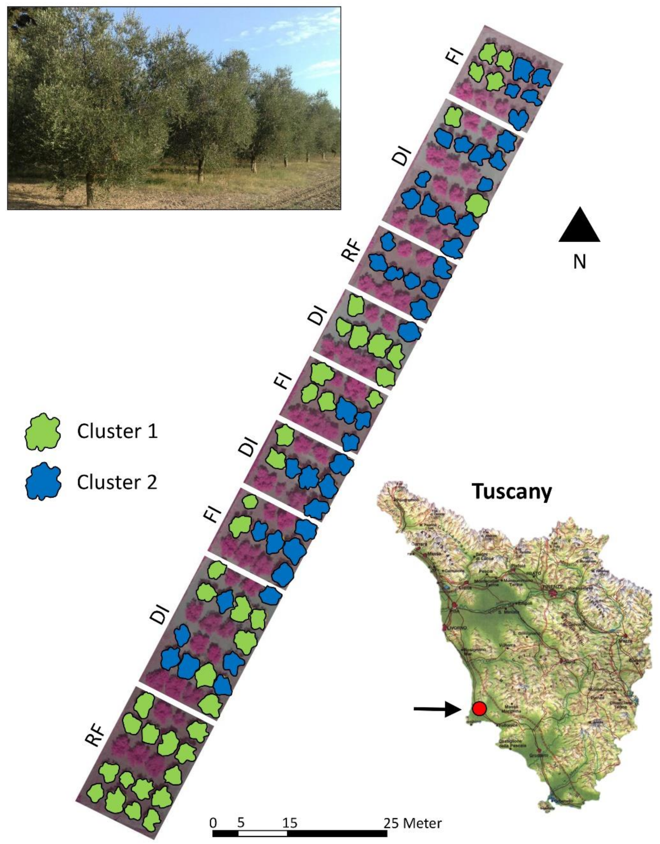
2.1. Plant Material and Site

Experiments were carried out in a high density (513 trees per hectare), 17-year old, irrigated olive orchard at the experimental farm of the University of Pisa, in Venturina (Italy). The orchard included six cultivars, but the work was carried out only on cv. Frantoio, which was the most abundant (61% of the total). A complete description of the plant material and orchard management has been previously published [5,7].
Climatic conditions during the study period were monitored using an iMETOS IMT 300 weather station (Pessl Instruments GmbH, Weiz, Austria). The annual reference evapotranspiration (ET0), calculated according to the Penman-Monteith equation, was 952 mm. Annual and summer (21 June–22 September) precipitations were 809 and 39 mm, respectively. Cultural practices and monitoring of phenological parameters, including the estimation of the full bloom date (DOY 148), were performed as previously reported [5,7].

2.2. Irrigation Management and Measurements

The trees were irrigated using a subsurface drip irrigation system (2.3 L h−1 pressure-compensated drippers spaced at 0.6 m). Irrigation volumes were calculated on the basis of the effective evapotranspiration (ETc), using a crop coefficient (Kc) of 0.55, 0.60 and 0.65 in July, August and September, respectively. The irrigation period lasted from DOY 188 (7 July) to DOY 274 (1 October), during which fully-irrigated (FI) and deficit-irrigated (DI) trees received a total volume of 2160 and 970 m3 ha−1, respectively, whereas the rainfed (RF) ones received only precipitation. Fertigation was used to supply mineral nutrients in spring before irrigation treatments started.
Tree water status was monitored at three dates (DOY 187, DOY 218 and DOY 245) by measuring the stem water potential (SWP) on six trees per irrigation treatment (three trees per each cluster-irrigation combination, as explained in Section 2.5). SWP was measured after blocking transpiration of leaves inserted near the main scaffolds of the tree [47].
Vegetative growth was evaluated as the annual increment in the trunk cross-sectional area (TCSA). The TCSA was calculated from the circumference of the trunk at 0.40 m from the ground, measured on DOY 11 and 356. Immediately before harvest, 100 fruits were randomly sampled from around the canopy of three trees per each cluster-irrigation regime combination to measure mesocarp and endocarp fresh and dry weight. At harvest (DOY 285), each tree was harvested by hand and the final fruit yield was weighed. The oil content of the fruit mesocarp of 20 fruits per tree previously sampled for fresh weight determinations was measured at harvest by nuclear magnetic resonance Oxford MQC-23 analyzer (Oxford Analytical Instruments Ltd., Oxford, UK). The mesocarp was cut in small pieces (2–5 mm) and oven-dried at 70 °C for 48 h. The oil yield of individual trees was calculated as previously reported [48]. Water use efficiency for fruit (WUEf) and oil (WUEo) was calculated as the ratio between fruit yield (dry weight) or oil yield, respectively, and annual ETc within each irrigation treatment.

2.3. Multispectral Imagery Acquisition and Analysis

Images were acquired one day before the beginning of the irrigation differentiation (DOY 187) using a multispectral camera (Tetracam ADC-lite, Tetracam, Inc., Gainesville, FL, USA), mounted on a S1000 UAV octocopter (DJI, Shenzhen, China) able to fly autonomously over a predetermined waypoint. NIR-RG images were recorded in the visible red (R), green (G), and near-infrared (NIR) domain with nominal wavelengths of 520–600, 630–690, and 760–900 nm, respectively.
Images were acquired at noon under clear sky conditions, the flight altitude was 70 m above ground level (AGL), as reported by Caruso et al. [25]. Before the UAV flight, a set of eight ground control points (GCPs) were placed in the orchard and georeferenced using a Leica GS09 real-time kinematic GPS (Leica Geosystems A.G., Heerbrugg, Switzerland). Multispectral images were first mosaicked using Autopano Giga 3.5 Software (Kolor SARL, Challes-les-Eaux, France), then georeferenced and orthorectified using the ground reference points (ArcGIS software, ESRI, Redlands, CA, USA) ad reported by Caruso et al. [25]. The NDVI index [49] was calculated using the map algebra technique implemented in ArcGIS software (ESRI, Redlands, CA, USA) using the following equation:
NDVI = (NIR − RED)/(NIR + RED)
where NIR and RED are the reflectance values in the near-infrared (630–690 nm) and red (760–900 nm) bands, respectively.

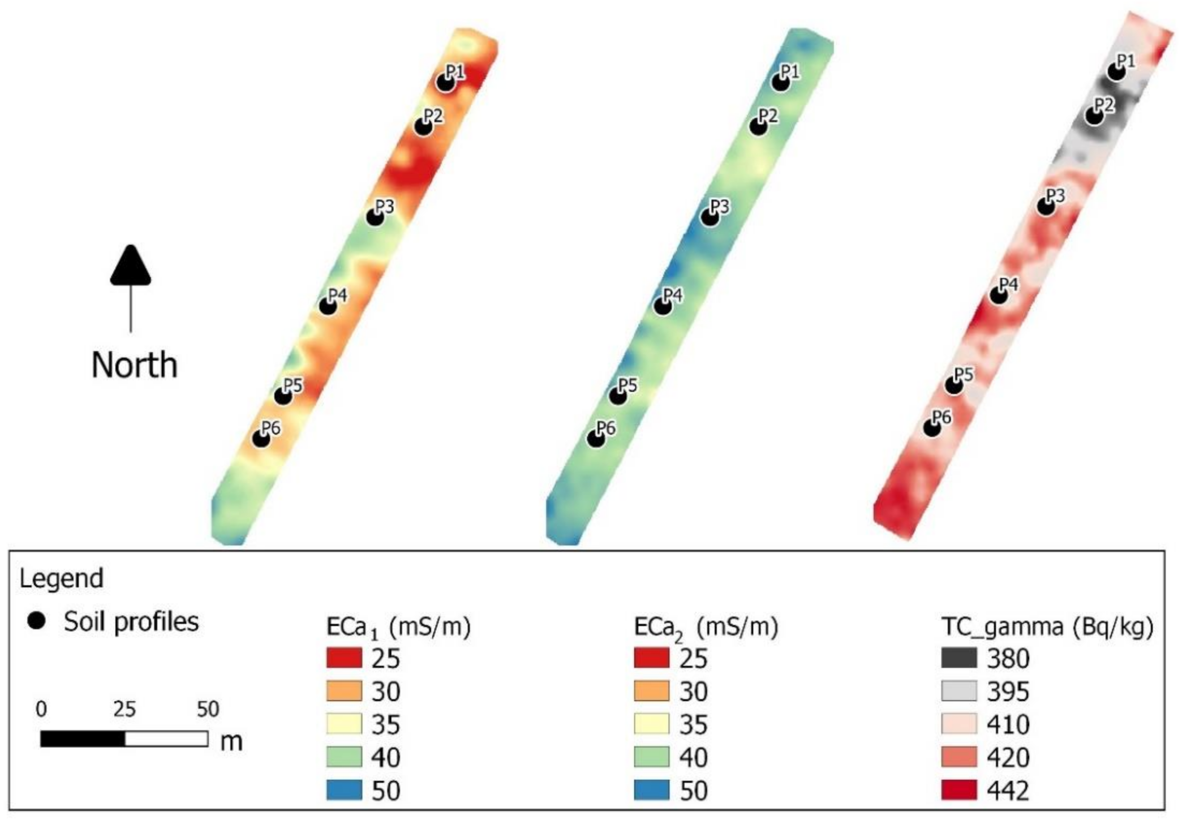
2.4. Proximal Soil Sensing and Soil Analysis

Two different proximal soil sensors (PSS) were used to map soil spatial variability at high resolution. The proximal sensors used were: (i) EM38-Mk2 electromagnetic induction sensor (Geonics Ltd., Mississauga, ON, Canada); (ii) “The Mole”, gamma-ray spectroradiometer (Soil Company, Groningen, The Netherlands). The EM38-Mk2 measures the apparent electrical conductivity (ECa) of the soil at two depth ranges of about 0–0.75 (ECa1) and 0–1.50 m (ECa2) [50]. Soil physical properties, such as texture, stoniness, bulk density [51], soil moisture and water availability [52,53], soil depth [54], as well as organic matter [55] all affect ECa. “The Mole” spectroradiometer continuously measures the natural gamma-ray emission coming from the first 0.3–0.4 m of the soil and rocks, through a Cesium Iodide scintillator crystal [56]. The gamma-ray spectra were analyzed by a Full Spectrum Analysis (FSA), using “The Gamman” software (Medusa Systems, The Netherlands) [22]. This method identifies and deletes data outliers, as well as processes gamma-ray spectrum for calculation of individual nuclide concentrations (40 K, 238 U, 232 Th) and total counts (TC_gamma) in Bq·kg−1. TC_gamma depicts the total count measured by the CsI scintillator for the whole range of energy bands. Proximal gamma-radiometrics has been used to survey topsoil features, such as texture [57], gravel content [22], potassium [58]), and organic carbon [59]. Both the gamma-ray spectroradiometer and EM38-Mk2 were manually driven (without using a tractor or ATV), since the size of the experimental field was relatively small. The sensors were supplied with GPS and rugged PC for data-logging. Soil sensing was performed continuously along each tree row, with the sensors at 0.2 m height above the soil surface, to minimize the signal attenuation. The data were interpolated across the whole area using ordinary kriging (OK), which is widely used or the interpolation of soil proximal sensing data [14,17,19]. The OK parameters, namely lag size, number of lags, and maximum range were selected in order to minimize the estimation error.
Six soil profiles were dug to account for the variability across the field, in terms of proximal soil sensing maps and irrigation management. The soil profiles were described following the international guidelines for soil description [60] and classified according to the Word Reference Base for Soil Resources [61]. Soil samples were collected from several genetic horizons of each soil profile. The samples were air-dried, sieved to 2.0 mm, and analysed for physical and chemical properties using standard laboratory methods. In particular, soil texture was determined by the Micromeritics Sedigraph analyser [62], total organic C (TOC) and total N (TN) were measured by dry combustion with a ThermoFlash 2000 CN soil analyser, after removal of carbonates by HCl 10%. The total equivalent CaCO3 content was calculated from the difference between the total C measured by dry combustion in the untreated soil (mineral C + organic C) and in the HCl-treated soil (organic C). Soil pH was measured potentiometrically in a 1:2.5 soil–water suspension, whereas electrical conductivity was measured in a 1:2 soil–water filtered extract after 2 h shaking and overnight standing. Available water capacity (AWC, in cm cm−1) was calculated for all the soil horizons using the pedotransfer function of Saxton and Rawls [63] implemented in the software SPAW (U.S. Department of Agriculture, Washington D.C., MD, USA).

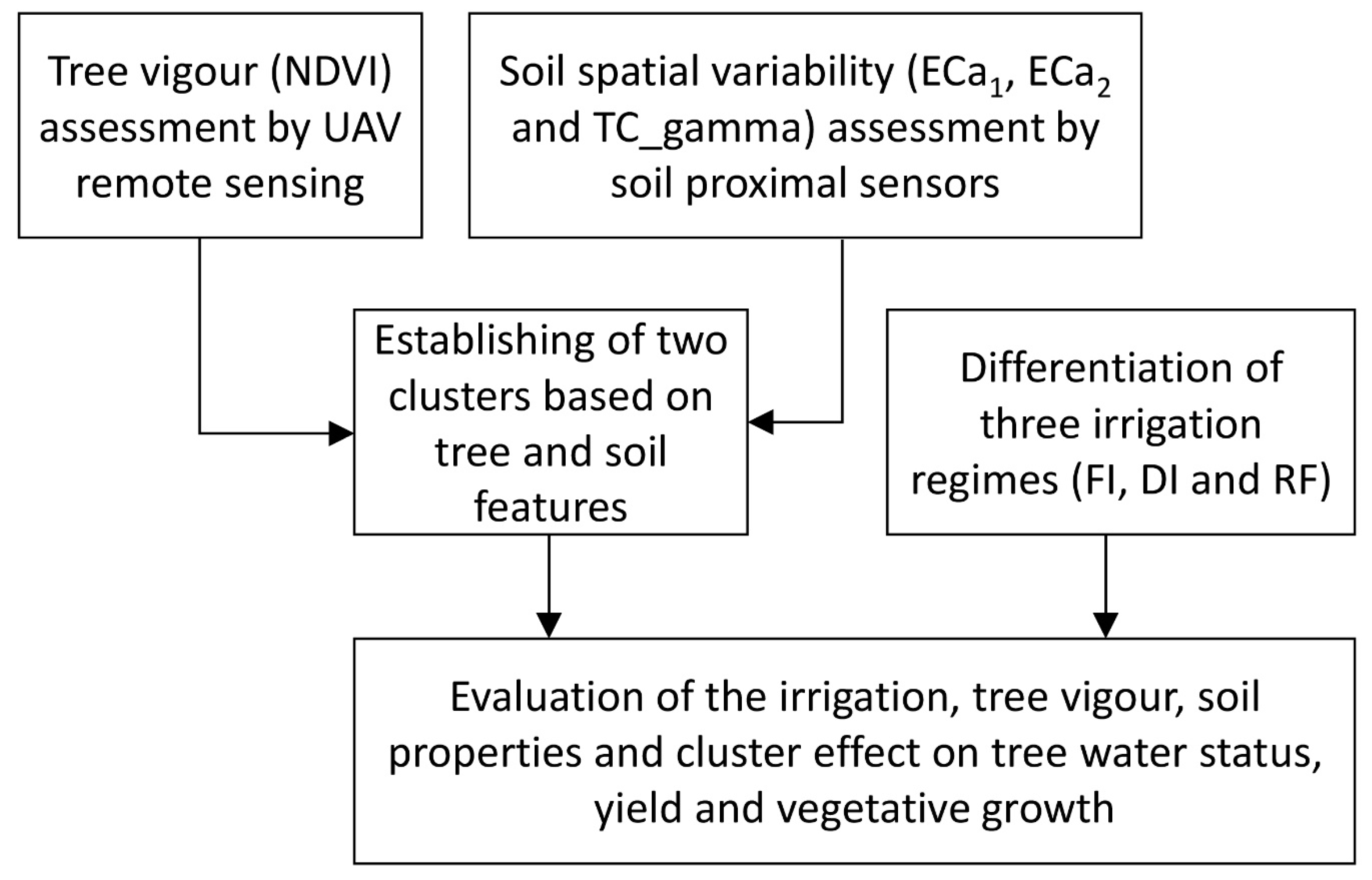
2.5. Experimental Design

The orchard consisted of 12 plots, each containing 12 trees arranged in three rows of four trees, with the only exception of one plot of two rows [5,6]. Three plots were fully irrigated (FI), six plots were deficit irrigated (DI), whereas the remaining three did not receive any irrigation (RF, rainfed) (Figure 1).
The orchard was subdivided into two homogeneous zones (C1 and C2) by k-means clustering, using the Hill-Climbing algorithm [64] of the SAGA-GIS software. The input data to calculate k-means clustering were: ECa1, ECa2, TC_gamma, and NDVI. Such homogeneous zones simulated two prescription areas for site-specific management (in particular precision irrigation) of the olive orchard (Figure 2). The selection of only two clusters was driven by the small surface of the experimental field and by the relatively homogeneous soil.

2.6. Statistical Analysis

The SWP was measured in six trees per irrigation regime (three trees per cluster-irrigation combination) and the means were separated by the least significant differences (LSD p > 0.05) after analysis of variance (ANOVA). An exploratory correlation analysis was performed between NDVI, soil proximal sensing (ECa1, ECa2, TC_gamma), fruit yield, and TCSA increment, to highlight the statistical relationships between the main parameters used for this study. Since most of them showed non-parametric distribution, the Spearman’s ranks correlation test was used. In particular, correlation models within the different irrigation regimes (FI, DI and RF) have been tested by linear regressions. Full factorial ANOVA was carried out to test the effects of the irrigation regimes categorial factors (FI, DI, RF) and homogeneous zones (C1 and C2), as well as the combinations of these factors. Post-hoc LSD Fisher test was used to determine the significant differences between the means of the analysis of variance. To determine the influence of PSS data and NDVI on fruit yield and annual TCSA increment predictions, forward-stepwise multiple regressions were calculated for each irrigation treatment (FI, DI, RF). The independent variables used for the regressions were ECa1, ECa2, TC_gamma, and NDVI. The selection of variables by the forward-stepwise regression was carried out on the basis of F-to enter of 3, to avoid a nonsignificant contribution of some variables in the regression. Statistical analyses were performed with STATISTICA 7.0 (StatSoft Inc., Tulsa, OK, USA).

3. Results

3.1. Proximal Soil Sensing and Profile Description

The soil apparent electrical conductivity ranged between 21.6 and 48.0 mS m−1 in the 0–0.75 m soil profile (ECa1) and between 33.5 and 55.2 mS m−1 considering a deeper soil volume (ECa2, about 0–1.50 m) (Figure 3). The mean values of ECa1 and ECa2 for the entire field were 32.7 and 41.6 mS m−1, respectively. Higher values of ECa were measured on the South and East side of the field.
Low variation of gamma total counts (TC_gamma) was measured by gamma-ray spectroscopy. The values ranged between 376 and 442 Bq kg−1 and indicated a homogeneous mineralogy of the soil parent material. These TC_gamma values were similar to those measured in other soils developed in mixed fluvial deposits of Central Italy [22]. The same study measured values around 250–300 Bq kg−1 in soils developed on calcareous rocks and 550–600 Bq kg−1 in soils on feldspathic sandstones [22].
The maps of radionuclides contribution (40 K, 232 Th, 238 U) showed low variability of the values and a patchworked pattern, which made them unsuitable for further statistical analysis. For this reason, the radionuclide maps were not used for the next step of data analysis. Although the variability of the absolute TC_gamma values was low, the map (Figure 3) showed an evident area with lower values (about 380 Bq kg−1) in the northern part of the field due to surficial stoniness, characterized by about 10–15% of medium and coarse gravel (1–6 cm size). Surficial stoniness was virtually absent in the rest of the orchard.
Two of the six soil profiles were described in this gravelly area (P1 and P2), and they showed the presence of coarse fragments (from 2 to 12%) up to a depth of 0.90 m, whereas the other profiles showed coarse fragments ≤2% only in the Ap horizons. Table 1 shows the two extremes of the soil spatial variability, characterized by the profiles P1 (gravelly area, lower TC_gamma, lower ECa) and P4 (not gravelly area, higher TC_gamma, higher ECa). As a result, the field was characterized by deep (1.5 m) and loamy soils, with a slight increase in clay for illuviation in deep horizons (+6%). Thus, it was classified as Calcaric Luvisol (Loamic, Profondic) according to the international WRB classification [61]. The profiles were similar for other characteristics: loamy texture (tending to loamy-clay in deep Bt horizons), low calcium carbonate content (from 2 to 2.5%), sub-alkaline pH (8–8.3) and absence of salinity. The organic carbon (TOC) of the topsoil (Ap1 horizons) varied from 9 to 37 g kg−1. The TOC of the subsoil horizons varied between 6.5 (deeper Bt horizons) and approximately 10 g kg−1, and the differences between profiles were minimal. Total nitrogen showed the same pattern of TOC, the C/N ratio was relatively stable (approximately 10). Although the soil texture and chemical parameters of the described profiles were quite homogeneous, the different content of the coarse fragments influenced the modelling of the soil available water capacity (AWC).
According to the pedotransfer function of Saxton and Rawls [63], coarse fragments have a negative coefficient, and therefore tend to decrease AWC. For this reason, soil profiles with 10–15% of gravels showed lower AWC (115 mm m−1, for both the profiles) than the other profiles with gravels ≤2% (AWC from 130 to 141 mm m−1). The soil profiles also differed in redoximorphic features, which indicated the depth of temporary waterlogging due to the slow deep drainage (stagnic properties). In particular, the soils of the northern part of the field, characterized by slightly lower ECa and TC_gamma (P1 and P2) showed stagnic properties starting at 1.15 or 1.30 m deep. In contrast, the soils characterized by higher ECa and lower TC, in particular in the southern side of the field, showed stagnic properties starting around 0.90–1.00 m deep. Although the difference of 0.15–0.40 m regarding stagnic properties depth is apparently similar, it could influence the water availability for plants. Water saturation at a depth of 0.9–1.0 m for a certain period of the year does not negatively affect root oxygenation but can provide water for plants for a slightly longer time than soil with deeper stagnic properties.

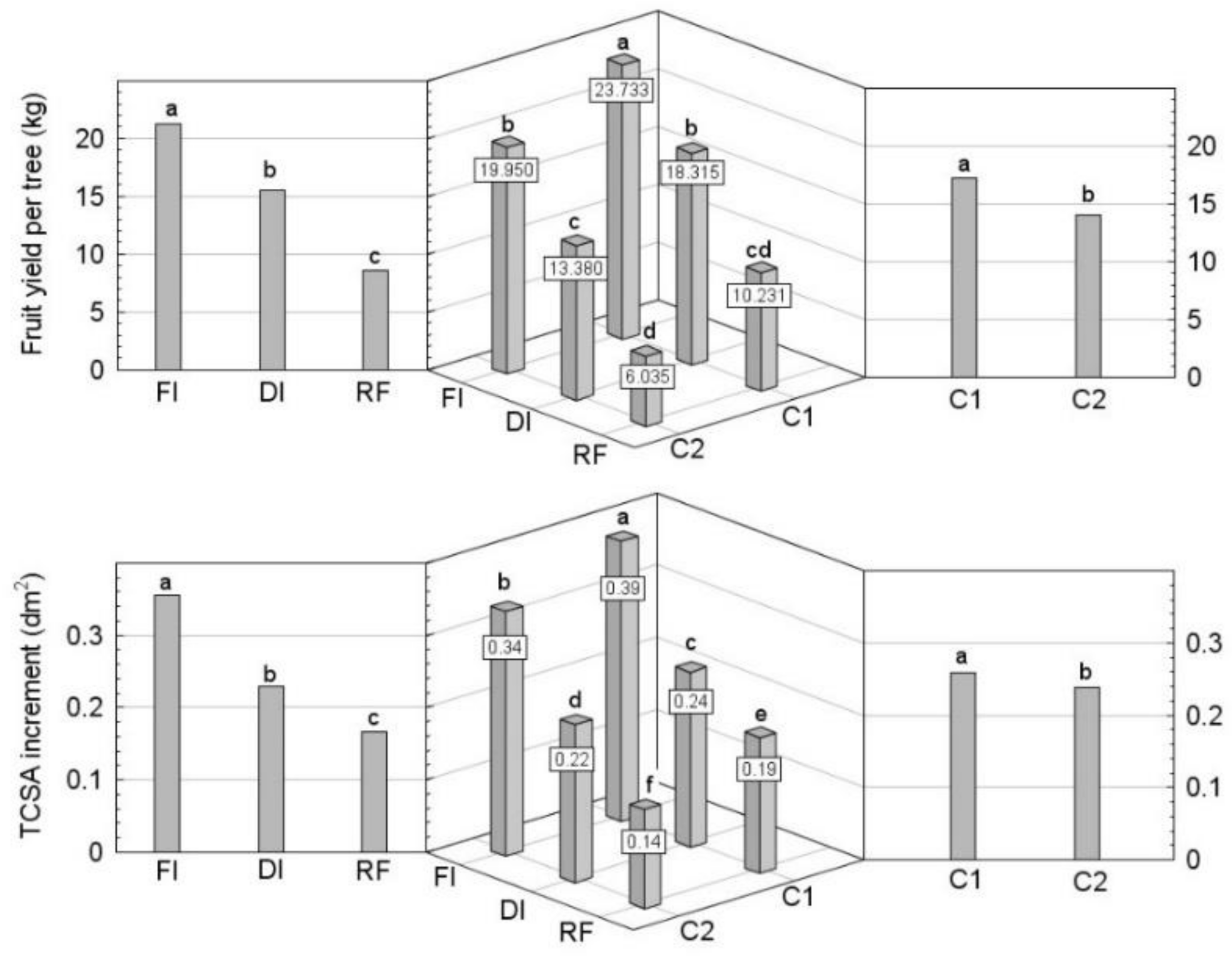
3.2. Irrigation and Cluster Effect on Tree Water Status, Yield and Vegetative Growth

One day after the beginning of the irrigation period (DOY 187) the tree water status was the same across all irrigation regimes and clusters, whereas significant differences in SWP between irrigation treatments were measured at DOY 219 (−1.49, −2.49 and −3.65 MPa in FI, DI and RF trees, respectively) and DOY 259 (−1.57, −2.65 and −3.89 MPa, respectively) (Table 2). Similar trends were measured in both clusters without any significant interaction between irrigation treatment and cluster on tree water status (data not shown).
The fruit yield per tree and the TCSA increment were affected by irrigation, canopy NDVI, and soil ECa1. Irrigation affected both fruit yield (23.890, 15.745 and 8.040 kg per tree in FI, DI, and RF trees, respectively) and the TCSA increment (0.37, 0.23 and 0.16 dm2, respectively) (Figure 4). The two clusters obtained using both remote (NDVI) and proximal (ECa1) sensed indices showed differences in fruit yield (17.259 and 14.003 kg per tree in Cluster 1 and 2, respectively) and annual TCSA increment (0.26 and 0.24 dm2, respectively) (Figure 4). The effect of irrigation on tree productivity and vegetative growth was different between the two clusters. The trees under deficit irrigation grown in the orchard area associated to Cluster 1 showed yields similar to those measured in fully irrigated trees of Cluster 2. Similarly, rainfed trees in Cluster 1 had yields similar to those of trees under deficit irrigation in Cluster 2. The vegetative growth showed significant differences between all the irrigation-cluster combinations (Figure 4).
The highest values of WUEf and WUEo were measured in DI trees in Cluster 1, whereas in Cluster 2 the WUE (both fruit and oil) increased with the amount of water used by the tree (Table 3). Differences in WUE between clusters emerged within each irrigation regime and became increasingly evident as the level of water deficit increased (Table 3).

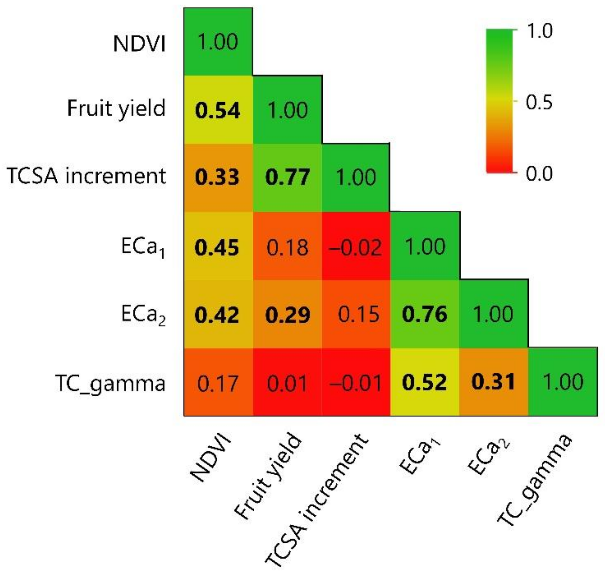
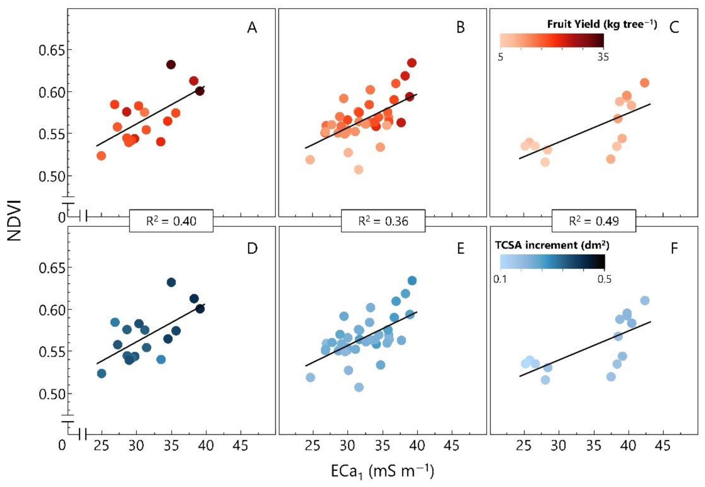
3.3. Comparing Proximal and Remote Sensing Indices against Tree Performances

Significant correlations were evident between NDVI and fruit yield (r = 0.54) and between NDVI and the annual TCSA increment (r = 0.33) when the trees from all irrigation treatments were considered together (Figure 5). Among the soil indices derived from soil sensors, only ECa2 showed a significant, albeit lower, correlation with fruit yield (r = 0.29). Within each irrigation treatment, the highest yield was measured in the most vigorous trees (highest canopy NDVI values) grown in areas with the highest soil ECa1 values, even though a different impact of NDVI and soil ECa1 was observed according to the irrigation treatment (Figure 6).
In particular, the relationship between NDVI and fruit yield and between NDVI and the annual TCSA increment in fully-irrigated trees produced r values of 0.71 and 0.77, respectively, whereas ECa1 showed lower, but still significant correlations (r = 0.62 for both fruit yield and annual TCSA increment) (data not shown). Different results were obtained under rainfed conditions, where the ECa1 showed a higher level of correlation (r = 0.67) with fruit yield than that obtained for the relationship between NDVI and fruit yield (r = 0.54) (data not shown).
A stepwise regression analysis was used to highlight the impact of NDVI, ECa1, ECa2, and TC_gamma on fruit yield and TCSA increment prediction within each irrigation regime (Table 4; Table 5). The regression results show that, under full irrigation, the only variable predictive of yield and TCSA increment was NDVI. Under deficit irrigation, soil spatial variability, determined by ECa maps, also played an important role on yield and TCSA increment, although NDVI remained the most important variable for the prediction of these olive tree parameters. Under rainfed conditions, NDVI was not useful to predict yield, whereas soil features, defined by ECa1 and TC_gamma, on yield, became significant explanatory variables in the multiple regression. On the other hand, for the prediction of TCSA increment, NDVI remained a significant explanatory variable, together with ECa1 and ECa2 under rainfed conditions.

4. Discussion

4.1. Irrigation and Cluster Effect on Tree Performance

Increasing volumes of irrigation increased yield and TCSA of olive trees, in agreement with the large literature on the subject [5,7,8,9,48]. Differences between irrigation treatments were significant regardless of the different soil types in the orchard, as expected. Previous studies on field crops also reported that, although soil properties were major sources of plant variability, water management and fertilization had greater impact on vegetative activity than soil features [34,65]. Precision management of olive orchards aims at optimizing the water use efficiency in terms of fruit (WUEf) and oil (WUEo) yield per liter of consumed water. We determined the impact of the three irrigation regimes on tree productivity in the two clusters identified by the combined use of soil proximal and vegetative remote sensing. The values of WUEo measured in our work were much higher than those measured by Fernandes-Silva et al. [9] in a similar experiment carried out in Portugal (WUEo of 0.19, 0.16 and 0.07 g L−1 for T2-100% ETc, T1-30% ETc and T0-rainfed, respectively), but similar to those reported by Iniesta et al. [8] (WUEo of 0.24 and 0.30 for full and sustained deficit irrigation, respectively). We showed differences in either WUEf or WUEo within the orchard. The higher tree productivity measured in Cluster 1 also resulted in a higher WUEf (0.90) and WUEo (0.32) compared to Cluster 2 (0.67 and 0.27 for WUEf and WUEo, respectively). In particular, in Cluster 1 the WUEf and WUEo of FI trees was 0.98 and 0.39, respectively, whereas in Cluster 2 the trees subjected to the same irrigation regime showed values of 0.90 and 0.36 for the same parameters, respectively. Differences in WUEf and WUEo in the two clusters were more evident under deficit irrigation (WUEf and WUEo of 1.06 and 0.38, respectively, in Cluster 1, and 0.72 and 0.31 in Cluster 2), and rainfed conditions (WUEf and WUEo of 0.66 and 0.21 g L−1, respectively, in Cluster 1, and 0.40 and 0.15 g L−1 in Cluster 2), indicating the increasing impact of the cluster characteristics on tree productivity as irrigation volumes decreased. In a recent study carried out in a high density olive orchard the two management zones identified using a similar approach (combining proximal and remote sensing) showed significant differences in fruit yield only in one out of three years [46]. The authors reported that the lack of differences in those two years was due to a different irrigation management (timing and amount of the applied water) in the two zones.

4.2. Comparing Proximal and Remote Sensing Indices against Tree Performance

The ability of proximal and remote sensing in estimating tree growth and yield has been poorly investigated in olive growing so far. Few previous studies used UAV imagery to estimate fruit yield and vegetative growth of olive trees [25,26,32,33]. In the current work, we observed a general (all irrigation treatments) linear relationship between NDVI and fruit yield (r = 0.54), similarly to previous findings in a hedgerow olive orchard [26]. In that same study, there was no relationship between NDVI and fruit yield in the year when abiotic (spring frost) and biotic (olive fruit fly) factors dramatically affected final fruit yield [26]. A specific response to location and growing season in the NDVI-fruit yield relationship also appeared when results obtained in similar experiments were compared [32,33], highlighting the limit of the fruit yield prediction carried out several months before harvest. A lower level of correlation (r = 0.33) was observed between NDVI and the TCSA increment when all the trees from the three irrigation treatments were considered together. In a previous study carried out using the same cultivar, Caruso et al. [25] reported a combined effect of tree water status and canopy NDVI on the final TCSA increment. Soil indices derived by proximal sensing (ECa1, ECa2, and TC_gamma) were less able to predict fruit yield (r = 0.18, 0.29 and 0.01, respectively) and TCSA increment (0.02, 0.15 and 0.01) when all irrigation treatments were considered together. A wide range of correlation coefficients between ECa and fruit yield (R2 comprised between 0.01 and 0.94) was reported in previous studies carried out on different cultivars of apple trees [44,66]. In a previous study carried out in a commercial olive orchard, significant relationships between the soil characteristics (organic matter, B and Ca) derived by a systematic sampling grid and the fruit yield were measured only in one of the two experimental years [67].
To discriminate the impact of proximally (soil) and remotely (tree) determined indices on tree parameters (yield and TCSA increment) under different irrigation regimes we used a stepwise multiple regression analysis. Under full irrigation conditions, the NDVI was the only variable able to describe the variability in fruit yield and vegetative growth, whereas under rainfed conditions the soil parameters (ECa1, ECa2 and TC_gamma) were identified as the only factors affecting yield. Interestingly, under deficit irrigation, both tree (NDVI) and soil (ECa1 and ECa2) parameters were identified as factors contributing to the measured yield parameters. In a similar study in an irrigated vineyard, Terrón et al. [68] also reported high correlations between NDVI and soil ECa, but such a relationship was strongly dependent on the growing season and the irrigation regime. Therefore, the role of soil spatial variability was much more important as water deficit became more severe, whereas in cases when water availability was high due to rains or irrigation, the variability of soil characteristics played a less important role on vegetative growth. Priori et al. [69] showed that the effects of soil features on grape and wine peculiarities were much more evident during dry years, whereas rainy summers tended to hide this variability in a rainfed vineyard.

5. Conclusions

We showed that remote and proximal sensing technologies allowed to determine that the effect of different irrigation regimes on tree performance and WUE depended on the location within the orchard (Cluster 1 and Cluster 2). The second finding of this study concerns the major role of tree vigour in determining the final fruit yield under optimal soil water availability, whereas soil features become the most important factors under rainfed conditions. Since water availability in the Mediterranean climate is becoming increasingly limited, this information may be crucial to optimize the water management through site-specific irrigation protocols. They should be considered preliminary, as the investigation was done over one growing season only. Furthermore, since olive trees are subject to alternate bearing, long-term studies are needed to evaluate the stability of the orchard zone effects on yield and tree growth in high- (“on-year”) and low- (“off-year”) yield crop years.

Author Contributions

G.C.: conceptualization, investigation, methodology, formal analysis, resources, software, writing—original draft and editing. G.P.: investigation, data curation, formal analysis, software, writing—review and editing. R.G.: resources, supervision, validation and writing—review. S.P.: conceptualization, investigation, methodology, formal analysis, resources, software and writing—original draft. All authors have read and agreed to the published version of the manuscript.

Funding

This research received no external funding.

Institutional Review Board Statement

Not applicable.

Informed Consent Statement

Not applicable.

Data Availability Statement

Not applicable.

Acknowledgments

The irrigation system was kindly supplied by Netafim Italia.

Conflicts of Interest

The authors declare no conflict of interest.

References

  1. Norrant, C.; Douguédroit, A. Monthly and daily precipitation trends in the Mediterranean (1950–2000). Theor. Appl. Climatol. 2006, 83, 89–106. [Google Scholar] [CrossRef]
  2. Guiot, J.; Cramer, W. Climate change: The 2015 Paris Agreement thresholds and Mediterranean basin ecosystems. Science 2016, 354, 465–468. [Google Scholar] [CrossRef] [PubMed]
  3. IPCC; Mirzabaev, A.; Wu, J.; Evans, J.; García-Oliva, F.; Hussein, I.A.G.; Iqbal, M.H.; Kimutai, J.; Knowles, T.; Meza, F.; et al. Desertification. In Climate Change and Land: An IPCC Special Report on Climate Change, Desertification, Land Degradation, Sustainable Land Management, Food Security, and Greenhouse Gas Fluxes in Terrestrial Ecosystems; IPCC: New York, NY, USA, 2019. [Google Scholar]
  4. Spinoni, J.; Naumann, G.; Vogt, J.; Barbosa, P. Meteorological Droughts in Europe: Events and Impacts: Past Trends and Future Projections; EUR 27748; Publications Office of the European Union: Luxembourg, 2016. [Google Scholar]
  5. Caruso, G.; Rapoport, H.F.; Gucci, R. Long-term evaluation of yield components of young olive trees during the onset of fruit production under different irrigation regimes. Irrig. Sci. 2013, 31, 37–47. [Google Scholar] [CrossRef] [Green Version]
  6. Caruso, G.; Gucci, R.; Urbani, S.; Esposto, S.; Taticchi, A.; Di Maio, I.; Selvaggini, R.; Servili, M. Effect of different irrigation volumes during fruit development on quality of virgin olive oil of cv. Frantoio. Agric. Water Manag. 2014, 134, 94–103. [Google Scholar] [CrossRef]
  7. Gucci, R.; Caruso, G.; Gennai, C.; Esposto, S.; Urbani, S.; Servili, M. Fruit growth, yield and oil quality changes induced by deficit irrigation at different stages of olive fruit development. Agric. Water Manag. 2019, 212, 88–98. [Google Scholar] [CrossRef]
  8. Iniesta, F.; Testi, L.; Orgaz, F.; Villalobos, F.J. The effects of regulated and continuous deficit irrigation on the water use, growth and yield of olive trees. Eur. J. Agron. 2009, 30, 258–265. [Google Scholar] [CrossRef]
  9. Fernandes-Silva, A.A.; Ferreira, T.C.; Correia, C.M.; Malheiro, A.C.; Villalobos, F.J. Influence of different irrigation regimes on crop yield and water use efficiency of olive. Plant Soil 2010, 333, 35–47. [Google Scholar] [CrossRef] [Green Version]
  10. Marra, F.P.; Marino, G.; Marchese, A.; Caruso, T. Effects of different irrigation regimes on a super-high-density olive grove cv. “Arbequina”: Vegetative growth, productivity and polyphenol content of the oil. Irrig. Sci. 2016, 34, 313–325. [Google Scholar] [CrossRef]
  11. Brouder, S.M.; Hofmann, B.S.; Morris, D.K. Mapping soil pH: Accuracy of common soil sampling strategies and estimation techniques. Soil Sci. Soc. Am. J. 2005, 69, 427–442. [Google Scholar] [CrossRef]
  12. Khosla, R.; Alley, M.M. Soil-specific nitrogen management on mid-Atlantic coastal plain soils. Better Crop. 1999, 83, 6–7. [Google Scholar]
  13. Moral, F.J.; Rebollo, F.J.; Campillo, C.; Serrano, J.M. Using an objective and probabilistic model to delineate homogeneous zones in hedgerow olive orchards. Soil Till. Res. 2019, 194, 104308. [Google Scholar] [CrossRef]
  14. Rodrigues, F.A., Jr.; Bramley, R.G.V.; Gobbett, D.L. Proximal soil sensing for precision agriculture: Simultaneous use of electromagnetic induction and gamma radiometrics in contrasting soils. Geoderma 2015, 243, 183–195. [Google Scholar] [CrossRef]
  15. Munnaf, M.A.; Haesaert, G.; Mouazen, A.M. Map-based site-specific seeding of seed potato production by fusion of proximal and remote sensing data. Soil Till. Res. 2021, 206, 104801. [Google Scholar] [CrossRef]
  16. Darra, N.; Psomiadis, E.; Kasimati, A.; Anastasiou, A.; Anastasiou, E.; Fountas, S. Remote and proximal sensing-derived spectral indices and biophysical variables for spatial variation determination in vineyards. Agronomy 2021, 11, 741. [Google Scholar] [CrossRef]
  17. Corwin, D.L.; Lesch, S.M. Application of soil electrical conductivity to precision agriculture: Theory, principles, and guidelines. Agron. J. 2003, 95, 455–471. [Google Scholar] [CrossRef]
  18. Visconti, F.; De Paz, J.M. Sensitivity of soil electromagnetic induction measurements to salinity, water content, clay, organic matter and bulk density. Precis. Agric. 2021, 22, 1559–1577. [Google Scholar] [CrossRef]
  19. Priori, S.; Martini, E.; Andrenelli, M.C.; Magini, S.; Agnelli, A.E.; Bucelli, P.; Biagi, M.; Pellegrini, S.; Costantini, E.A.C. Improving wine quality through harvest zoning and combined use of remote and soil proximal sensing. Soil Sci. Soc. Am. J. 2013, 77, 1338–1348. [Google Scholar] [CrossRef]
  20. Pedrera-Parrilla, A.; Martínez, G.; Espejo-Pérez, A.J.; Gómez, J.A.; Giráldez, J.V.; Vanderlinden, K. Mapping impaired olive tree development using electromagnetic induction surveys. Plant Soil 2014, 384, 381–400. [Google Scholar] [CrossRef] [Green Version]
  21. Martinez, G.; Huang, J.; Vanderlinden, K.; Giraldez, J.V.; Triantafilis, J. Potential to predict depth-specific soil–water content beneath an olive tree using electromagnetic conductivity imaging. Soil Use Manag. 2018, 34, 236–248. [Google Scholar] [CrossRef]
  22. Priori, S.; Bianconi, N.; Costantini, E.A.C. Can γ-radiometrics predict soil textural data and stoniness in different parent materials? A comparison of two machine-learning methods. Geoderma 2014, 226–227, 354–364. [Google Scholar] [CrossRef]
  23. Heggemann, T.; Welp, G.; Amelung, W.; Angst, G.; Franz, S.O.; Koszinski, S.; Schmidt, K.; Pätzold, S. Proximal gamma-ray spectrometry for site-independent in situ prediction of soil texture on ten heterogeneous fields in Germany using support vector machines. Soil Till. Res. 2017, 168, 99–109. [Google Scholar] [CrossRef]
  24. De Mello, D.C.; Demattê, J.A.M.; De Oliveira Mello, F.A.; Poppiel, R.R.; Silvero, N.E.; Safanelli, J.L.; Barros e Souza, A.; Di Loreto Di Raimo, L.A.; Rizzo, R.; Bispo Resende, M.E.; et al. Applied gamma-ray spectrometry for evaluating tropical soil processes and attributes. Geoderma 2021, 381, 114736. [Google Scholar] [CrossRef]
  25. Caruso, G.; Zarco-Tejada, P.J.; Gonzalez-Dugo, V.; Moriondo, M.; Tozzini, L.; Palai, G.; Rallo, G.; Hornero, A.; Primicerio, J.; Gucci, R. High-resolution imagery acquired from an unmanned platform to estimate biophysical and geometrical parameters of olive trees under different irrigation regimes. PLoS ONE 2019, 14, e0210804. [Google Scholar] [CrossRef] [PubMed] [Green Version]
  26. Caruso, G.; Palai, G.; Marra, F.P.; Caruso, T. High-resolution UAV imagery for field olive (Olea europaea L.) phenotyping. Horticulturae 2021, 7, 258. [Google Scholar] [CrossRef]
  27. Padua, L.; Adão, T.; Sousa, A.; Peres, E.; Sousa, J.J. Individual grapevine analysis in a multi-temporal context using UAV-based multi-sensor imagery. Remote Sens. 2020, 12, 139. [Google Scholar] [CrossRef] [Green Version]
  28. Torres-Sánchez, J.; López-Granados, F.; Serrano, N.; Arquero, O.; Peña, J. High-throughput 3-D monitoring of agricultural-tree plantations with unmanned aerial vehicle (UAV) technology. PLoS ONE 2015, 10, e0130479. [Google Scholar] [CrossRef] [PubMed] [Green Version]
  29. Zarco-Tejada, P.J.; Diaz-Varela, R.; Angileri, V.; Loudjani, P. Tree height quantification using very high resolution imagery acquired from an unmanned aerial vehicle (UAV) and automatic 3D photo-reconstruction methods. Eur. J. Agron. 2014, 55, 89–99. [Google Scholar] [CrossRef]
  30. Peña-Barragán, J.M.; Jurado-Expósito, M.; López-Granados, F.; Atenciano, S.; Sánchez-de la Orden, M.; García-Ferrer, A.; García-Torres, L. Assessing land-use in olive groves from aerial photographs. Agric. Ecosyst. Environ. 2004, 103, 117–122. [Google Scholar] [CrossRef]
  31. Noori, O.; Panda, S.S. Site-specific management of common olive: Remote sensing, geospatial, and advanced image processing applications. Comput. Electron. Agric. 2016, 127, 680–689. [Google Scholar] [CrossRef]
  32. Sola-Guirado, R.R.; Castillo-Ruiz, F.J.; Jiménez-Jiménez, F.; Blanco-Roldan, G.L.; Castro-Garcia, S.; Gil-Ribes, J.A. Olive actual “on year” yield forecast tool based on the tree canopy geometry using UAS imagery. Sensors 2017, 17, 1743. [Google Scholar] [CrossRef] [Green Version]
  33. Stateras, D.; Kalivas, D. Assessment of olive tree canopy characteristics and yield forecast model using high resolution UAV imagery. Agriculture 2020, 10, 385. [Google Scholar] [CrossRef]
  34. De Benedetto, D.; Castrignano, A.; Diacono, M.; Rinaldi, M.; Ruggieri, S.; Tamborrino, R. Field partition by proximal and remote sensing data fusion. Biosyst. Eng. 2013, 114, 372–383. [Google Scholar] [CrossRef]
  35. Ortega-Blu, R.; Molina-Roco, M. Evaluation of vegetation indices and apparent soil electrical conductivity for site-specific vineyard management in Chile. Precis. Agric. 2016, 17, 434–450. [Google Scholar] [CrossRef]
  36. Panda, S.S.; Hoogenboom, G.; Paz, J.O. Remote sensing and geospatial technological applications for site-specific management of fruit and nut crops: A review. Remote Sens. 2010, 2, 1973–7997. [Google Scholar] [CrossRef] [Green Version]
  37. Bonfante, A.; Agrillo, A.; Albrizio, R.; Basile, A.; Buonomo, R.; De Mascellis, R.; Terribile, F. Functional homogeneous zones (fHZs) in viticultural zoning procedure: An Italian case study on Aglianico vine. Soil 2015, 1, 427–441. [Google Scholar] [CrossRef] [Green Version]
  38. Tardaguila, J.; Diago, M.P.; Priori, S.; Oliveira, M. Mapping and managing vineyard homogeneous zones through proximal geoelectrical sensing. Arch. Agron. Soil Sci. 2018, 64, 409–418. [Google Scholar] [CrossRef]
  39. Bahat, I.; Netzer, Y.; Grünzweig, J.M.; Alchanatis, V.; Peeters, A.; Goldshtein, E.; Ohana-Levi, N.; Ben-Gal, A.; Cohen, Y. In-season interactions between vine vigor, water status and wine quality in terrain-based management-zones in a ‘Cabernet Sauvignon’ vineyard. Remote Sens. 2021, 13, 1636. [Google Scholar] [CrossRef]
  40. Caruso, G.; Tozzini, L.; Rallo, G.; Primicerio, J.; Moriondo, M.; Palai, G.; Gucci, R. Estimating biophysical and geometrical parameters of grapevine canopies (‘Sangiovese’) by an unmanned aerial vehicle (UAV) and VIS-NIR cameras. Vitis 2017, 56, 63–70. [Google Scholar] [CrossRef]
  41. Serrano, J.; Shahidian, S.; Marques da Silva, J.; Paixão, L.; Calado, J.; de Carvalho, M. Integration of soil electrical conductivity and indices obtained through satellite imagery for differential management of pasture fertilization. AgriEngineering 2019, 1, 567–585. [Google Scholar] [CrossRef] [Green Version]
  42. Bellvert, J.; Mata, M.; Vallverdú, X.; Paris, C.; Marsal, J. Optimizing precision irrigation of a vineyard to improve water use efficiency and profitability by using a decision-oriented vine water consumption model. Precis. Agric. 2021, 22, 319–341. [Google Scholar] [CrossRef]
  43. Aggelopoulou, K.; Wulfsohn, D.; Fountas, S.; Nanos, G.; Gemtos, T.; Blackmore, S. Spatial variability of yield and quality in an apple orchard. Precis. Agric. 2010, 11, 538–556. [Google Scholar] [CrossRef]
  44. Türker, U.; Talebpour, B.; Yegül, U. Determination of the relationship between apparent soil electrical conductivity with pomological properties and yield in different apple varieties. Agriculture 2011, 98, 307–314. [Google Scholar]
  45. Uribeetxebarria, A.; Daniele, E.; Escolà, A.; Arnó, J.; Martinez-Casasnovas, J.A. Spatial variability in orchards after land transformation: Consequences for precision agriculture practices. Sci. Total Environ. 2018, 635, 343–352. [Google Scholar] [CrossRef] [PubMed]
  46. Millán, S.; Moral, F.J.; Prieto, M.H.; Pérez-Rodríguez, J.M.; Campillo, C. Mapping soil properties and delineating management zones based on electrical conductivity in a hedgerow olive grove. Trans. ASABE 2019, 62, 749–760. [Google Scholar] [CrossRef]
  47. McCutchan, H.; Shackel, K.A. Stem-water potential as a sensitive indicator of water stress in prune trees (Prunus domestica L. cv. French). J. Am. Soc. Hortic. Sci. 1992, 117, 607–611. [Google Scholar] [CrossRef] [Green Version]
  48. Gucci, R.; Lodolini, E.; Rapoport, H.F. Productivity of olive trees with different water status and crop load. J. Hortic. Sci. Biotechnol. 2007, 82, 648–656. [Google Scholar] [CrossRef]
  49. Rouse, J.W., Jr.; Haas, R.H.; Deering, D.W.; Schell, J.A.; Harlan, J.C. Monitoring the Vernal Advancement and Retrogradation (Greenwave Effect) of Natural Vegetation; NASA/GSFC Type III Final Report; NASA: Greenbelt, MD, USA, 1974; p. 371. [Google Scholar]
  50. McNeill, J.D. Use of electromagnetic methods for groundwater studies. In Geotechnical an Environmental Geophysics: Volume I: Review and Tutorial; Society of Exploration Geophysicists: Houston, TX, USA, 1990; pp. 191–218. [Google Scholar]
  51. Nocco, M.A.; Ruark, M.D.; Kucharik, C.J. Apparent electrical conductivity predicts physical properties of coarse soils. Geoderma 2019, 335, 1–11. [Google Scholar] [CrossRef]
  52. Martini, E.; Wollschläger, U.; Musolff, A.; Werban, U.; Zacharias, S. Principal component analysis of the spatiotemporal pattern of soil moisture and apparent electrical conductivity. Vadose Zone J. 2017, 16, 1–12. [Google Scholar] [CrossRef]
  53. Farzamian, M.; Paz, M.C.; Paz, A.M.; Castanheira, N.L.; Gonçalves, M.C.; Monteiro Santos, F.A.; Triantafilis, J. Mapping soil salinity using electromagnetic conductivity imaging—A comparison of regional and location-specific calibrations. Land Degrad. Dev. 2019, 30, 1393–1406. [Google Scholar] [CrossRef]
  54. Priori, S.; Fantappiè, M.; Magini, S.; Costantini, E.A.C. Using the ARP-03 for high-resolution mapping of calcic horizons. Int. Agrophys. 2013, 27, 313–321. [Google Scholar] [CrossRef] [Green Version]
  55. Huang, J.; Pedrera-Parrilla, A.; Vanderlinden, K.; Taguas, E.V.; Gómez, J.A.; Triantafilis, J. Potential to map depth-specific soil organic matter content across an olive grove using quasi-2d and quasi-3d inversion of DUALEM-21 data. Catena 2017, 152, 207–217. [Google Scholar] [CrossRef]
  56. Van Egmond, F.M.; Loonstra, E.H.; Limburg, J. Gamma ray sensor for topsoil mapping: The Mole. In Proximal Soil Sensing; Springer: Dordrecht, The Netherlands, 2010; pp. 323–332. [Google Scholar]
  57. Coulouma, G.; Caner, L.; Loonstra, E.H.; Lagacherie, P. Analysing the proximal gamma radiometry in contrasting Mediterranean landscapes: Towards a regional prediction of clay content. Geoderma 2016, 266, 127–135. [Google Scholar] [CrossRef]
  58. Kassim, A.M.; Nawar, S.; Mouazen, A.M. Potential of on-the-go gamma-ray spectrometry for estimation and management of soil potassium site specifically. Sustainability 2021, 13, 661. [Google Scholar] [CrossRef]
  59. Dierke, C.; Werban, U. Relationships between gamma-ray data and soil properties at an agricultural test site. Geoderma 2013, 199, 90–98. [Google Scholar] [CrossRef]
  60. Jahn, R.; Blume, H.P.; Asio, V.B.; Spaargaren, O.; Schad, P. Guidelines for Soil Description; FAO: Rome, Italy, 2006. [Google Scholar]
  61. IUSS Working Group WRB. World Reference Base for Soil Resources 2014, Update 2015. International Soil Classification System for Naming Soils and Creating Legends for Soil Maps. World Soil Resources Reports No. 106; FAO: Rome, Italy, 2015. [Google Scholar]
  62. Andrenelli, M.C.; Fiori, V.; Pellegrini, S. Soil particle-size analysis up to 250 μm by X-ray granulometer: Device set-up and regressions for data conversion into pipette equivalent values. Geoderma 2013, 192, 380–393. [Google Scholar] [CrossRef]
  63. Saxton, K.E.; Rawls, W.J. Soil water characteristic estimates by texture and organic matter for hydrologic solutions. Soil Sci. Soc. Am. J. 2006, 70, 1569–1578. [Google Scholar] [CrossRef] [Green Version]
  64. Rubin, J. Optimal classification into groups: An approach for solving the taxonomy problem. J. Theor. Biol. 1967, 15, 103–144. [Google Scholar] [CrossRef]
  65. Basso, B.; Ritchie, J.T.; Cammarano, D.; Sartori, L. A strategic and tactical management approach to select optimal N fertilizer rates for wheat in a spatially variable field. Eur. J. Agron. 2011, 35, 215–222. [Google Scholar] [CrossRef]
  66. Manfrini, L.; Corelli Grappadelli, L.; Morandi, B.; Losciale, P.; Taylor, J. Innovative approaches to orchard management: Assessing the variability in yield and maturity in a ‘Gala’ apple orchard using a simple management unit modeling approach. Eur. J. Hortic. Sci. 2020, 85, 211–218. [Google Scholar] [CrossRef]
  67. Fountas, S.; Aggelopoulou, K.; Bouloulis, C.; Nanos, G.D.; Wulfsohn, D.; Gemtos, T.A.; Paraskevopoulos, A.; Galanis, M. Site-specific management in an olive tree plantation. Precis. Agric. 2011, 12, 179–195. [Google Scholar] [CrossRef]
  68. Terrón, J.M.; Blanco, J.; Moral, F.J.; Mancha, L.A.; Uriarte, D.; Marques da Silva, J.R. Evaluation of vineyard growth under four irrigation regimes using vegetation and soil on-the-go sensors. Soil 2015, 1, 459–473. [Google Scholar] [CrossRef] [Green Version]
  69. Priori, S.; Pellegrini, S.; Perria, R.; Puccioni, S.; Storchi, P.; Valboa, G.; Costantini, E.A. Scale effect of terroir under three contrasting vintages in the Chianti Classico area (Tuscany, Italy). Geoderma 2019, 334, 99–112. [Google Scholar] [CrossRef]
Figure 1. False colour orthophoto of the olive orchard located at the experimental farm of the Department of Agriculture Food and Environment of the University of Pisa (43°10′ N; 10°36′ E). The canopies of the olive trees cv. Frantoio are in green (Cluster 1) or light blue (Cluster 2). The trees of other cultivars were not used in the experiment.
Applsci 12 01309 g001
Figure 2. Flow chart of the experiment. Legend: NDVI, normalized difference vegetation index; ECa1 and ECa2, apparent electrical conductivity at 0–0.75 and 0.75–1.50 m soil depth; TC_gamma, total count gamma ray; FI, full irrigation; DI, deficit irrigation; RF, rainfed conditions.
Applsci 12 01309 g002
Figure 3. The maps obtained by the soil proximal sensing, and the location of the soil profiles (P1–P6, black dots). The left and central maps showed the apparent electrical conductivity (ECa) at two reference depths, about 0–0.75 (ECa1) and 0–1.50 m (ECa2). The map on the right showed the gamma-ray total counts (TC_gamma) of the topsoil, about 0–0.30 m. The lower values of TC_gamma in the northern part of the field correspond to the area with higher surficial stoniness.
Applsci 12 01309 g003
Figure 4. Fruit yield and trunk cross sectional area (TCSA) increment in olive trees subjected to different irrigation regimes (Full irrigation, FI; deficit irrigation, DI; rainfed conditions, RF) and located in different orchard zones (Cluster 1, C1; Cluster 2, C2). Histograms represent the average of 18 (FI), 40 (DI), 15 (RF), 33 (C1), 39 (C2), 7 (FI-C1), 11 (FI-C2), 17 (DI-C1), 23 (DI-C2), 9 (RF-C1), 6 (RF-C2) trees per each irrigation treatment and cluster combination. Different letters indicate significant differences of LSD test after ANOVA (p < 0.05).
Applsci 12 01309 g004
Figure 5. Nonparametric correlation coefficients (Spearman’s ranks) between NDVI, tree parameters (fruit yield and annual TCSA increment) and soil indices (ECa1, ECa2 and TC_gamma) derived by proximal sensing sensors at the experimental site. In bold, the coefficient significant for p < 0.01 (n = 75, all irrigation treatments).
Applsci 12 01309 g005
Figure 6. The relationship between soil ECa1 and the NDVI of trees grown in the soil area under full irrigation (A,D), deficit irrigation (B,E), and rainfed conditions (C,F). Each point represents one tree (and the respective allocated soil area). Coefficients of determination were calculated within each irrigation treatment. Regression equations: NDVI = 0.42 + 0.005 ECa1 (A,D); NDVI = 0.44 + 0.004 ECa1 (B,F); NDVI = 0.44 + 0.003 ECa1 (C,F).
Applsci 12 01309 g006
Table 1. Description of the benchmark profiles which defined the two areas of the field, gravelly (P1) and not gravelly (P4). Legend: Ap1, surface horizon subjected to ploughing; Ap2, sub-surface horizon interested by deep ploughing; Bt, B horizon with clay illuviation process; Btg, B horizon with clay illuviation process and redoximorphic mottles due to temporary waterlogging (stagnic properties); CF, Coarse fragments; SOC, Soil Organic Carbon; TN, Total nitrogen; AWC, Available Water Capacity.
Cluster 1
(Profile 1)
Soil Horizons
Ap1Ap2BtBtg
Depth (m)0.80.401.001.50
Clay (dag kg−1)13.922.517.722.1
Silt (dag kg−1)45.533.244.439.3
Sand (dag kg−1)40.644.337.938.6
CF (%vol)2200
CaCO3 tot (dag kg−1)2.42.52.32.1
SOC (dag kg−1)31.411.09.07.2
TN (g kg−1)24.49.89.77.7
AWC (mm)12458470
Cluster 2Soil Horizons
(Profile 4)Ap1Ap2BtBtg
Depth (m)0.100.350.901.15
Clay (dag kg−1)18.416.116.824.7
Silt (dag kg−1)37.335.436.935.6
Sand (dag kg−1)44.348.546.339.7
CF (%vol)121250
CaCO3 tot (dag kg−1)2.42.32.32.3
SOC (dag kg−1)9.013.19.06.8
TN (g kg−1)9.113.08.97.5
AWC (mm)11286633
Table 2. Stem water potential measured on olive trees grown in different orchard zones identified as Cluster 1 (C1), and Cluster 2 (C2) and subjected to full irrigation, deficit irrigation and rainfed conditions. Values are means ± standard deviation of six trees per irrigation treatment and three trees per each cluster-irrigation regime combination. Different letters indicate significant differences within each cluster after ANOVA (p < 0.05). DOY 187: one day before the beginning of the differentiation of the irrigation treatments.
ClusterIrrigationStem Water Potential (MPa)
DOY 187DOY 219DOY 259
C1 + C2Full−1.43 ± 0.07−1.49 ± 0.06 a−1.57 ± 0.06 a
Deficit−1.39 ± 0.09−2.49 ± 0.13 b−2.65 ± 0.07 b
Rainfed−1.46 ± 0.07−3.65 ± 0.09 c−3.89 ± 0.11 c
C1Full−1.43 ± 0.08−1.50 ± 0.09 a−1.58 ± 0.09 a
Deficit−1.43 ± 0.10−2.55 ± 0.05 b−2.64 ± 0.11 b
Rainfed−1.42 ± 0.08−3.60 ± 0.05 c-3.88 ± 0.08 c
C2Full−1.42 ± 0.08−1.48 ± 0.03 a−1.56 ± 0.03 a
Deficit−1.38 ± 0.12−2.45 ± 0.13 b−2.63 ± 0.00 b
Rainfed−1.50 ± 0.05−3.70 ± 0.10 c−3.90 ± 0.15 c
Table 3. Water use efficiency of fruit (WUEf) and oil (WUEo) production measured in olive trees grown in different orchard zones (Cluster 1, C1, and Cluster 2, C2) and subjected to full irrigation (FI), deficit irrigation (DI) and rainfed conditions (RF). WUEf and WUEo are the ratio between fruit (dry weight) or oil yield, and annual crop evapotranspiration (ETc).
IrrigationWUEf (g Dry Weight L−1 H2O)WUEo (g Oil L−1 H2O)
C1 + C2C1C2C1 + C2C1C2
FI0.910.950.880.360.380.35
DI0.971.150.780.420.490.34
RF0.660.820.500.270.340.19
Table 4. Results of forward stepwise regressions calculated for the fruit yield and the three irrigation regimes (FI: Full irrigated; DI: Deficit irrigation; RF: Rainfed, no irrigation). Legend: B, coefficient of the regression; p-value, value of the t-test of the coefficient, R2adj, adjusted R2; F, F-test value of the multiple regression and degrees of freedom; SEP, Standard Error of Prediction.
IrrigationPredictive
Variables
Bp-Value
(t-Test)
R2adjF (df)p-Value
(Regression)
SEP
(kg/Tree)
FIIntercept−36.70.0210.4816.5 (16)0.0013.92
NDVI103.2<0.001
DIIntercept−48.1<0.0010.6131.9 (37)<0.0012.96
NDVI85.5<0.001
ECa10.50.002
RFIntercept100.50.0380.5510.7 (14)0.0011.98
ECa10.540.001
TC_gamma−0.260.035
Table 5. Results of forward stepwise regressions calculated for the trunk cross sectional area increment and the three irrigation regimes (FI: Full irrigated; DI: Deficit irrigation; RF: Rainfed, no irrigation). Legend: B, coefficient of the regression; p-value, value of the t-test of the coefficient; R2adj, adjusted R2; F, F-test value of the multiple regression and degrees of freedom; SEP, Standard Error of Pre-diction.
IrrigationPredictive
Variables
Bp-Value
(t-Test)
R2adjF (df)p-Value
(Regression)
SEP
(dm2)
FIIntercept−0.120.2500.5723.8 (16)<0.0010.027
NDVI0.85<0.001
DIIntercept−0.150.0170.4920.1 (37)<0.0010.018
NDVI0.51<0.001
ECa20.010.059
RFIntercept0.070.6360.619.5 (13)0.0010.02
NDVI0.430.033
ECa10.010.016
ECa2−0.010.072
Publisher’s Note: MDPI stays neutral with regard to jurisdictional claims in published maps and institutional affiliations.

