A Novel Approach of Modelling and Predicting Track Cycling Sprint Performance

Abstract

In cycling, performance models are used to investigate factors that determine performance and to optimise competition results. We present an innovative and easily applicable mathematical model describing time-resolved approaches for both the physical aspects of tractional resistance and the physiological side of propelling force generated by muscular activity and test its validity to reproduce and forecast time trials in track cycling. Six elite track cyclists completed a special preparation and two sprint time trials in an official velodrome under continuous measurement of crank force and cadence. Fatigue-free force-velocity profiles were calculated, and their fatigue-induced changes were determined by non-linear regression analysis using a monoexponential equation at a constant slope. Model parameters were calibrated based on pre-exercise performance testing and the first of the two time-trials and then used to predict the performance of the second sprint. Measured values for power output and cycling velocity were compared to the modelled data. The modelled results were highly correlated to the measured values ($R^2>0.99$) without any difference between runs ($p>0.05$; $d<0.1$). Our mathematical model can accurately describe sprint track cycling time trial performance. It is simple enough to be used in practice yet sufficiently accurate to predict highly dynamic maximal sprint performances. It can be employed for the evaluation of completed runs, to forecast expected results with different setups, and to study various contributing factors and quantify their effect on sprint cycling performance.

1. Introduction

In track cycling time trial events (contre la montre, against the clock), cyclists compete for the shortest run-time over a given distance, typically 500 m, 1 km or 4 km, with a standing start. Sprint time trials (200 m, 500 m, 1 km) are usually executed in an all-out fashion until complete exhaustion and are indicated by very high maximal and mean power output [1,2]. Competition performance results from the balance of an athlete’s energy supply and physical demands [3]. The propulsive power output supplied by the athlete is directly consumed to overcome physical resistance, bearing and drive-train losses, the rolling resistance of the tires and the aerodynamic drag. Power output can be measured by power meters, and data can be applied to performance models in order to analyse the contributing factors and to optimise competition results.

A numerical simulation of human locomotion requires modelling of the supply, as well as the demand side of the energy budget [4]. Different physical and mathematical models have been published since the late 1970s to model (track) cycling performance based on physiological, anthropometric and environmental parameters, which describe the fundamentals [5,6,7] and details [8] of cycling performance via mathematical equations and investigate the effect of changes in modelling parameters on performance [5,6,7,9,10].

Lukes, Carré and Haake [11], Martin et al. [12], Underwood and Jermy [13] and Fitton et al. [8] developed models specifically for track cycling, which, in contrast to the models for road cycling, incorporate an oval track. Underwood additionally describes the inclined position in the curves of an indoor velodrome, and Fitton’s model presents a comprehensive description of all relevant physical quantities.

The most recent contributions include measurements of power output [8,12,13,14,15,16]. Most of these models are very complex and require either data from previous testing and a priori assumptions in order to be properly calibrated, something that renders them cumbersome for application in sports practice.

There is no model available that can describe the energy supply component without major assumptions and limitations, as was recently also noticed by Ferguson et al. [17]. So far, either a priori data is used as an input [12,15], or an attempt is made to estimate fatigue-induced performance losses based on the number of revolutions at time t [14,18]. This limits their applicability to a replication of already completed runs. A mathematical tool capable of predicting scenarios requires a generic physiological model, with its parameters fitted to the individual athlete’s characteristics.

To address this problem, we combined a physiological model with a physical model specifying the transient power required for cycling. The physiological model is based on the predictability of fatigue-induced changes in maximum possible power output and uses linear force-velocity ($F/v$) and parabolic power-velocity ($P/v$) profiles to describe these changes mathematically. We tried to increase the practicality of our method by limiting the amount of input values and reducing the complexity of the computational process. These simplifications increase the appeal of this approach for use in track cycling to optimise performance.

This study aims to investigate the validity and predictive quality of our approach by comparing data measured by high-precision power meters during training runs of elite sprinters in the velodrome with corresponding modelled results. The verified model was applied to study the isolated effects of single parameters on the athlete’s performance.

2. Materials and Methods

2.1. Physiological Model

Time trial efforts, particularly the 1 km, are usually executed in an all-out fashion to complete exhaustion [1,2]. This strategy is considered to lead to the best result possible due to the optimal utilisation of physiological capacity [19]. The mechanical power exerted by the athlete equals the maximal power attainable for the present pedal rate and exhaustion state at all times. The maximal force and maximal power an athlete can generate at a given cadence can be described by linear force-velocity ($F/v$) and parabolic power-velocity ($P/v$) profiles, where F denotes the mean tangential pedal force per one revolution, P is the power output, and v corresponds to the movement velocity of the cranks or pedals. As the pedalling rate $PR$ is proportional to the tangential speed of motion v at the pedal, the $F/v$ and $P/v$ profiles are usually based on cadence in cycling. The linear function:

$$F\left(v\right)=a·PR+b$$

(1)

approximates the relationship between mean pedal force F and the movement velocity $PR$ in the absence of fatigue [20,21]. Constant $a<0$ specifies the decline in mean pedal force with increasing cadence and b the individual maximum force $F_{max}$.

The relationship between power (P) and the pedalling rate is then parabolic:

$$P\left(v\right)=a·P{R}^2+b·PR$$

(2)

From these functions, parameters such as the current maximum force ($F_{max}=b$), maximum pedalling rate ($P{R}_{max}=-b/a$), maximum power output ($P_{max}=-b^2/4a$) and related optimal pedalling rate ($P{R}_{opt}=-b/2a$) can be derived [20,22]. These profiles have been used to describe a (track) cyclist’s fatigue-free neuromuscular performance by determining the maximal resistance an athlete can overcome at a certain cadence and the maximal power output at that cadence [22,23,24].

Previous research results revealed that elite track sprinters leave this fatigue-free $F/v$ profile after less than 3 s in maximal sprints [25]. An approximately synchronous and uniform reduction in force development and velocity of contraction is reported with increasing fatigue in muscles [26,27,28,29]. These fatigue-induced changes can be described by a parallel shift in the $F/v$ profile towards the origin [29,30]. Power output declines in an approximately exponential fashion as a result of increasing fatigue when performing maximal exercise to exhaustion [1,2]. In accordance, we found that the time course of the shift in the $F/v$ profile with fatigue is also exponential.

By adding a time-domain and incorporating the duration of exercise, two-dimensional $F/v$ profiles form a three-dimensional model. This method is limited to sprints with a maximum duration of ≈60 s:

$$F(v,t)=F\left(v\right)·{\mathrm{e}}^{-\mathrm{t}/\tau }$$

(3)

where $F\left(v\right)$ is the fatigue-free $F/v$ profile, and $\tau$ denotes the time constant of its decline due to fatigue.

With the parallel shift in the $F/v$ profile, characteristic parameters of the fatigue-free profiles also decrease [3]. This enables a simplification from three dimensions to two dimensions by eliminating the dependence on cadence. The temporal behaviour of the $F/v$ or $P/v$ profile can, therefore, be characterised by the variation of a single parameter, such as the maximum mean pedal force:

$$F_{max}\left(t\right)=F_{max}·{\mathrm{e}}^{-\mathrm{t}/\tau }$$

(4)

with $F_{max}$ derived from the fatigue-free $F/v$ profile. Equation (4), analogue to Equation (3), returns the state of the $F/v$ profile at time t and allows for the calculation of the maximum average pedal force and maximum power output of an athlete at a given cadence at that time.

In our recent publication [31], we demonstrate the application of this method by calculating optimal cadences to maximise mean power output in maximal sprints in the laboratory and on the cycling track. We also demonstrate that the $F/v$ profile approaches a plateau with increasing fatigue at an exponential rate, and consequently, Equation (4) should be reformulated as:

$$F_{max}\left(t\right)=A·{\mathrm{e}}^{-\mathrm{t}/\tau }+c$$

(5)

with $F_{max}=A+c$, A as the amplitude of power loss and c as the residual value.

2.2. Physical Model

The physical model should be capable of specifying, at every instance, the counterbalance between power input by the cyclist and the main power loss factors in cycling, i.e., aerodynamic drag and tire friction. Since a well-trained athlete will keep the bike close to the 250 m measuring line in time-trial runs, changes in potential energy can be neglected. The effects of dynamic load that occur during cornering are considered in the model.

Perhaps the most elaborate physical description of track cycling to date was published by Fitton et al. in [8]. These authors addressed all contributing factors, including bank angle of the track, cycling up and downhill and the increase in rolling resistance due to a steering angle. Judging from practical experience, we are convinced that these additional features require numerous additional coefficients to be established while delivering only a minor gain in information. A suitable physical description was published by Martin et al. in [12], which we will adopt, but reformulate it in terms of force, not power, for convenience in implementation. Furthermore, their consideration of potential energy will be omitted.

The system is comprised of a cyclist and bicycle that is considered as a single mass point (mass m), which moves along a straight trajectory with constant height level. In this situation, the propulsive force $F_P$ acts collinear to the resistance forces $F_{RR}$ for rolling resistance, and $F_D$ for aerodynamic drag. The dynamic force balance for this single mass point system reads as:

$$m·a=F_P-F_{RR}-F_D$$

(6)

where a surplus of available propulsive force over the force required to sustain the current speed results in an acceleration of the system, while a lack of force input leads to a decrease in velocity.

The rolling resistance is modelled as Coulomb’s friction:

$$F_{RR}=m·g·\mu$$

(7)

Ambient conditions, such as air temperature, humidity and barometric pressure, needs to be established to calculate the air density $\varrho$ accordingly. With the drag area ($c_D·A$) being known from, e.g., wind-tunnel measurements, the aerodynamic drag can be estimated by:

$$F_D=\varrho /2·v^2·(c_D·A)$$

(8)

The propulsive force $F_P$ can be deducted from $F_T$ the tangential force at the pedals averaged per revolution, the crank arm length l, the rear wheel radius r and the gear ratio i as:

$$F_P=\frac{F_T·l}{r·i}$$

(9)

Assuming that a non-slip condition between the rear tire and the track surface exists, the pedalling rate is connected to the velocity by:

$$PR=\frac{v}{2\pi ·i·r}$$

(10)

Cycling in a velodrome is characterised by a periodic sequence of straights and curves, with lengths and corner radii R specific to the particular track. In the curves, the rider has to lean inwards to compensate for the centrifugal forces acting. The lean angle $\phi$ for cycling free of transverse forces is given by:

$$tan\phi =\frac{v^2}{g·R}$$

(11)

and leaning inwards creates an additional dynamic load factor n:

$$n=\frac{1}{cos\phi }$$

(12)

which increases the downward force on the wheels, resulting in the rolling resistance becoming a function of the velocity and the corner radius. Moreover, with the contact point of the wheels travelling at track radius R, we assume in contrast to [12], that the centre of gravity moves with approximately constant, not reduced, tangential speed along a concentric trajectory smaller in radius by $\Delta R$, depending on its height H above ground:

$$\Delta R=sin\phi ·H$$

(13)

The bicycle’s velocity is usually captured by a frequency counter at the wheel or at the crank arm. The velocity $v_w$ measured by such devices will periodically increase when the rider starts to lean inwards and decrease to its original value when cornering finishes, since in the curves, the wheel’s contact point with the track surface covers a larger distance than the centre of mass in the same period of time:

$$v_w=v\left(1+\frac{\Delta R}{R}\right)$$

(14)

Often, a start machine is used in the effort. In this case, trained athletes will exhibit a distinctive upper body movement prior to the start signal so that at $t=0$, major parts of the body are already in motion. This can be included in the physical model by selecting a velocity $v>0$ at $t=0$. The exact value has to be determined from on-board or video measurements until a good agreement between the modelled data and the observation is reached.

In time trial disciplines, bikes are usually equipped with disc wheels due to their aerodynamic advantages. These wheels have a considerable moment of inertia J since their mass is distributed away from the axis. This can be addressed by adding an additional mass $m^{*}$ to the system’s weight, increasing its translatoric inertia:

$$m^{*}=\frac{J}{r^2}$$

(15)

The exact values for J have to be determined by laboratory experiments.

Even a well-maintained drive-train is subject to mechanical losses due to friction that occurs in the bearings, the chain, etc. As a result, only a part of the pedal force applied is transferred to the rear wheel and made available for propulsion. This can be considered by inserting an efficiency factor $\eta$ in Equation (9), with typical values in the range of 0.95 to 0.97:

$$F_P=\eta ·\frac{F_T·l}{r·i}$$

(16)

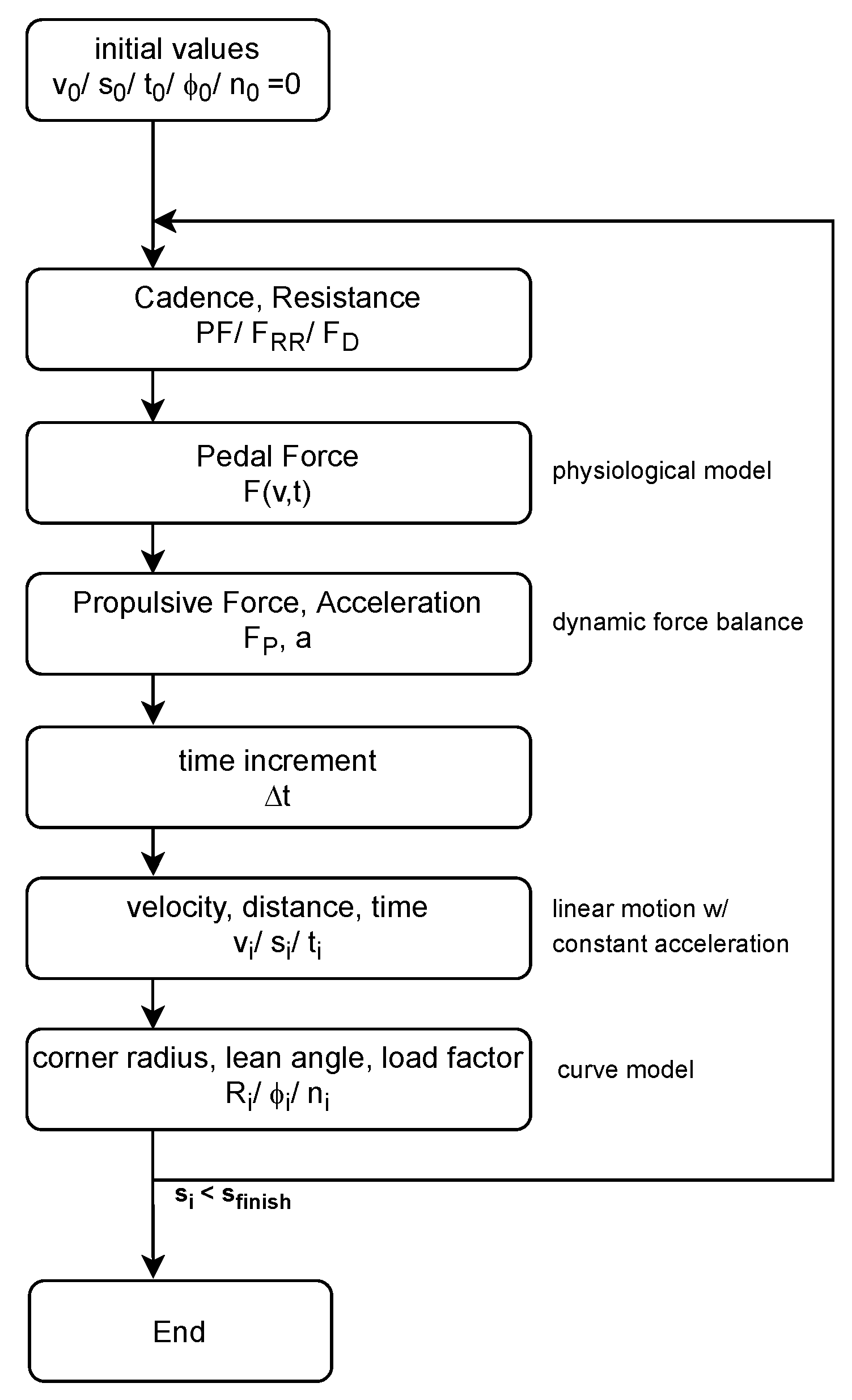
2.3. Implementation

The explicit-forward iteration of all time-dependent variables is conducted in the distance domain at equidistant points to facilitate the direct comparison of computed values to observations taken at fixed positions in the velodrome (start line, half-round, round, finish line, etc.). A suitably small increment $\Delta s$ has to be selected to account for the unsteady characteristics of all variables. Within each distance increment $\Delta s$, a non-uniform linear motion with constant acceleration is assumed.

The sequence of computational steps is outlined in Figure 1. Starting from a standstill, with initial values $t=0$, $s=0$, $v=0$, $\phi =0$, the resulting drag forces $F_D$ and $F_{RR}$ can be determined using Equations (7) and (8). The cadence $PR$ results from Equation (10). With these status variables known, the pedal force applied by the athlete is returned from the physiological model and the propulsive force at this position is estimated using Equation (16). The momentary acceleration of the system can now be calculated from the force balance in Equation (6). The time increment $\Delta t$ elapsed for moving one increment is computed by solving the differential equation of motion for the time interval t, taking into account that due to the lean angle, the centre of gravity travels a distance shorter than $\Delta s$:

$$\Delta t_{1,2}=-\frac{v}{a}\pm \sqrt{\frac{v^2}{a^2}+\frac{2\Delta s·(1-sin\phi /H)}{a}}$$

(17)

The result of the square root is positive for $a>0$, negative for $a<0$ and the case $a=0$, which is numerically most unlikely to appear, has to be excluded. Now, the initial velocity for the next distance increment can be calculated:

$$v_1=v_0+a_0·\Delta t_0$$

(18)

The absolute position of the system relative to the start and the total run-time until this position is reached results from a summation of the respective increments:

$$s=\sum \Delta s;t=\sum \Delta t$$

(19)

In this contribution, a generic track 250 m in length with circular corners of radius $R=25$ m shall be assumed. This results in a 46.46 m straight, followed by a 78.54 m long curve, with a period of 125 m. With the absolute distance known, the position $s^{*}$ within half a lap can be computed:

$$s^{*}=mod\left(\frac{d}{125\mathrm{m}}\right)$$

(20)

From $s^{*}$, the local corner radius can be determined, and the corresponding lean angle computed using Equation (11), assuming that the transition between cycling upright in the straights and inclined in the curves or vice versa occurs in a linear fashion over a distance of ca. 20 m centred around the geometric origin of the bend. Thus, the lean angle is multiplied with a form function that is defined to be zero in the straights, “1” in the bends and a linear function of s during the transition from one to the other. From this adjusted lean angle, the local load factor from Equation (12) and all derivatives thereof can be calculated.

Usually, at the start, the athlete accelerates the bike in a standing position (STAND) for the initial 140 to 170 m. This affects the aerodynamic characteristics, as well as the physiological capabilities. To account for this, a different set of parameters is used for $c_D·A$, A, $\tau$ and c for this phase. The iteration cycle is repeated until the system reaches the desired finish position.

2.4. Determination of Model Parameters

2.4.1. Track Cycling Time Trials

Six elite track cycling sprinters (19.5 ± 0.76 years, 183.50 ± 10.08 cm, 83.6 ± 13.91 kg) performed two 500 to 1000 m all-out time-trials (length specific to the athlete’s competitive event) from a standing start on an official cycling track, each with substantially different gear ratios (Frankfurt/Oder, Germany).

The athletes were requested to refrain from consuming alcohol and from intense training during the 24 h period prior to the experimental session and asked to maintain their normal drinking and eating habits. They provided written informed consent to participate in this study, which was approved by the institute’s ethical committee and performed in accordance with the Declaration of Helsinki.

2.4.2. Exercise Protocol

Before the first run, the athletes with their clothes and bikes were weighed to determine the mass of the rider-bike system. The warm-up prior to the tests consisted of 15 min of low-intensity cycling (1–1.5 W per kg bodyweight), followed by three short maximal sprints on the cycling track. The athletes rested passively for 10 min between warm-up and testing.

All athletes first performed two 6 s sets of maximal-cadence low-resistance cycling on a free-standing roller (motoric sprint) and two 6 s maximal sprints in a seated position on the track to generate additional data points in the high-frequency cadence range for a valid determination of the $F/v$ profiles. These points were added to the fatigue-free pedal revolutions from the acceleration phase of the time trials [32].

The athletes then completed two 500 to 1000 m all-out sprints from a standing start with two different gear ratios. In the first run, athletes were asked to choose their preferred gear. In the second run, a much larger gear was selected. The sprints were separated by at least 20 min of low-intensity cycling (1–1.5 W per kg bodyweight) for active recovery and 20 min passive recovery. The next test began when comparable levels of blood lactate were observed.

Throughout the testing, pedal force and crank velocity were monitored continuously with a special power meter. The system supplied by the Institute for Research and Development of Sports Equipment (FES) in Berlin captures the tangential force on the crank arm with a sampling frequency of 200 Hz. This system allows for the observation of sport-specific movements and the creation of sport-specific force-velocity and power-velocity profiles [33]. From this high-resolution power-meter data, the mean tangential force $F_T$ at both pedals, averaged per one revolution, as well as the corresponding mean pedal rate $PR$, was derived.

The air density was measured prior to each run with a commercial weather meter (KESTREL 5200, Kestrel AU) located close to the cycling track. Before and every tenth minute after each sprint, 20 µL capillary blood was collected from the hyperaemic ear lobe for haemolysis and enzymatic-amperometric determination of lactate (Biosen, Eppendorf/Germany).

2.4.3. Data Analysis

In the 500 m and 1000 m-time trials, athletes usually use a standing position in the initial phase (acceleration phase) and a seated position at high speed [2].

To establish the fatigue-free $F/v$ profile in a seated position, the first 3 or 4 cycles from the seated maximal sprint and, as proposed in [32], 1 or 2 cycles at pedal rates above 160 rpm derived from the motoric test were taken. To reproduce the performance potential of the athlete in a standing position on the bike, the $F/v$ profile was adjusted for the first 3 or 4 pedal revolutions of the acceleration phase during the standing start of each run. The profile parameters were determined by linear regression analysis, and the calculated slope was used for further analysis.

The model parameters for Equation (5) were determined by non-linear regression separately for the first phase of the race, where the athlete accelerates while standing (STAND), and for the second phase with the athlete adopting a seated position until the end of the race (SIT). A sudden systematic drop in power output in the raw data separated the two phases.

A time delay $TD$ was used to account for any delays in the onset of fatigue. To implement this delay in our model, the coefficient $F_{max}\left(t\right)$ is estimated based on the average value of the pedal force $F_T$ for time t within [0; $TD$].

The parameters derived from an athlete’s first sprint were applied to the raw biomechanical data of the following sprint. If the model quality matched the R${}^2$ of the first run, the parameters were kept constant; otherwise, the model parameters were adjusted to improve the fit.

2.4.4. Statistics

Linear regression analysis was used to study the relationship between data. The absolute value of the difference between the measured and modelled data was used to determine the bias of the measurements. Paired t-tests were employed to investigate for any difference within the data. Cohen’s d (small = 0.2; medium = 0.5; large = 0.8) was employed as a measure of effect size, with statistical significance being set at an alpha level of <0.05. All mathematical analysis and statistical tests were processed using IBM SPSS statistics version 24 Software for Windows (SPSS Inc., Chicago, IL, USA) and Office Excel 2016 (Microsoft Corporation, Redmond, WA, USA). The quality of the regression analyses was examined by calculating the coefficient of determination R${}^2$.

3. Results

Mean pedal force and the pedalling rate with corresponding power output for one athlete during both 750 m-time trials is illustrated in Figure 2. The gear ratio of the first run ($i=3.6$) corresponds to a distance of 7.56 m per pedal revolution. Here, the mean power output was 651 W at a mean cadence of 117 rpm. In the second run, a higher gear ratio $i=4.14$, resulting in the development of 8.7 m was chosen. In the second race, the mean power was 691 W at a mean cadence of 104 rpm.

In Figure 3, the maximum pedal force $F_{max}$ attained at $PR=0$ was calculated from the data measured in the first run and the physiological model fitted, returning high to excellent agreement. The physiological model parameters were then used to approximate the data measured in the consecutive run with different gearing, and the fit quality was assessed again. It was established that the physiological model can accurately reproduce the decline in $F_{max}$ with time and that this athlete-specific fatigue characteristic can be generalised and reused to forecast following runs, even in a different setup.

While this worked sufficiently well for five athletes, the physiological parameters had to be adjusted for athlete no. 6 to fit the data captured in the second run. Model parameters found for all six athletes in the two different phases (STAND, SIT) of the race with the associated model quality, measured by the determination coefficient R${}^2$, are detailed in

Table 1. Parameters of the physiological model with their coefficient of determination for the initial standing (STAND) and the following phase ridden in a seated position (SIT) (n = 6).

	Athlete	a	A	$\mathbf{\tau }$	c	R${}^2$
STAND	1	−6.03	1581.51	50.17	0.00	0.93
	2	−4.63	1151.82	60.40	0.00	0.85
	3	−7.42	2205.73	45.69	0.00	0.96
	4	−8.01	2190.36	56.48	0.00	0.82
	5	−6.80	1894.02	70.40	0.00	0.84
	6	−7.30	2261.81	46.02	0.00	0.94
SIT	1	−4.80	754.93	77.50	340.84	0.91
	2	−4.14	912.37	86.26	0.22	0.94
	3	−4.88	1121.83	19.90	675.15	0.95
	4	−4.40	1165.73	31.22	410.83	0.93
	5	−3.94	1107.77	28.13	414.44	0.96
	6	−5.30	1315.08	40.09	432.45	0.94

. When comparing the R${}^2$ of the different runs using a paired t-test, no statistically significant differences were found ($p>0.05$; $d<0.1$).

In the next step, the physiological model was tested for correct reproduction of the dependency between cadence $PR$ and mean pedal force $F_T$ by comparing the measured pedal forces to projected values. Figure 4 illustrates for all six athletes, each in two runs, the deviation between the modelled and the measured data, plotted against the distance travelled. With a bias of 2.05 N at a standard deviation of 14.77 N, the overall agreement was found to be satisfactory.

Applying the physical model to the pedal force returned by the physiological model as an input, the expected instantaneous velocity of the system and the mechanical power required by the athlete can be computed. In Figure 5, the modelled velocity at the wheels is compared to the measurements, and a very good agreement was observed. A similar comparison is displayed in Figure 6 for the mechanical power, where both quantities are highly correlated despite the data returned from the power meter showing significant fluctuations. A linear regression analysis was employed to the modelled and measured velocity and power output, respectively. A high degree of agreement was returned for both quantities.

Table 2. Correlation between the modelled and measured data of cycling velocity $v_w$ and power output with the corresponding coefficient of determination R${}^2$ (n = 6).

		First Run		Second Run
	Athlete	k	R${}^2$	k	R${}^2$
velocity $v_w$	1	1.002	0.997	1.009	0.996
	2	1.003	0.997	1.002	0.997
	3	1.007	0.993	1.005	0.998
	4	1.003	0.995	0.998	0.998
	5	1.005	0.999	1.003	0.995
	6	1.001	0.999	1.004	0.995
power output	1	0.969	0.959	0.988	0.975
	2	0.973	0.958	0.992	0.969
	3	0.982	0.976	1.002	0.998
	4	0.994	0.968	0.973	0.979
	5	1.018	0.936	0.989	0.968
	6	0.965	0.952	0.971	0.941

tabulates the R${}^2$ found in the two runs and the proportionality factor k between the modelled and measured data.

Keeping the model parameters constant for multiple runs with different setups, our combined physiological and physical model predicted the actual cycling velocity and power output with unaltered accuracy. No statistically significant differences in model quality between different runs could be observed. Figure 7 demonstrates an example for the wheel’s velocity of the same athlete as in Figure 5, captured in the second run with 15% higher gearing, and the corresponding results of the linear regression analysis.

Finally, Figure 8 illustrates the dispersion of the modelled data points for velocity related to the distance travelled across all data sets from six athletes. It becomes apparent that larger deviations between modelled and measured data appear primarily in the standing phase of the runs.

4. Discussion

We experimentally demonstrated, in test runs with six athletes, that using our combined physio-physical model, time trial track cycling performed in an all-out fashion can be modelled, and the results can be predicted with reasonable precision. This enables the evaluation of each individual factor’s contribution to the overall performance.

A generic rider was created as proposed in [24], with its physiological parameters derived from the arithmetic mean of the respective parameters found on our six individual athletes. Figure 9 depicts the sensitivity of the run-time for a change in the system’s mass for distances of 250 to 1000 m. For each distance, a monotonous linear correlation was observed. The slope of these curves decreases with the increasing length of the run, indicating that the effect of a change in the system’s mass is more prominent in short-distance races. This is plausible, as an increase in mass is particularly detrimental during the acceleration phase. Once accelerated, mass only affects the rolling resistance, which is orders of magnitude smaller than the inertia force.

In Figure 10, the effect of a change in aerodynamic drag area on run-time is shown for four different distances. This result is particularly useful as it helps to translate an improvement found by wind-tunnel measurements into run-time savings on the track. In contrast to the effect of a change in mass, the importance of a change in aerodynamic drag increases with increasing run distance, as is apparent by the slope of the curves becoming steeper. As aerodynamic resistance is proportional to v${}^2$, its impact increases at higher speeds and accumulates over time.

Perhaps the most relevant setup parameter is the gear-ratio, physically coupling power available and power required. It cannot be changed during the effort but has to be chosen carefully in advance. A relatively low gear ratio will augment the acceleration of the system at the expense of premature fatigue of the cyclist, while too high a gear ratio will keep the athlete from reaching top speed in a reasonable time. Our model can be used to create individual gear ratio profiles and determine an athlete’s optimal gear for different race distances.

Figure 11 exhibits the expected change in run-time of the generic athlete, normalised to the minimum run-time found, for four race distances at different developments, i.e., the distance travelled per one crank revolution. A distinct optimum development, resulting in the shortest possible run-time under given circumstances and training level, can be observed at 0%. This optimum is shifted towards higher gearing with increasing race distance. This observation is supported by practical experience: short-distance events are dominated by start performance, which is improved with lower gearing, while longer distances emphasise maintaining a high speed for a prolonged time, where a higher gearing is advantageous.

Comparing the gradient of the curves left and right of the apex, it becomes evident that too high a gear ratio is less detrimental on the run-time than a gear ratio too low by the same amount. In practice, this implies that if there is uncertainty about the individual optimum, it is advisable to select a gear that is slightly too large rather than one that is slightly too small. To our knowledge, this observation is in contradiction to the recent common practice on the track.

Similar studies can be conducted with regard to the athlete’s physiological parameters. In Figure 12, the time constant $\tau$ of the generic rider, which is a measure linked to its individual resistance to fatigue, was varied. For short races, the importance of the time constant, or endurance, is much lower than for longer distances.

A congruent observation is found for the sensitivity of the run-time for changes in the residual value c, to which the pedal force drops when fatigue is “fully” developed and which, according to Monod and Scherrer’s critical power concept [34], may be related to an athlete’s aerobic power. After a 250 m run, this situation is not yet reached, but it is realised in longer efforts of up to 1000 m. Consequently, in Figure 13, the graph for 250 m shows a negligible impact, while at 1000 m, a linear correlation is present.

In Figure 14, the effect of maximum power attainable for the non-fatigued athlete on run-time is studied. It is important to note that all curves collapse on the same line, rendering this correlation independent from a distance. The gradient slightly decreases with increasing level of $P_{max}$, indicating that for every step gained in maximum power by, e.g., training, an ever-smaller benefit in run-time will be achieved. This is mainly caused by the aerodynamic drag being proportional to v${}^2$, the power required to maintain a given velocity increasing rapidly with v${}^3$. Nevertheless, changes in $P_{max}$ show nominally the largest impact on run-time.

Our physical model describing the demand side of the energy budget is based on fundamental engineering and physical principles and is similar to various models proposed by previous investigators [5,6,7,8,9,10,11,12,13].

The innovative element in our contribution is the combination of a physical model describing the instantaneous energy demand in time-trial track cycling with a description of maximal fatigue-free power output and fatigue characteristics as current maximal cadence-independent biomechanical performance. This enables the computing of (future) time-dependent power output for any setup or ambient conditions. This aspect has recently been re-identified as one of the most important topics for research in track cycling by Ferguson et al. [17].

The physiological model is reliable and reproduces the athlete’s current performance potential with reasonable accuracy, provided that the athlete performs in an all-out fashion and, in the case of multiple runs, that fatigue is controlled by an appropriate recovery protocol during the rest phase. Our results suggest that power development potentiation effects after activation can increase power output in cycling [35], while fatigue can decrease it [36,37].

The fatigue-free power output had to be slightly adjusted for the accurate reconstruction of the second run for one athlete. To avoid a misjudgement due to an unaddressed change in fatigue-free power output, the fatigue-free $F/v$ profile should be retested shortly before the start of each run.

Physical performance is also subject to daily fluctuations [38], so a regular, preferably daily adjustment of the personal model parameters would be beneficial to ensure a sufficiently good prediction quality. Expanding this idea, the physiological model parameters also offer the possibility to document and analyse individual biomechanical performance in a more generalised way on a long-term basis. A clarification of the physiological background of the model parameters should be the subject of future research.

All data sets yielded larger deviations between modelled and measured values in the STAND phase of the runs. This phenomenon occurs due to the initial crank revolutions, which differ from the systematic scheme of the following regression, were estimated using an average value. In addition, the measured raw data showed a high degree of inconsistency, particularly in this initial phase, which proved difficult to accurately implement in the model. This inconsistency is presumably due to the coordinatively demanding situation of starting out of a starting machine with maximum acceleration. As long as the athlete is capable of starting in a similar manner in subsequent runs, our model can be carefully adjusted individually, and a comparison amongst several runs and between modelled and measured data is feasible. For less capable athletes, a start where the athlete is held by hand in a sitting position may be required.

5. Conclusions

A novel approach of modelling time trial track cycling to predict sprint performance is presented. It combines a physiological model for the athlete’s instantaneous power output with a physical model that returns the transient power required for cycling. A comparison of the power output and velocity data predicted by the model with actual measurement values confirmed its validity.

Models accurately replicating a known performance using known power output–time characteristics exist. Our contribution expands this knowledge by achieving a comparable accuracy with generalised maximal power output and fatigue characteristics measured beforehand, independent of the actual run or setup. By varying the gear ratio and calculating the time-dependent power output and cycling velocity for several runs, we demonstrated experimentally that our method is capable of predicting time trial results with good accuracy.

This combined model provides a useful means to assess and optimise the performance of individual athletes on a theoretical basis. It enables users to study the isolated effect of single parameter changes, translate improvements made by training and technical optimisation into increases in performance, and optimise multiple other variables in a way that the mean velocity during the effort is maximised and run-time reduced.

In this first attempt, only factors of fundamental importance were considered. During the track tests in the velodrome, we experienced that the impact of unsteady start performance on the results of each run was especially severe, rendering any further sophistication of the physical or physiological model unnecessary for training purposes in time-trial track cycling. Instead, the method was deliberately kept as simple as possible to promote its application in practice. All input values necessary to calibrate the model can be measured in standard performance tests or derived by the analysis of training data.

References

- Craig, N.P.; Norton, K.I. Characteristics of track cycling. Sports Med. 2001, 31, 457–468. [Google Scholar] [CrossRef]
- Douglas, J.; Ross, A.; Martin, J.C. Maximal muscular power: Lessons from sprint cycling. Sports Med. Open 2021, 7, 48. [Google Scholar] [CrossRef]
- Dunst, A.K. Trends und Perspektiven im Radsport—Der Trend großer Übersetzungen und seine Konsequenz für das physiologische Anforderungsprofil im Bahnradsprint. Leistungssport 2021, 5, 34–37. [Google Scholar]
- Olds, T.S. Modelling Human Locomotion: Applications to Cycling. Sports Med. 2001, 31, 497–509. [Google Scholar] [CrossRef]
- Di Prampero, P.E.; Cortili, G.; Mognoni, P.; Saibene, F. Equation of motion of a cyclist. J. Appl. Physiol. 1979, 47, 201–206. [Google Scholar] [CrossRef]
- Olds, T.S.; Norton, K.I.; Craig, N.P. Mathematical model of cycling performance. J. Appl. Physiol. 1993, 75, 730–737. [Google Scholar] [CrossRef] [PubMed]
- Olds, T.S.; Norton, K.I.; Lowe, E.L.; Olive, S.; Ly, S. Modelling road-cycling performance. J. Appl. Physiol. 1995, 78, 1596–1611. [Google Scholar] [CrossRef] [PubMed]
- Fitton, B.; Symons, D. A mathematical model for simulating cycling: Applied to track cycling. Sports Eng. 2018, 21, 409–418. [Google Scholar] [CrossRef]
- Davies, C.T. Effect of air resistance on the metabolic cost and performance of cycling. Eur. J. Appl. Physiol. Occup. Physiol. 1980, 45, 245–249. [Google Scholar] [CrossRef]
- Kyle, C.R. The mechanics and aerodynamics of cycling. Med. Sci. Asp. Cycl. 1988, 235, 251. [Google Scholar]
- Lukes, R.; Carré, M.; Haake, S. Track Cycling: An Analytical Model. In The Engineering of Sport; Moritz, E.F., Haake, S., Eds.; Springer: Berlin/Heidelberg, Germany, 2006; pp. 115–120. [Google Scholar]
- Martin, J.; Gardner, A.S.; Barras, M.; Martin, D.T. Modelling Sprint Cycling Using Field-Derived Parameters and Forward Integration. Med. Sci. Sports Exerc. 2006, 38, 592–597. [Google Scholar] [CrossRef] [PubMed] [Green Version]
- Underwood, L.; Jeremy, M. Mathematical model of track cycling: The individual pursuit. Procedia Eng. 2010, 2, 3217–3222. [Google Scholar] [CrossRef] [Green Version]
- Flyger, N.; Froncioni, A.M.; Martin, D.T.; Billaut, F.; Aughey, R.J.; James, C.; Martin, J.C. Modelling track cycling standing start performance: Combining energy supply and energy demand. In Proceedings of the ISBS Conference Proceedings Archive 31th International Conference on Biomechanics in Sports, Taipei, Taiwan, 7–11 July 2013. [Google Scholar]
- Martin, J.C.; Milliken, D.L.; Cobb, J.E.; McFadden, K.L.; Coggan, A.R. Validation of a Mathematical Model for Road Cycling Power. J. Appl. Biomech. 1998, 14, 276–291. [Google Scholar] [CrossRef] [PubMed] [Green Version]
- Quod, M.J.; Martin, D.T.; Martin, J.C.; Laursen, P.B. The power profile predicts road cycling MMP. Int. J. Sports Med. 2010, 31, 397–401. [Google Scholar] [CrossRef] [PubMed]
- Ferguson, H.A.; Harnsih, C.; Chase, J.G. Using Field Based Data to Model Sprint Track Cycling Performance. Sports Med. Open 2021, 7, 20. [Google Scholar] [CrossRef]
- Gardner, A.S.; Martin, D.T.; Jenkins, D.G.; Dyer, I.; Achten, J.; Barras, M.; Martin, J.C. Velocity-Specific Fatigue: Quantifying fatigue during variable velocity cycling. Med. Sci. Sports Exerc. 2009, 41, 904–911. [Google Scholar] [CrossRef]
- De Koning, J.J.; Bobbert, M.F.; Foster, C. Determination of optimal pacing strategy in track cycling with an energy flow model. J. Sci. Med. Sport 1999, 2, 266–277. [Google Scholar] [CrossRef]
- McCartney, N.; Heigenhauser, G.J.; Jones, N.L. Power output and fatigue of human muscle in maximal cycling exercise. J. Appl. Physiol. 1983, 55, 218–224. [Google Scholar] [CrossRef]
- Seow, C.Y. Hill’s equation of msucle performance and its hidden insight on molecular mechanisms. J. Gen. Physiol. 2013, 142, 561–573. [Google Scholar] [CrossRef] [Green Version]
- Dorel, S.; Hautier, C.A.; Rambaud, O.; Rouffet, D.; Van Praagh, E.L. Torque and power–velocity relationships in cycling: Relevance to track sprint performance in world-class cyclists. Int. J. Sports Med. 2005, 26, 739–746. [Google Scholar] [CrossRef]
- Gardner, A.S.; Martin, J.C.; Martin, D.T.; Barras, M.; Jenkins, D.G. Maximal torque- and power-pedaling rate relationships for elite sprint cyclists in laboratory and field tests. Eur. J. Appl. Physiol. 2007, 101, 287–292. [Google Scholar] [CrossRef] [PubMed]
- Martin, J.C.; Wagner, B.M.; Coyle, E.F. Inertial-load method determines maximal cycling power in a single exercise bout. Med. Sci. Sports Exerc. 1997, 29, 1505–1512. [Google Scholar] [CrossRef]
- Dorel, S. Maximal force-velocity and power-velocity characteristics in cycling: Assessment and relevance. In Biomechanics of Training and Testing; Morin, J.B., Samozino, P., Eds.; Springer: Cham, Switzerland, 2018; pp. 7–31. [Google Scholar]
- De Ruiter, C.; Jones, D.; Sargeant, A.; De Haan, A. The measurement of force/velocity relationships of fresh and fatigued human adductor pollicis muscle. Eur. J. Appl. Physiol. 1999, 80, 386–393. [Google Scholar] [CrossRef] [PubMed]
- De Ruiter, C.J.; Didden, W.J.M.; Jones, D.A.; De Haan, A. The force-velocity relationship of human adductor pollicis muscle during stretch and the effects of fatigue. J. Physiol. 2000, 526, 671–681. [Google Scholar] [CrossRef]
- Sargeant, A.J. Human power output and muscle fatigue. Int. J. Sports Med. 1994, 15, 116–121. [Google Scholar] [CrossRef]
- Bogdanis, G.C.; Papaspyrou, A.; Theos, A.; Maridaki, M. Influence of resistive load on power output and fatigue during intermittent sprint cycling exercise in children. Eur. J. Appl. Physiol. 2007, 101, 313–320. [Google Scholar] [CrossRef]
- Buttelli, O.; Seck, D.V.; Ewalle, H.; Jouanin, J.C.; Monod, H. Effect of fatigue on maximal velocity and maximal torque during short exhausting cycling. Eur. J. Appl. Physiol. Occup. Physiol. 1996, 73, 175–179. [Google Scholar] [CrossRef] [PubMed]
- Dunst, A.K.; Grüneberger, R.; Holmberg, H.-C. Modelling optimal cadence as a function of time during maximal sprint exercises can improve performance in elite track cyclists. J. Appl. Sci. 2021; under review. [Google Scholar]
- Dunst, A.K.; Hesse, C. Trends und Perspektiven im Radsport—Geschwindigkeitsbasiertes Training in der Praxis. Leistungssport, 2022; 1, in print. [Google Scholar]
- Dunst, A.K. Anwendung von Kraft-Geschwindigkeits-Profilen im Bahnradsport. In Kräftiger, Schneller, Ausdauernder—Entwicklung der Muskulären Leistung im Hochleistungstraining; Lehmann, F., Wenzel, U., Sandau, I., Eds.; Meyer & Meyer Verlag: Aachen, Germany, 2020; pp. 113–120. [Google Scholar]
- Monod, H.; Scherrer, J. The work capacity of a synergic muscular group. Ergonomics 1965, 8, 329–338. [Google Scholar] [CrossRef]
- Doma, K.; Leicht, A.S.; Schumann, M.; Nagata, A.; Senzaki, K.; Woods, C.E. Postactivation potentiation effect of overloaded cycling on subsequent cycling Wingate performance. J. Sports Med. Phys. Fit. 2019, 59, 217–222. [Google Scholar] [CrossRef] [PubMed]
- Mader, A.; Heck, H. Energiestoffwechselregulation, Erweiterung des theoretischen Konzepts und seiner Begründungen—Nachweis der praktischen Nützlichkeit der Simulation des Energiestoffwechsels. Brennpkt. Sportwiss. 1994, 8, 124–162. [Google Scholar]
- Morin, J.B.; Samozino, P.; Edouard, P.; Tomazin, K. Effect of fatigue on force production and force application technique during repeated sprints. J. Biomech. 2011, 44, 2719–2723. [Google Scholar] [CrossRef] [PubMed]
- Jovanovic, M.; Flanagon, E.P. From The Field–Reseached Applications of the Velocity Based Strength Training. Available online: Https://www.strengthandconditioning.org/jasc-22-2/1002-from-the-field-researched-applications-of-velocity-based-strength-training (accessed on 7 October 2019).