Figure 1.
Compatibility conditions. Example between 3 sub-bodies (sb1, sb2, sb3).
Figure 1.
Compatibility conditions. Example between 3 sub-bodies (sb1, sb2, sb3).
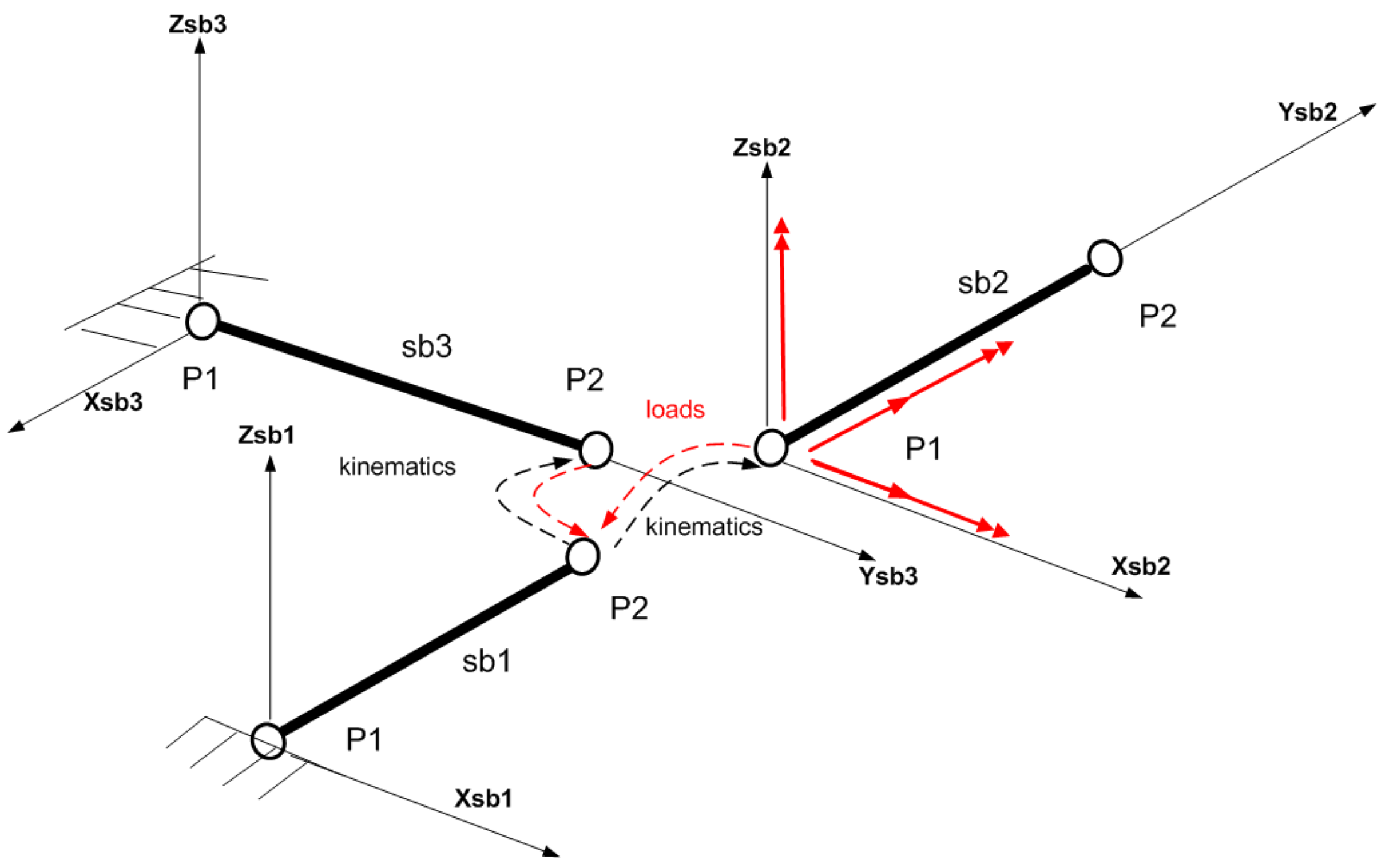
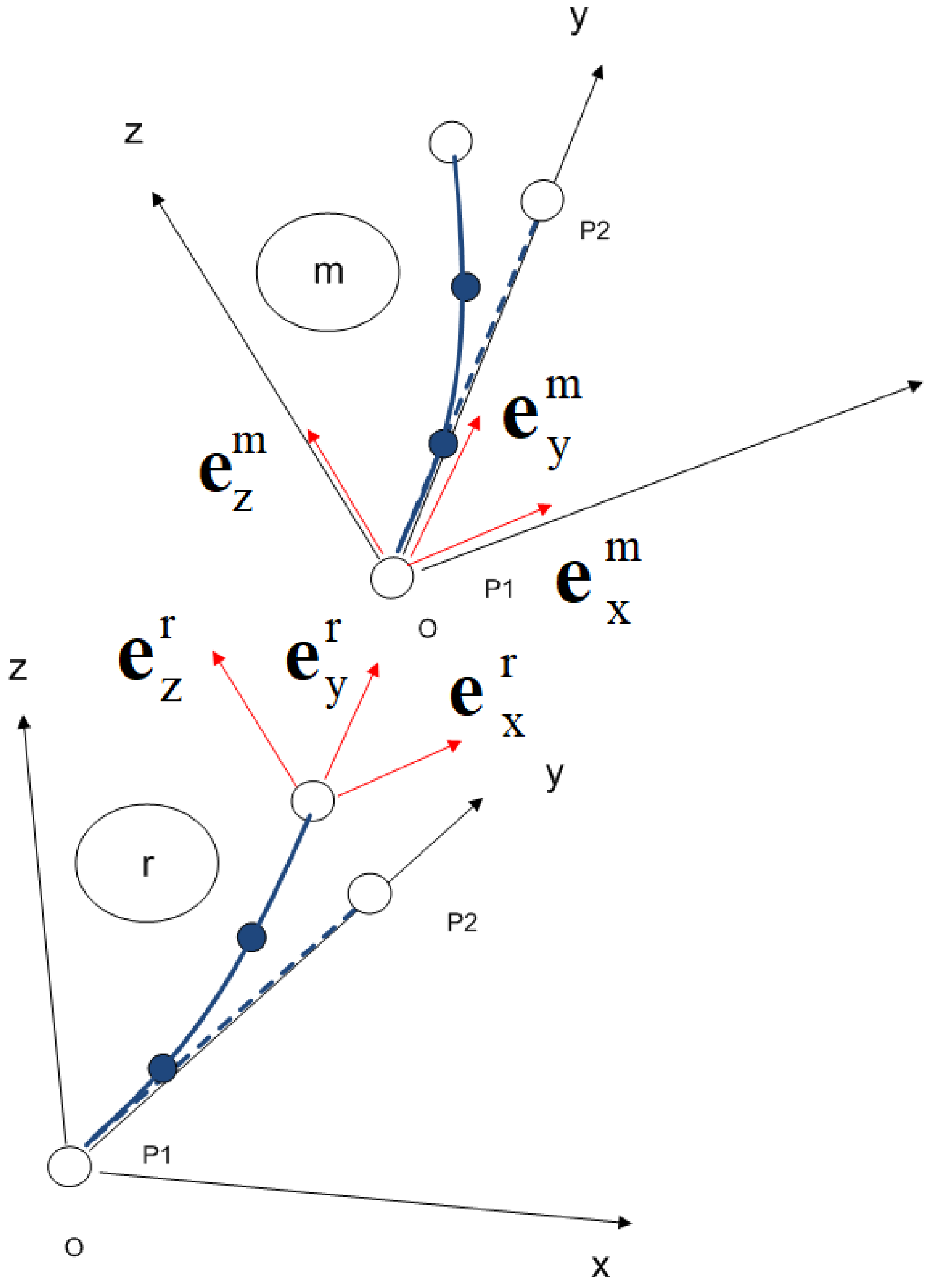
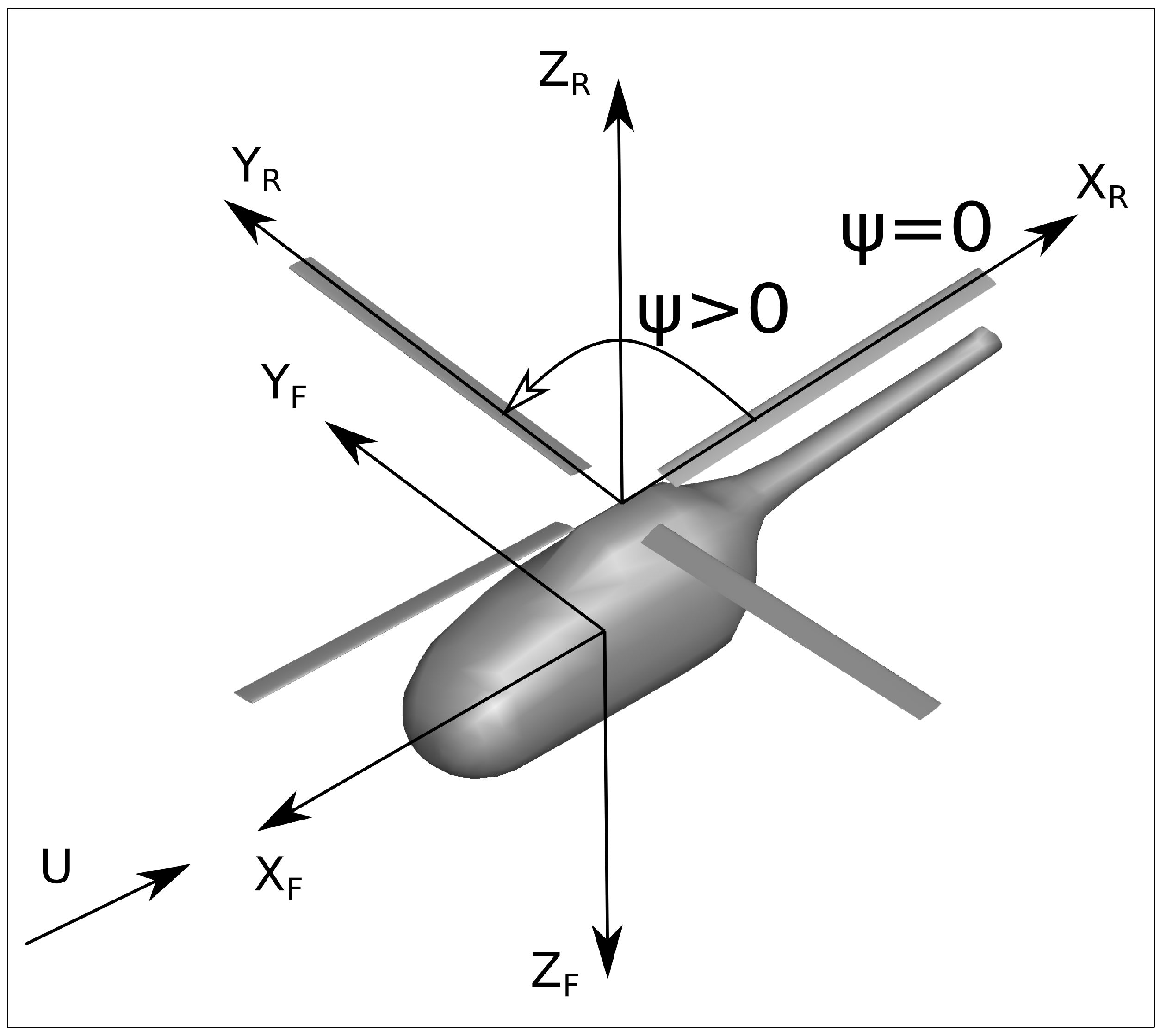
Figure 2.
Local bases vectors of interconnection points.
Figure 2.
Local bases vectors of interconnection points.
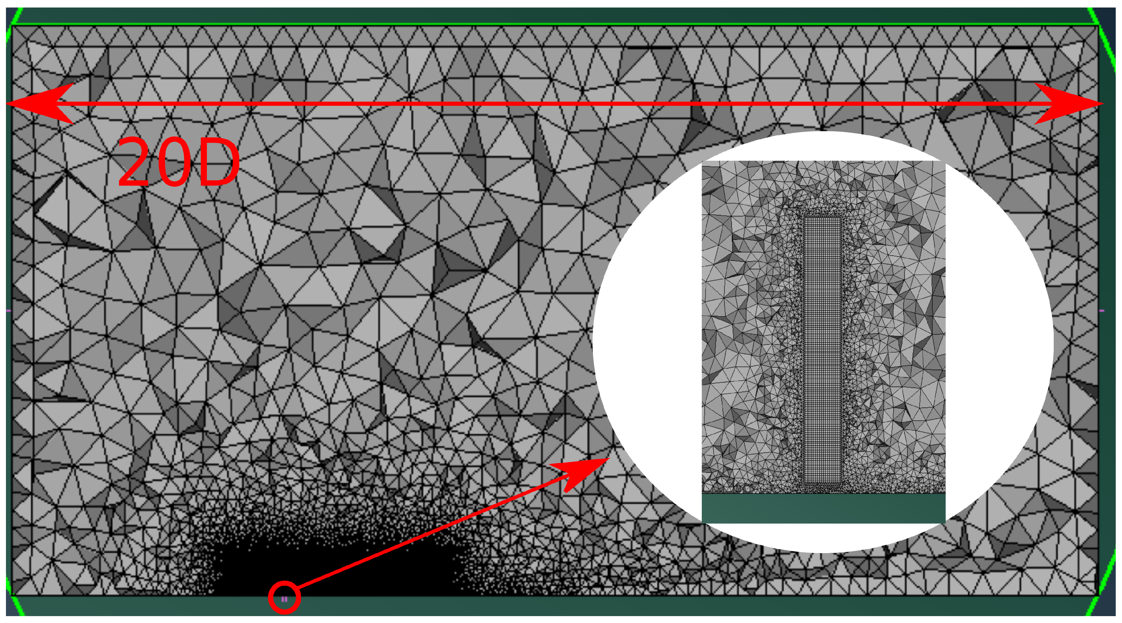
Figure 3.
Periodic grid. Lateral view.
Figure 3.
Periodic grid. Lateral view.
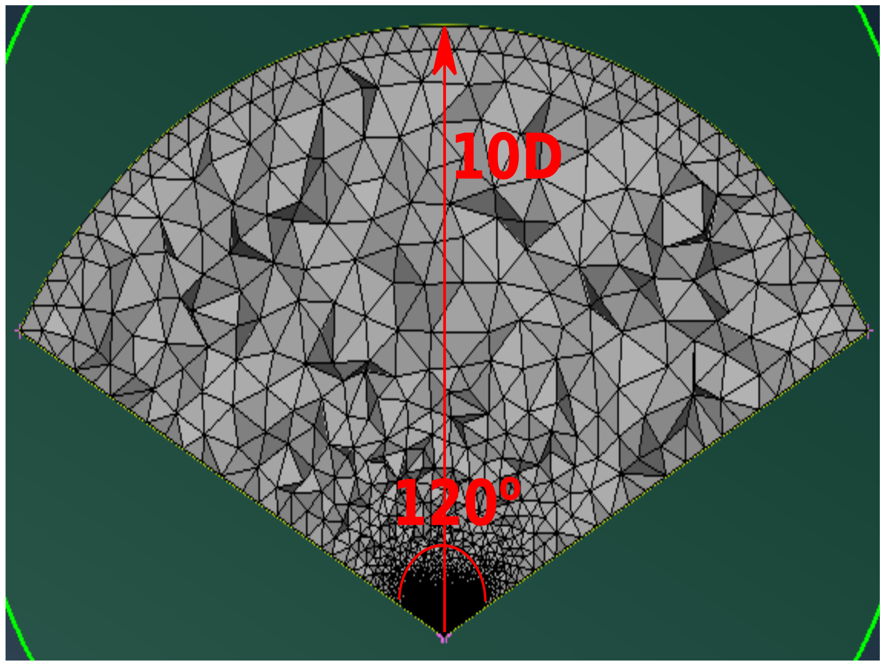
Figure 4.
Periodic grid. Axial view.
Figure 4.
Periodic grid. Axial view.
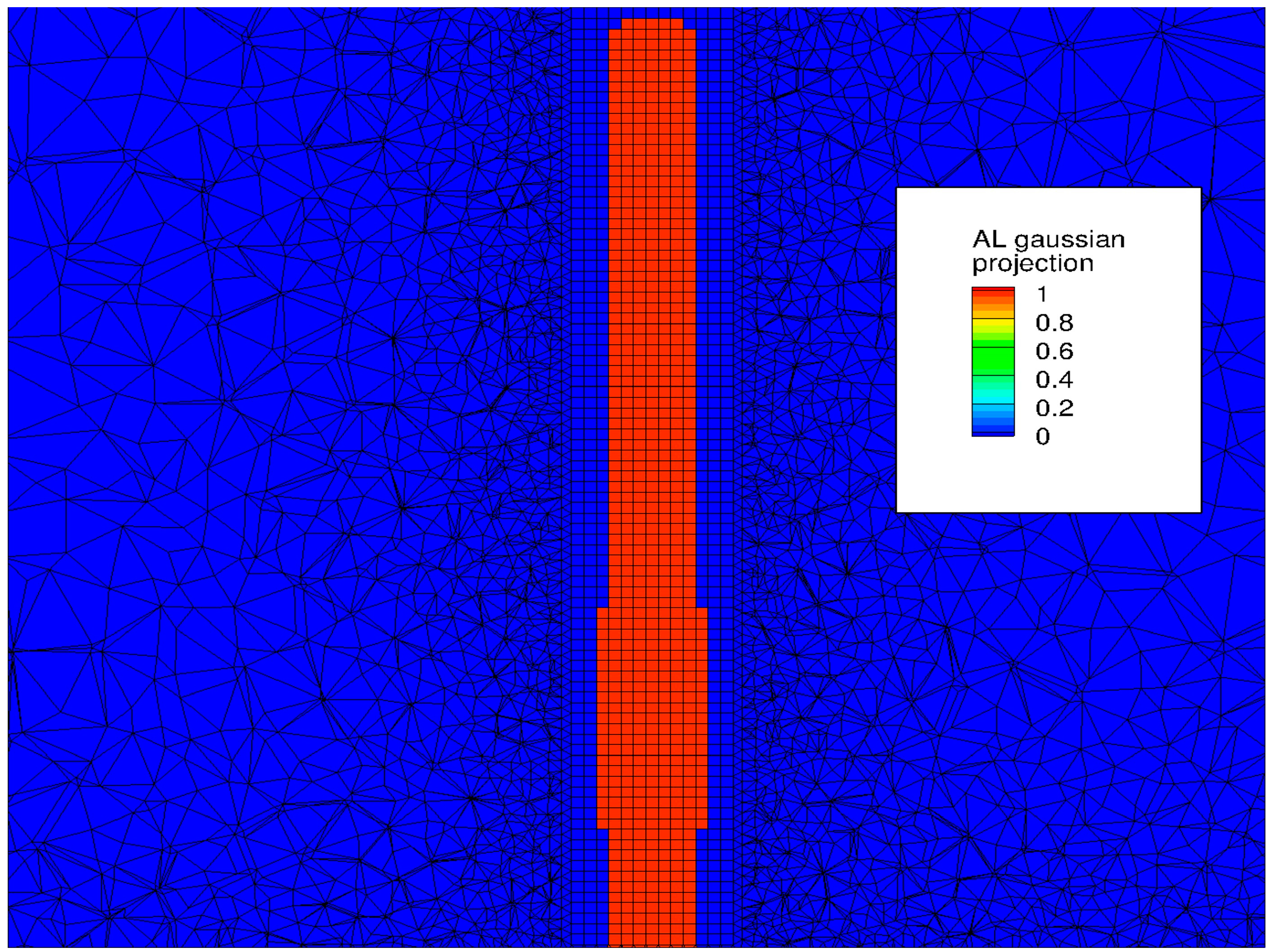
Figure 5.
Periodic grid. Gaussian projection of aerodynamic forces.
Figure 5.
Periodic grid. Gaussian projection of aerodynamic forces.
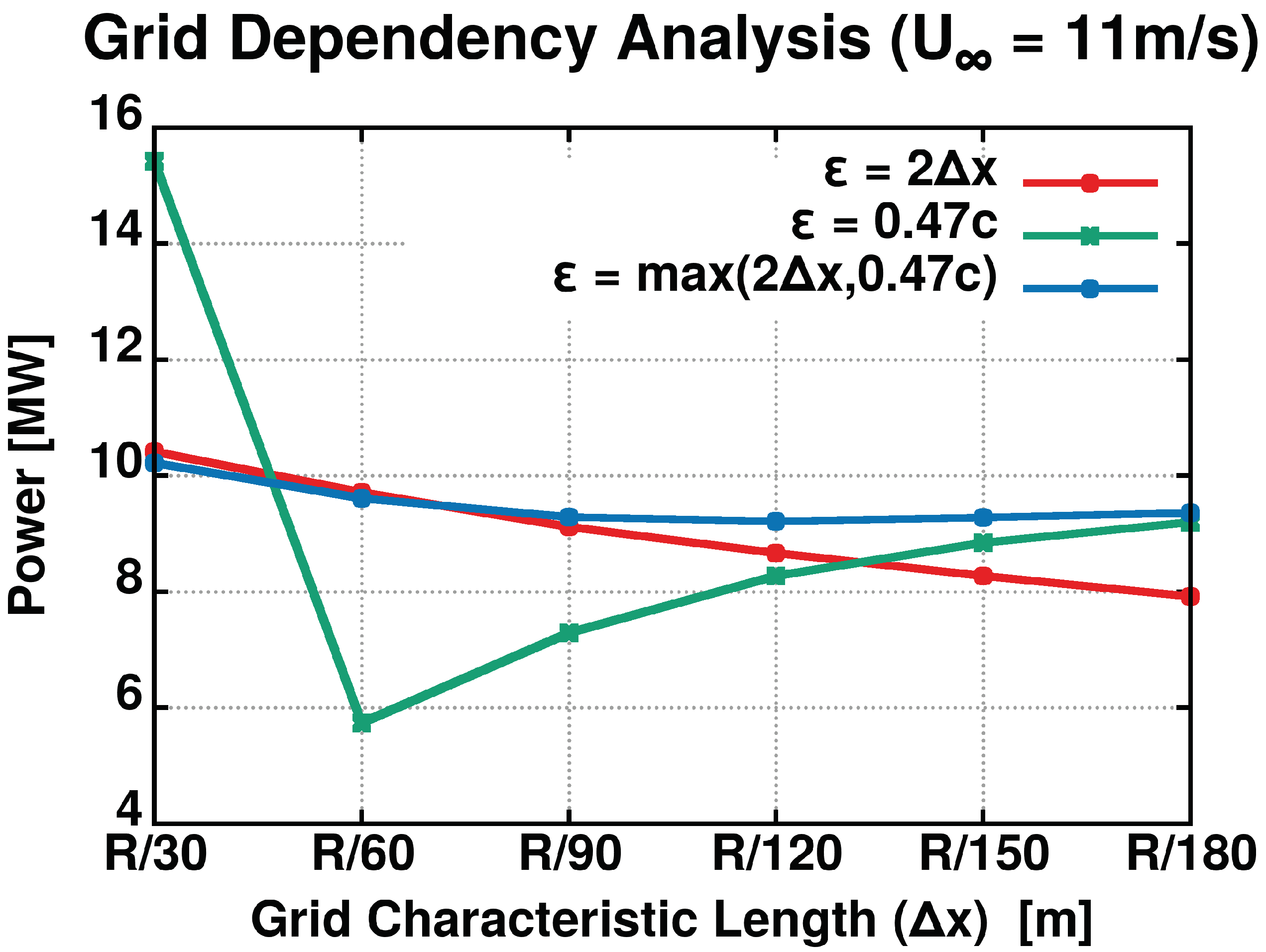
Figure 6.
Grid dependency analysis. Power [MW] vs grid characteristic length [m].
Figure 6.
Grid dependency analysis. Power [MW] vs grid characteristic length [m].
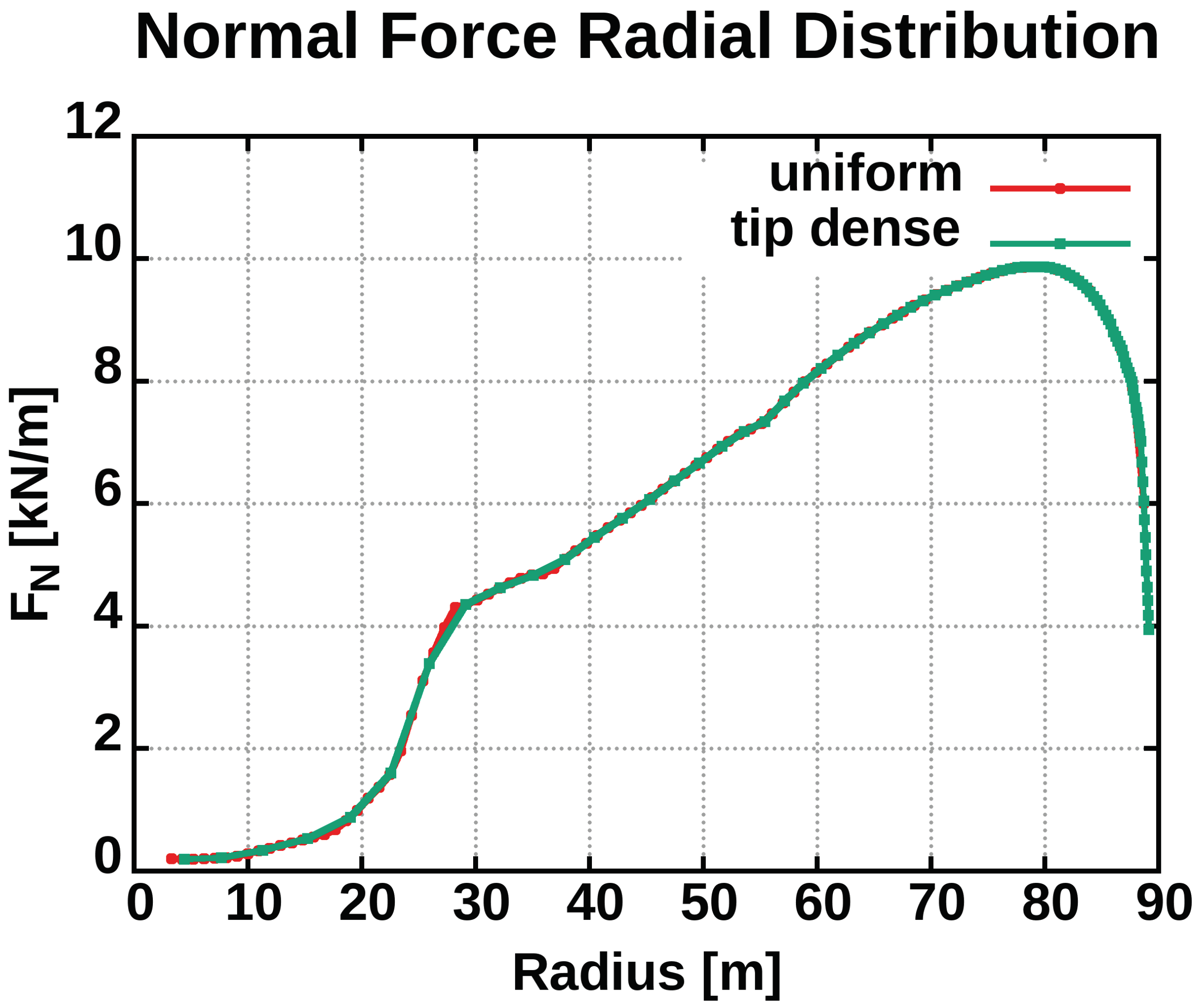
Figure 7.
Normal force radial distribution. Comparison of uniform and tip dense distribution of strips.
Figure 7.
Normal force radial distribution. Comparison of uniform and tip dense distribution of strips.
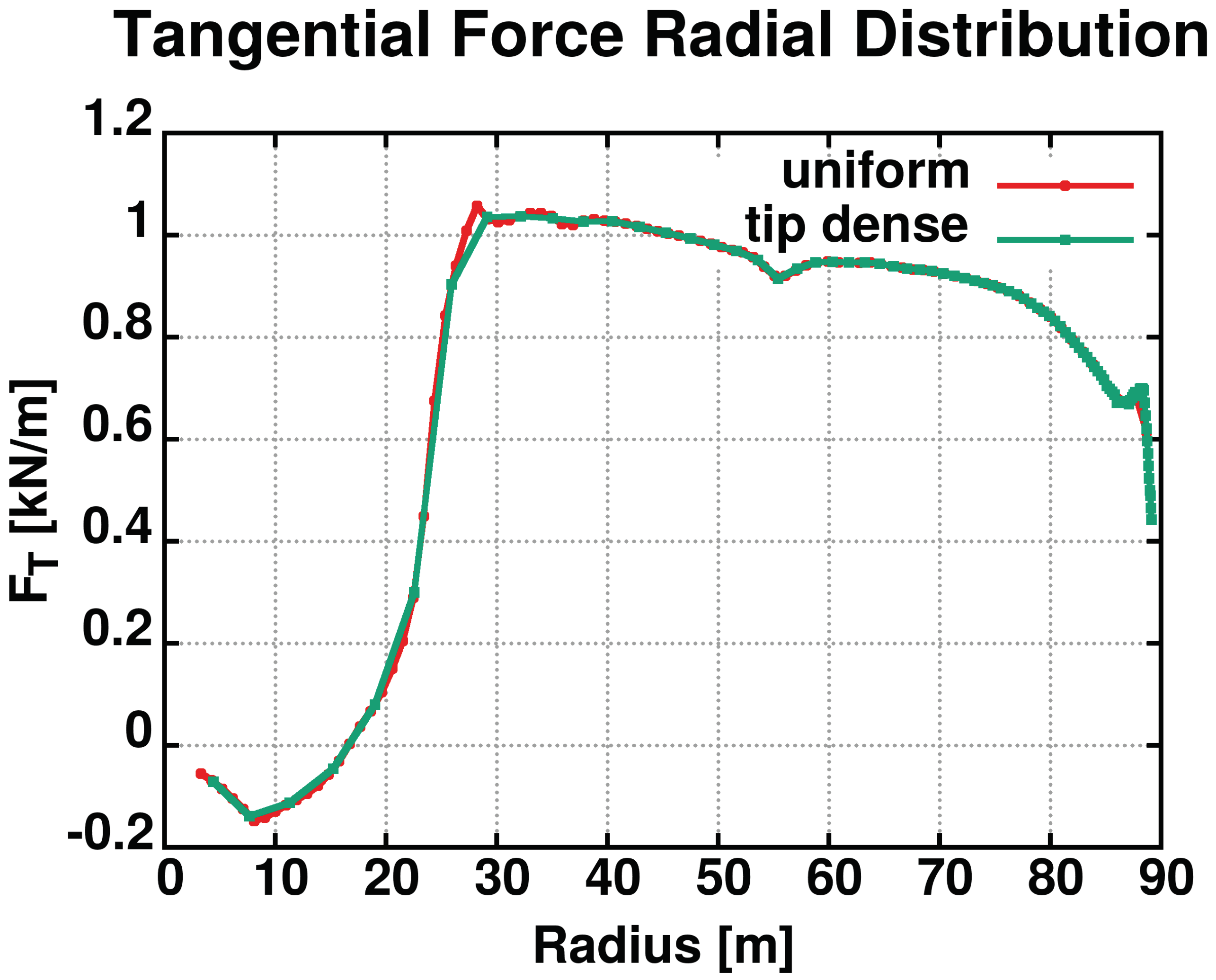
Figure 8.
Tangential force radial distribution. Comparison of uniform and tip dense distribution of strips.
Figure 8.
Tangential force radial distribution. Comparison of uniform and tip dense distribution of strips.
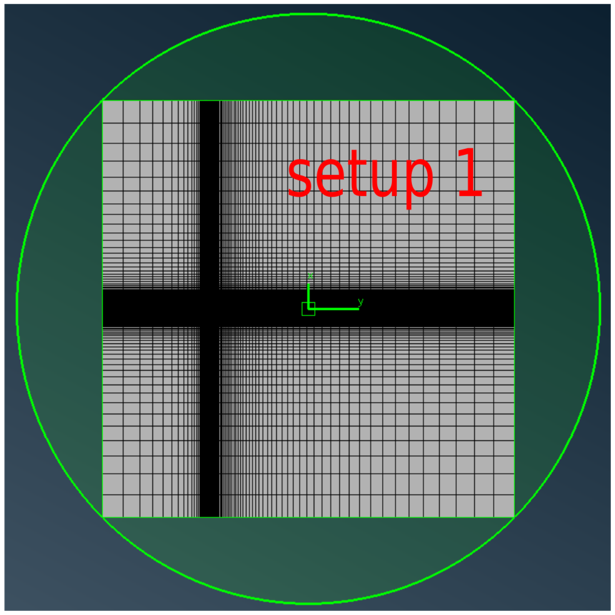
Figure 9.
Wind turbine fully structured grid setup.
Figure 9.
Wind turbine fully structured grid setup.
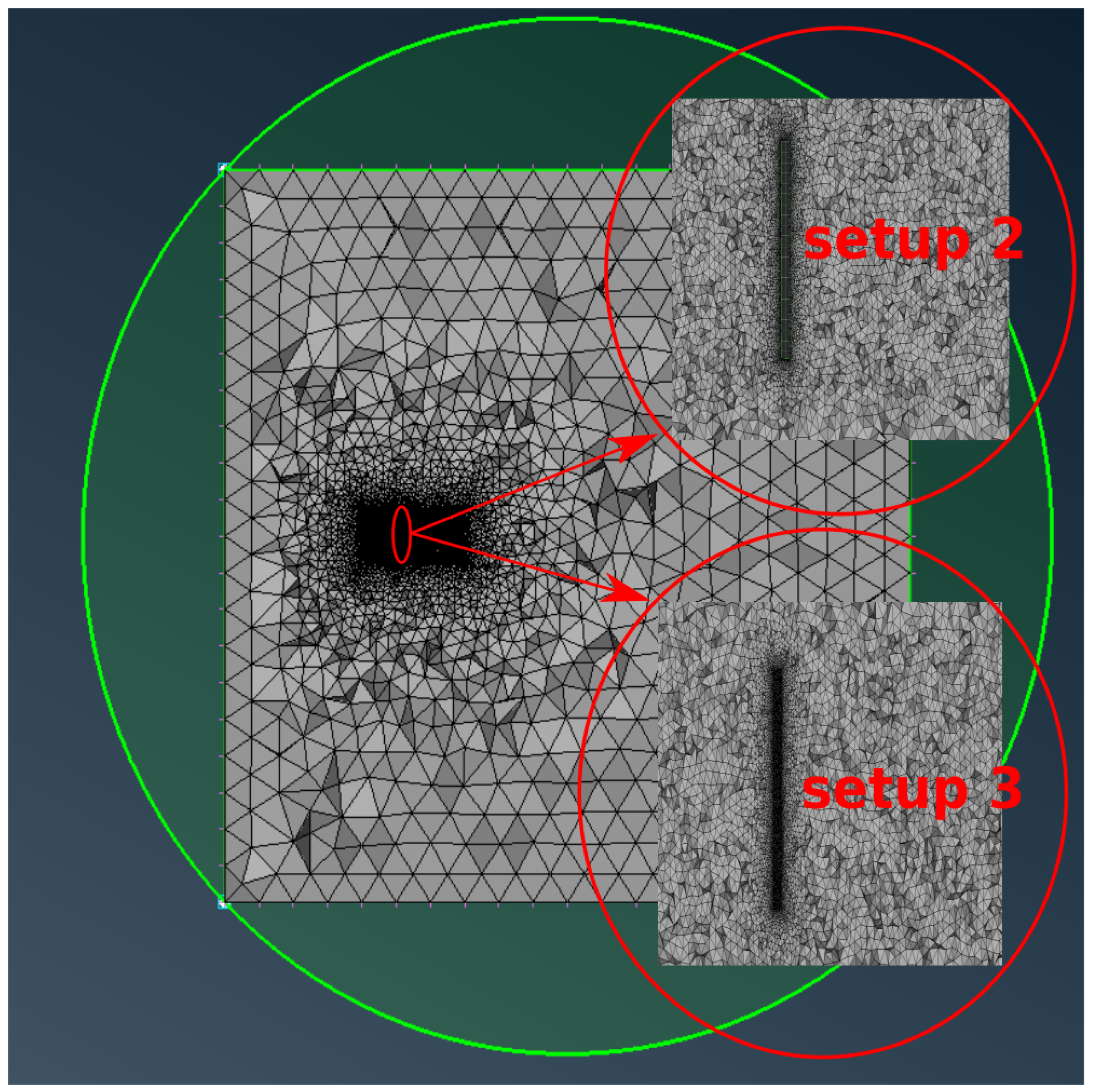
Figure 10.
Wind turbine unstructured grid setup.
Figure 10.
Wind turbine unstructured grid setup.
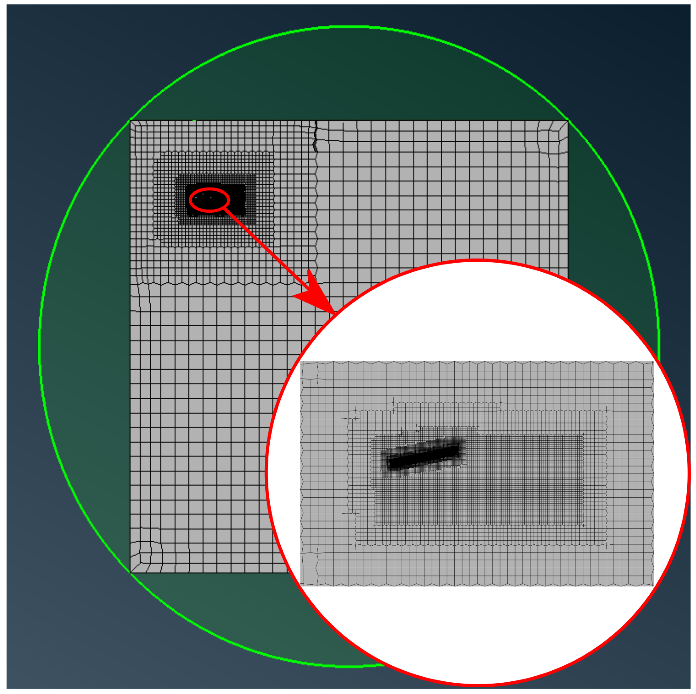
Figure 11.
Wind turbine hexa grid setup.
Figure 11.
Wind turbine hexa grid setup.
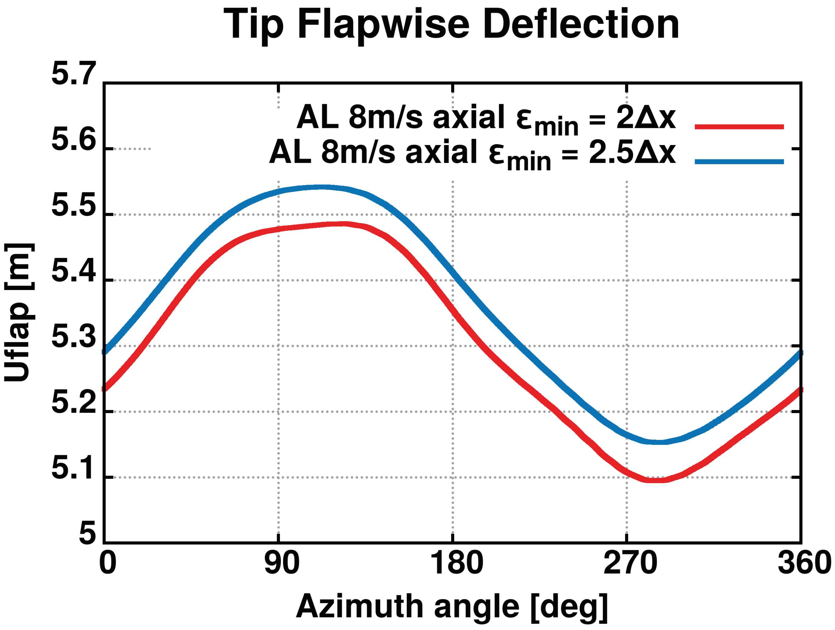
Figure 12.
Minimum value of investigation. Flapwise deflection in axial uniform free-stream flow at 8 m/s.
Figure 12.
Minimum value of investigation. Flapwise deflection in axial uniform free-stream flow at 8 m/s.
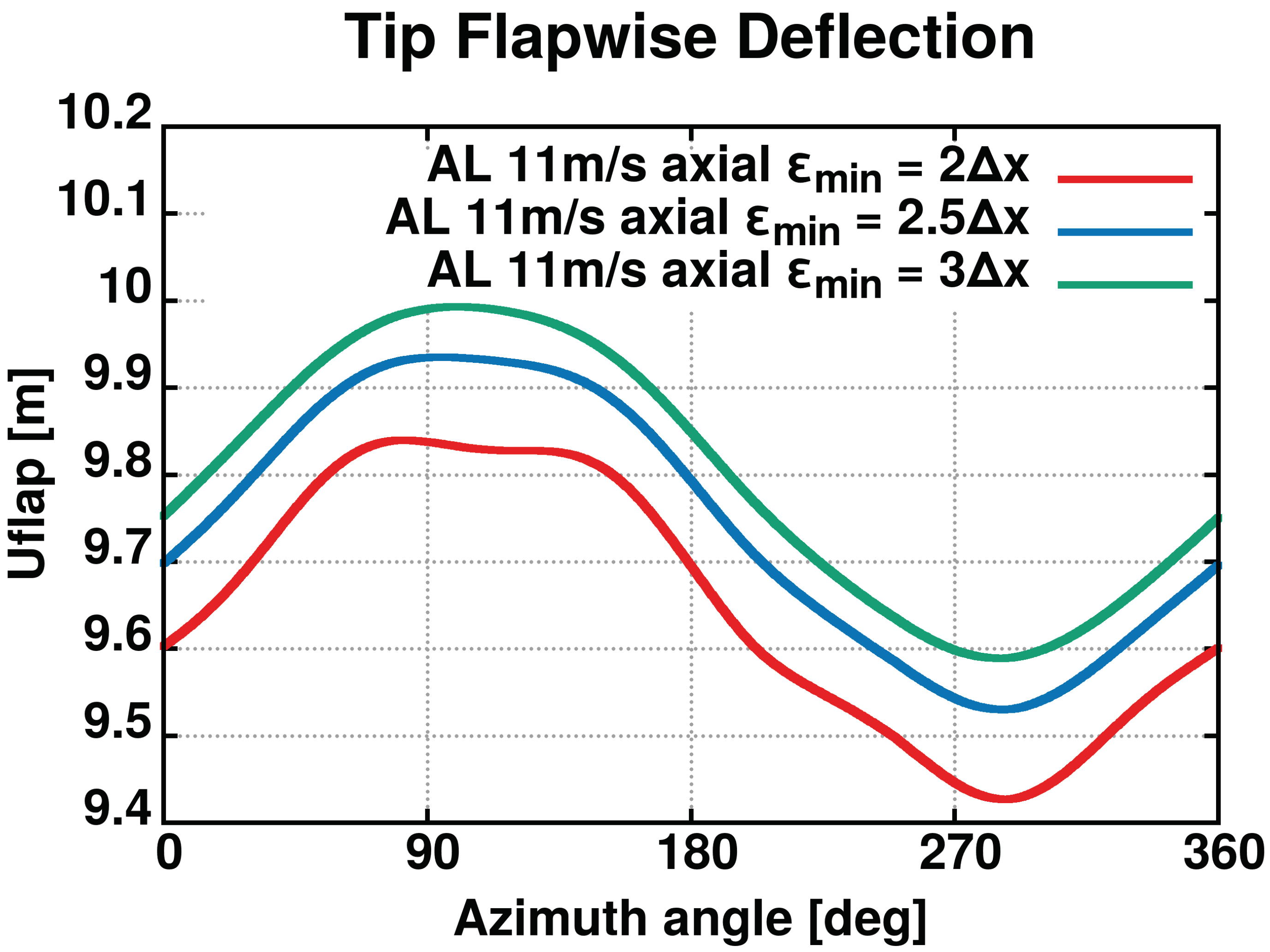
Figure 13.
Minimum value of investigation. Flapwise deflection in axial uniform free-stream flow at 11 m/s.
Figure 13.
Minimum value of investigation. Flapwise deflection in axial uniform free-stream flow at 11 m/s.
Figure 14.
MR hexa grid setup.
Figure 14.
MR hexa grid setup.
Figure 15.
Mode shape of 1st flapwise mode.
Figure 15.
Mode shape of 1st flapwise mode.
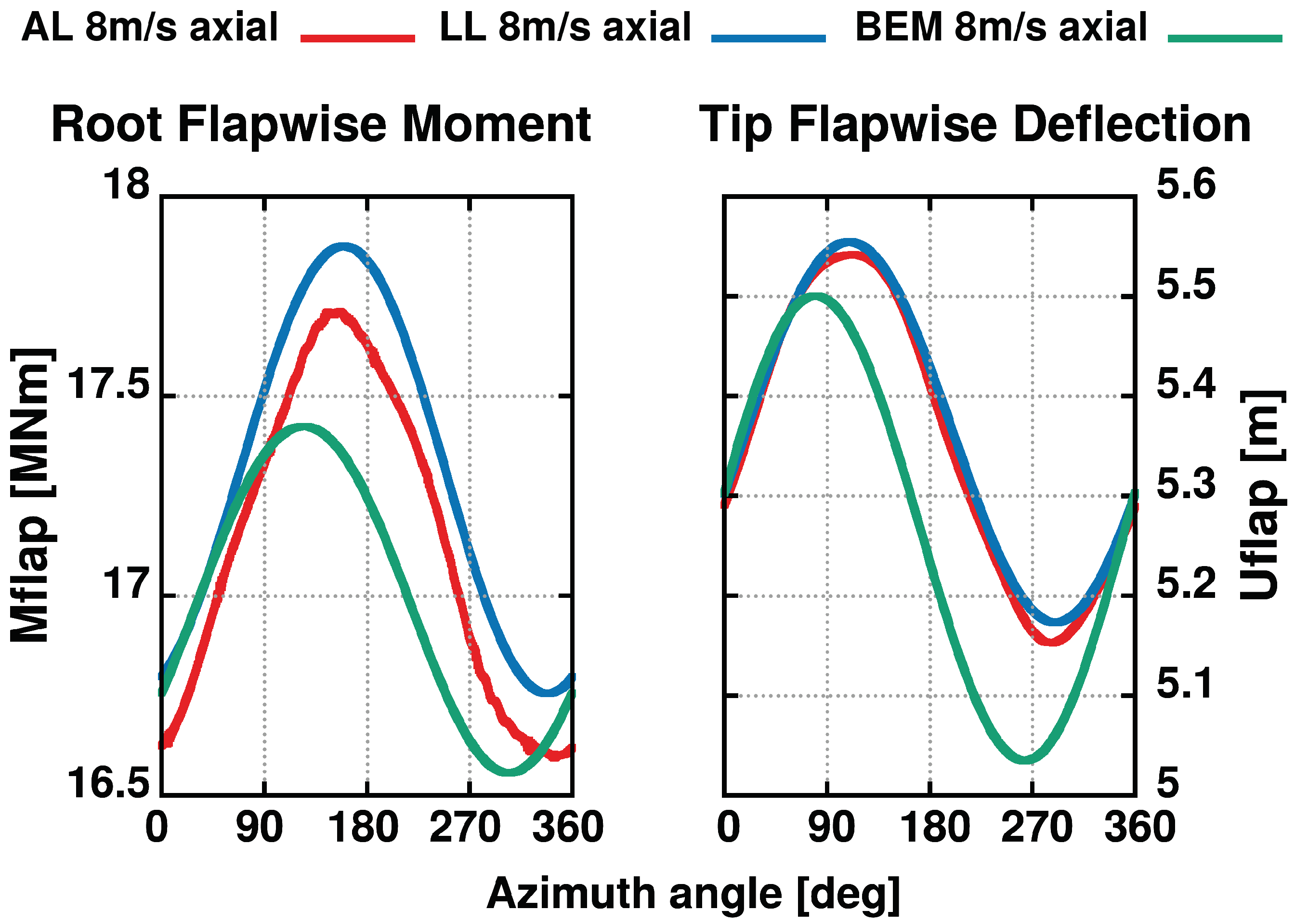
Figure 16.
Out-of-plane root bending moment and tip deflection at 8 m/s axial wind speed.
Figure 16.
Out-of-plane root bending moment and tip deflection at 8 m/s axial wind speed.
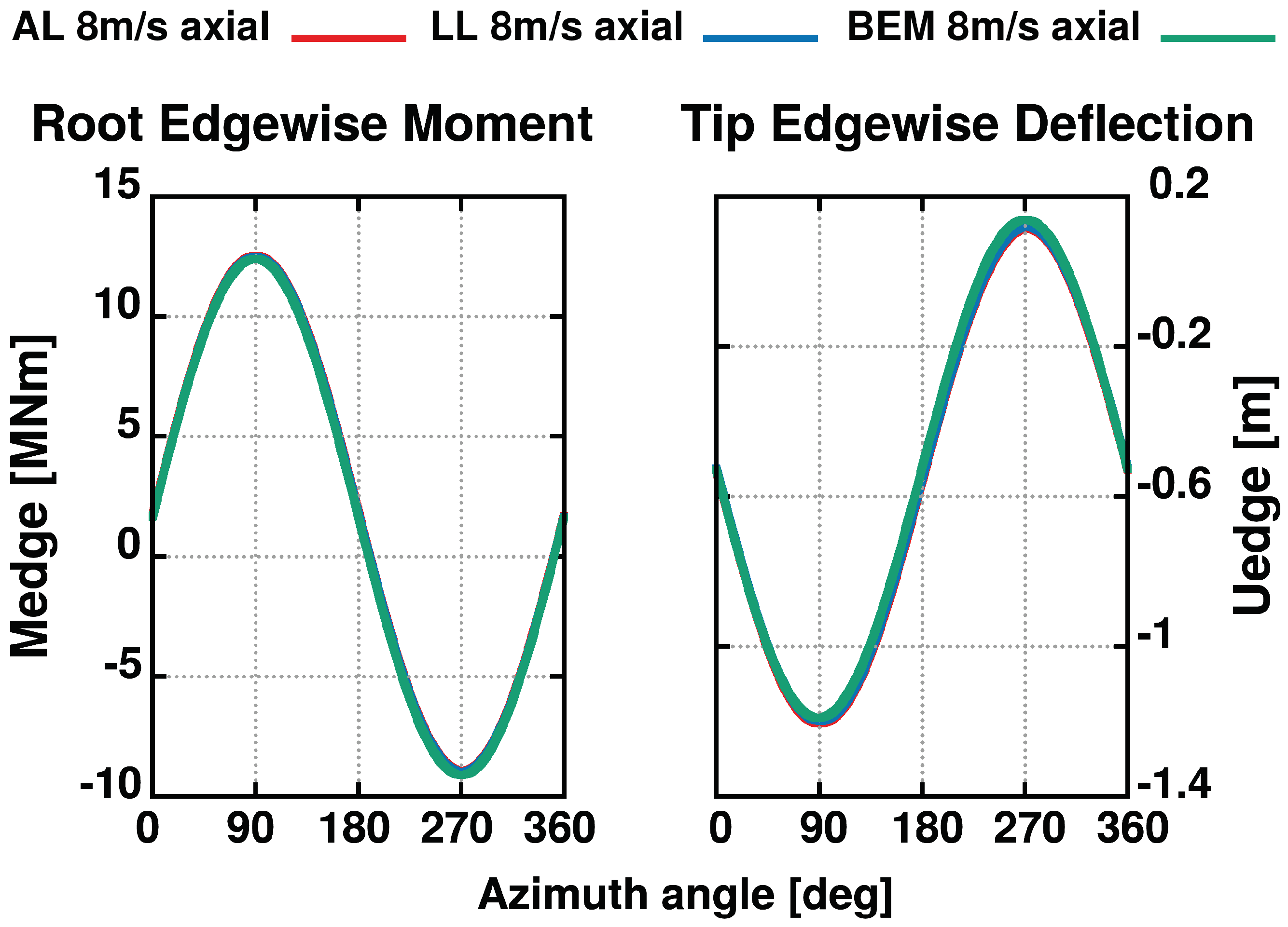
Figure 17.
In-plane root bending moment and tip deflection at 8 m/s axial wind speed.
Figure 17.
In-plane root bending moment and tip deflection at 8 m/s axial wind speed.
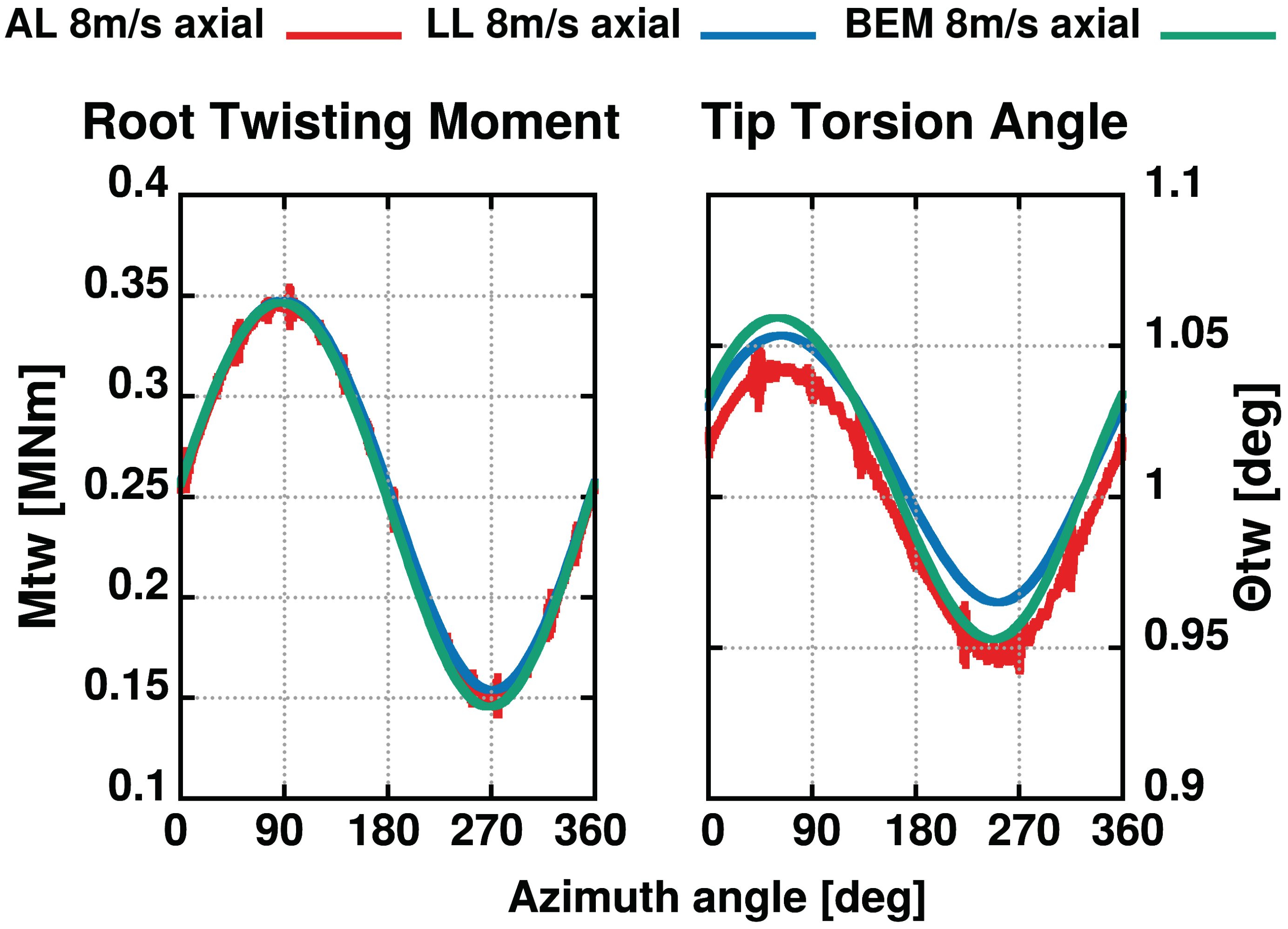
Figure 18.
Root twisting moment and tip torsion angle at 8 m/s axial wind speed.
Figure 18.
Root twisting moment and tip torsion angle at 8 m/s axial wind speed.
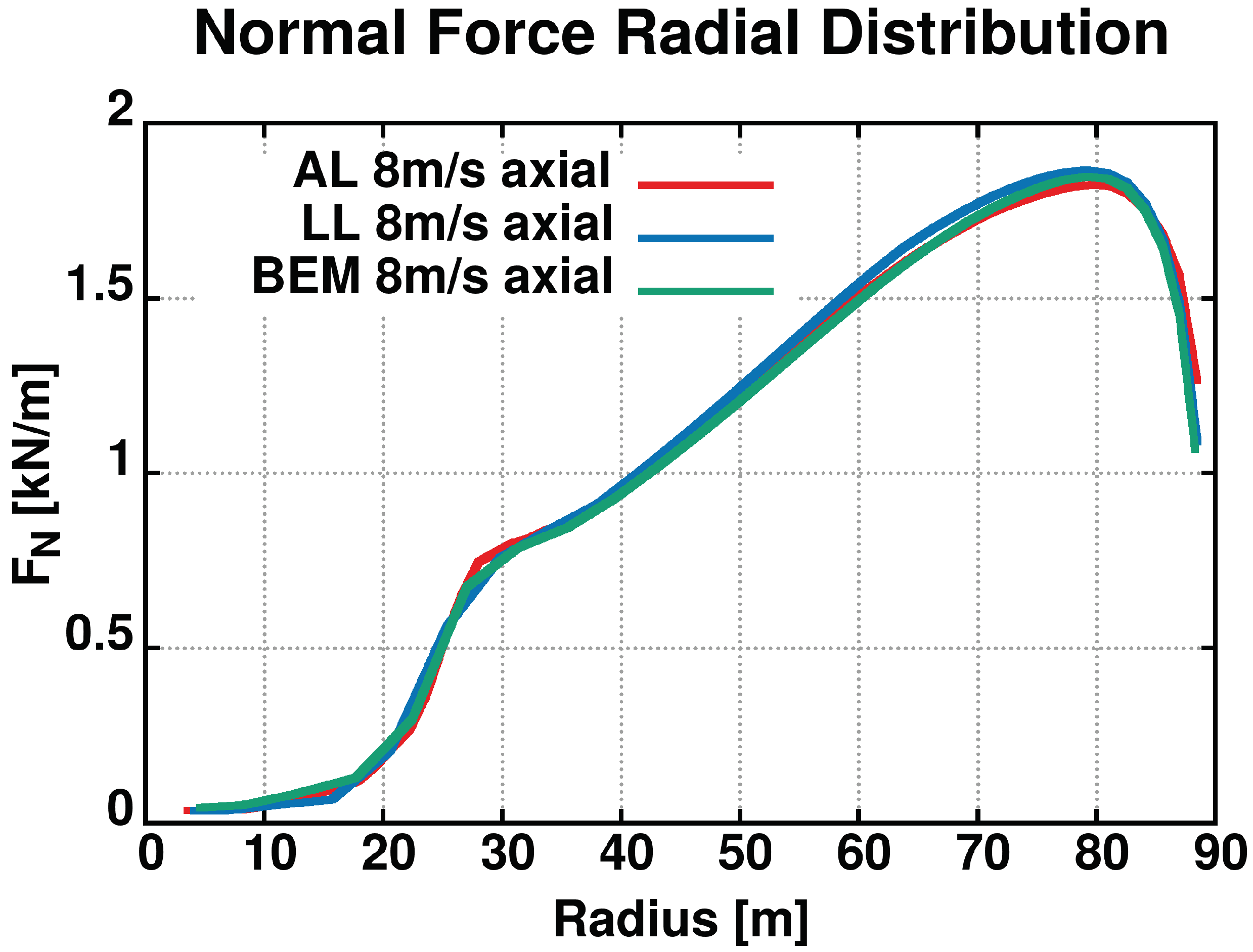
Figure 19.
Normal force radial distribution at 8 m/s axial wind speed. Averaging over the final revolution of the simulation.
Figure 19.
Normal force radial distribution at 8 m/s axial wind speed. Averaging over the final revolution of the simulation.
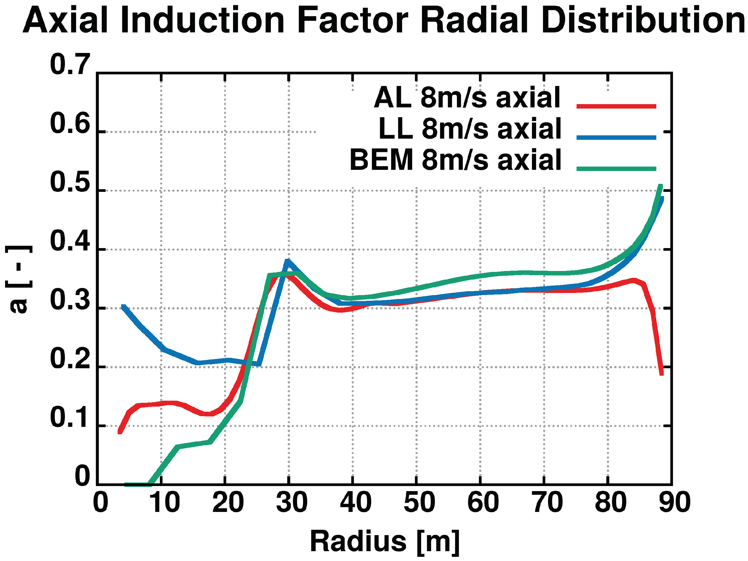
Figure 20.
Axial induction factor radial distribution at 8 m/s axial wind speed. Averaging over the final revolution of the simulation.
Figure 20.
Axial induction factor radial distribution at 8 m/s axial wind speed. Averaging over the final revolution of the simulation.
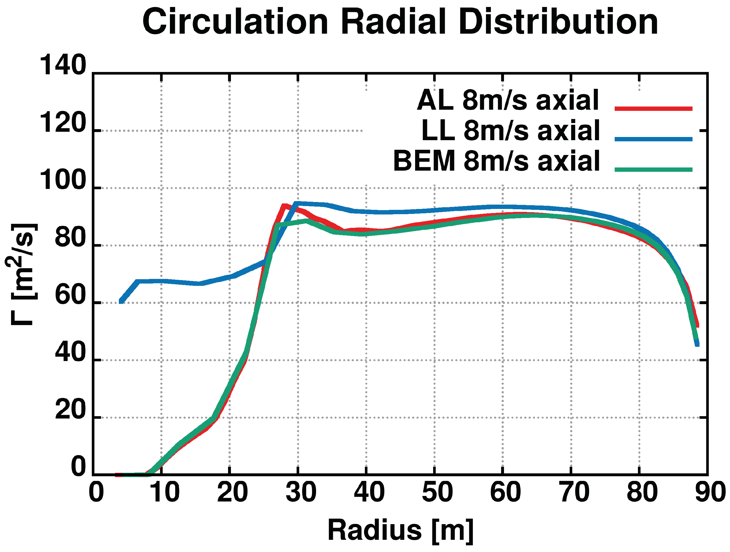
Figure 21.
Circulation radial distribution at 8 m/s axial wind speed. Averaging over the final revolution of the simulation.
Figure 21.
Circulation radial distribution at 8 m/s axial wind speed. Averaging over the final revolution of the simulation.
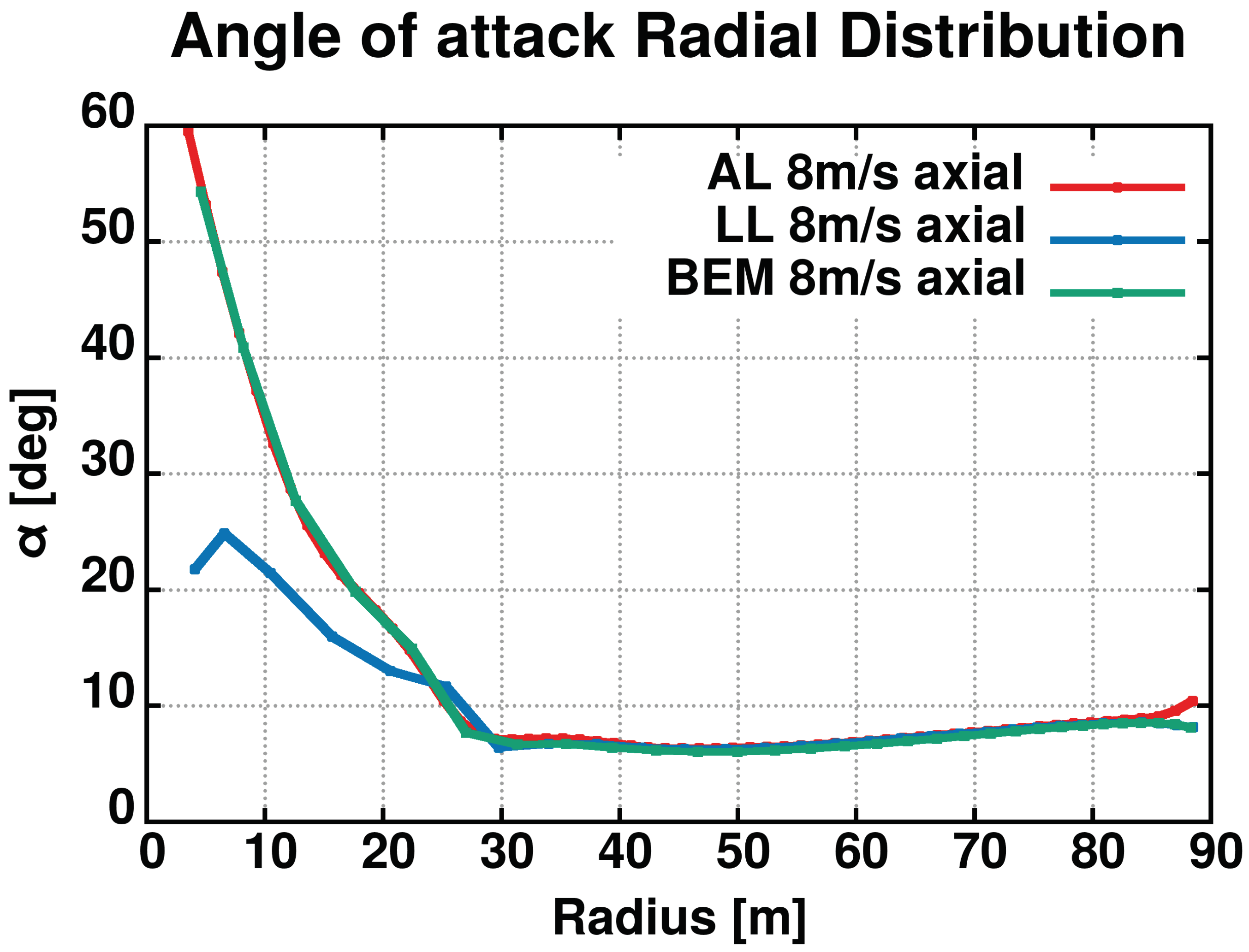
Figure 22.
Angle of attack radial distribution at 8 m/s axial wind speed. Averaging over the final revolution of the simulation.
Figure 22.
Angle of attack radial distribution at 8 m/s axial wind speed. Averaging over the final revolution of the simulation.
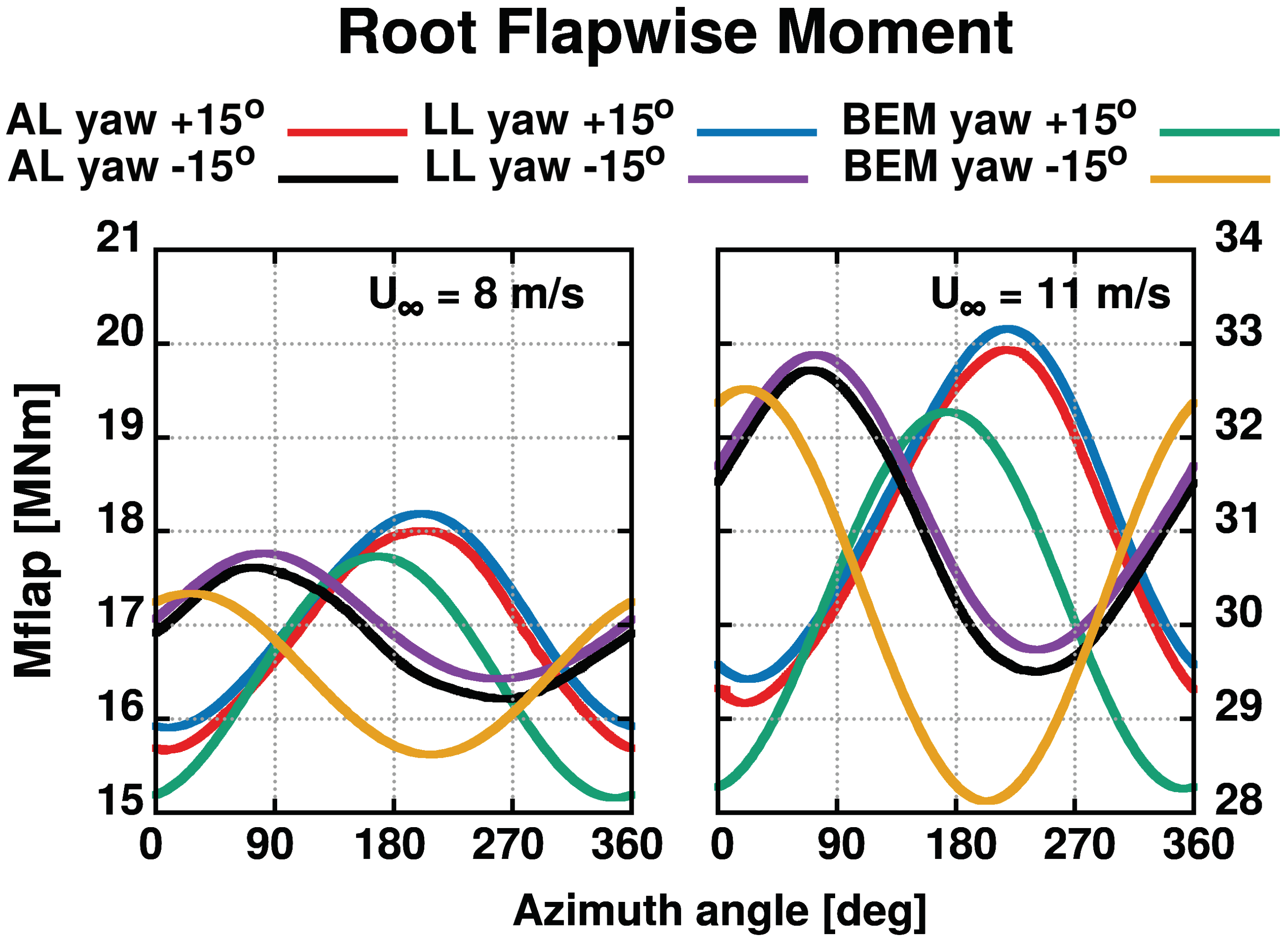
Figure 23.
Out-of-plane bending moment of blade root at 15 yawed wind speed at 8 and 11 m/s.
Figure 23.
Out-of-plane bending moment of blade root at 15 yawed wind speed at 8 and 11 m/s.
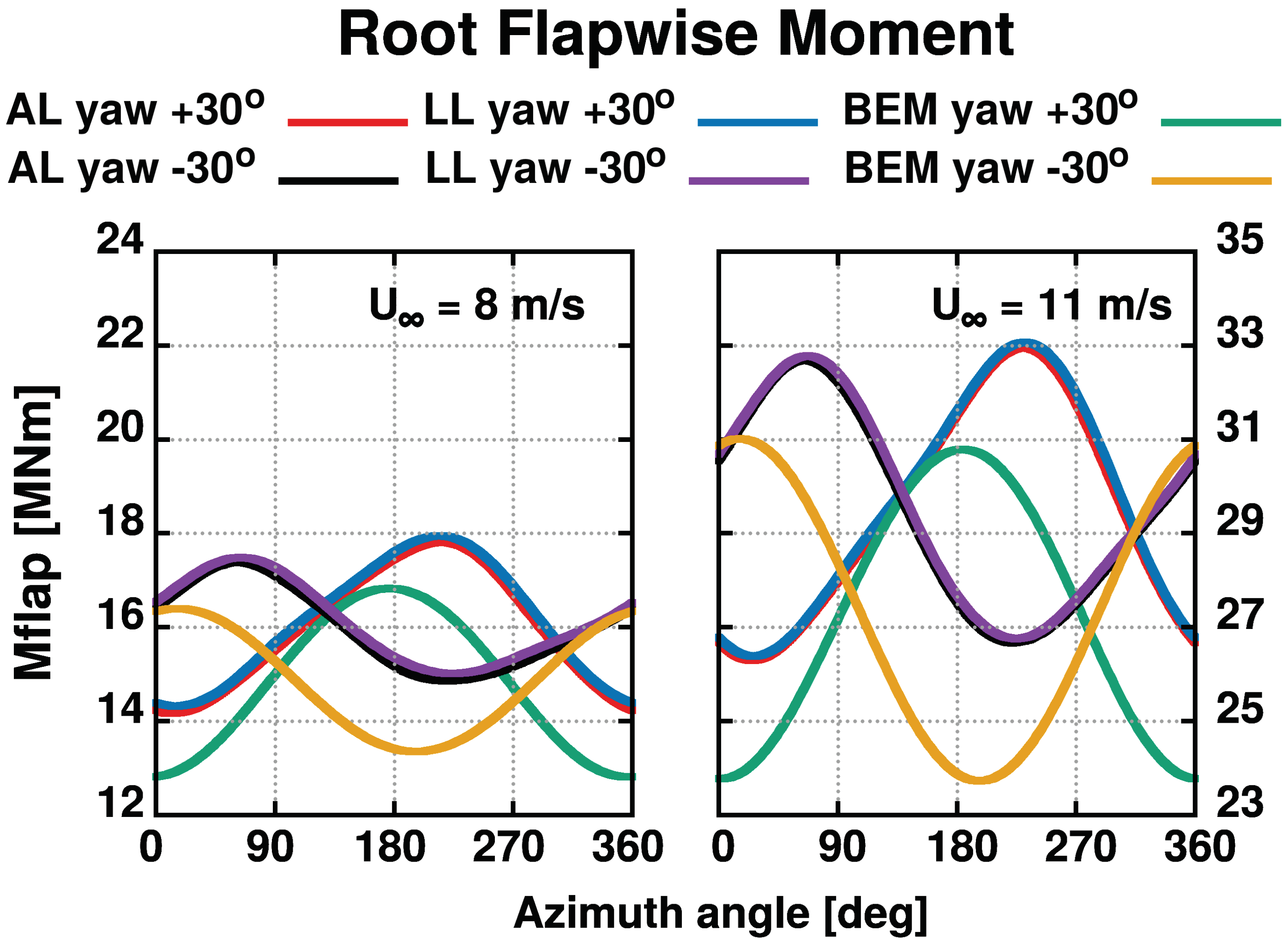
Figure 24.
Out-of-plane bending moment of blade root at 30 yawed wind speed at 8 and 11 m/s.
Figure 24.
Out-of-plane bending moment of blade root at 30 yawed wind speed at 8 and 11 m/s.
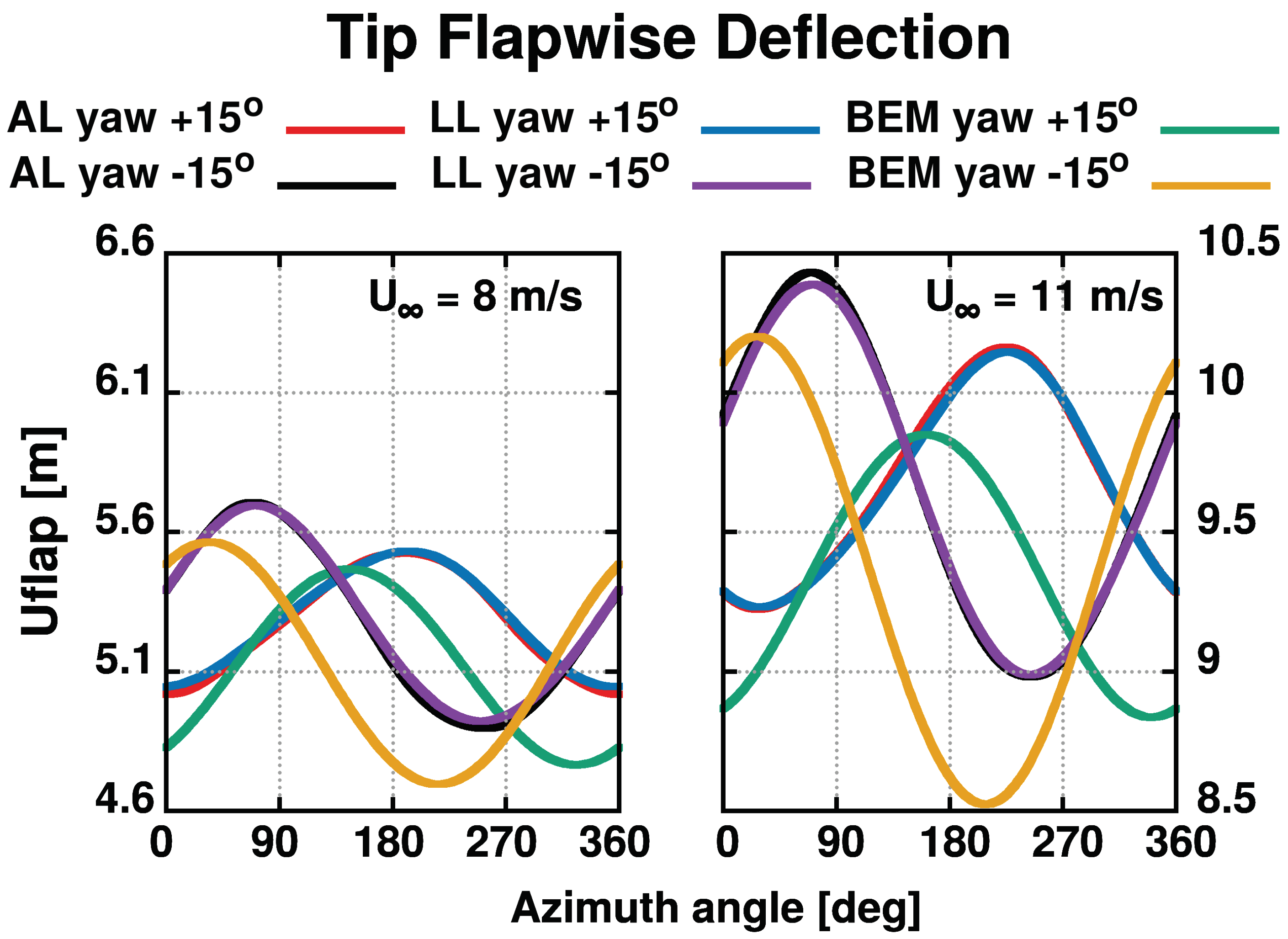
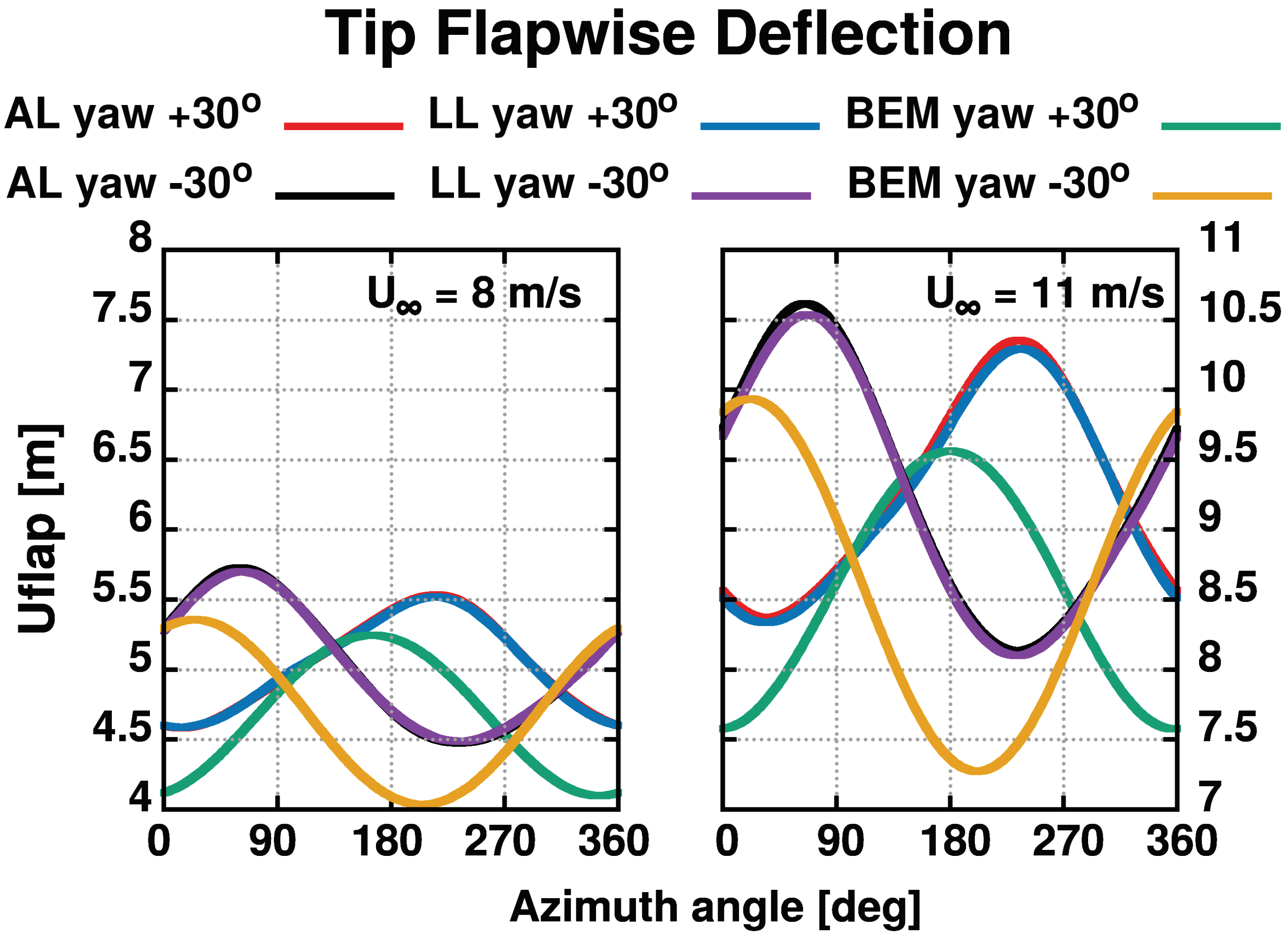
Figure 25.
Out-of-plane deflection of blade tip at 15 yawed wind speed at 8 and 11 m/s.
Figure 25.
Out-of-plane deflection of blade tip at 15 yawed wind speed at 8 and 11 m/s.
Figure 26.
Out-of-plane deflection of blade tip at 30 yawed wind speed at 8 and 11 m/s.
Figure 26.
Out-of-plane deflection of blade tip at 30 yawed wind speed at 8 and 11 m/s.
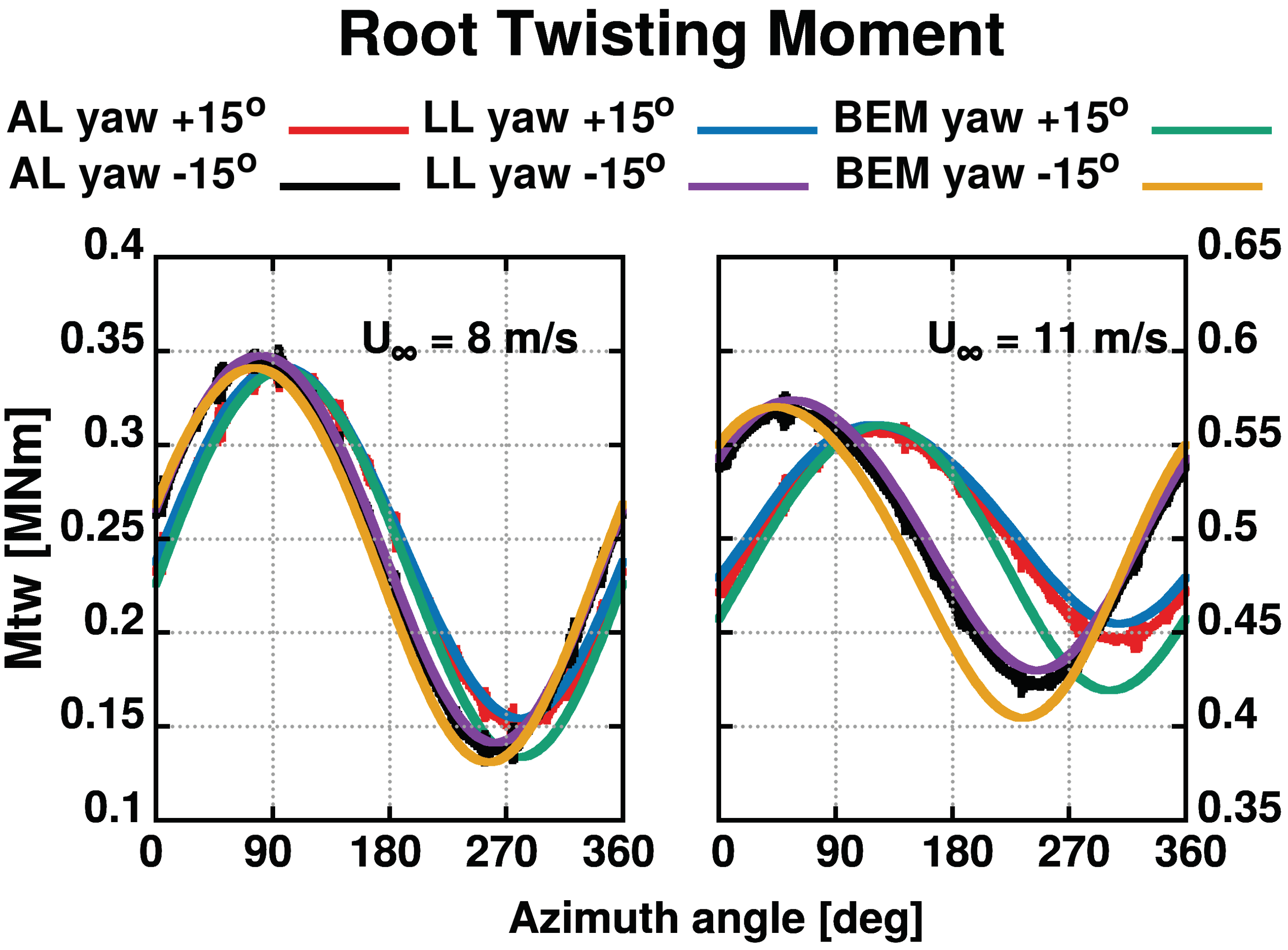
Figure 27.
Twisting moment of blade root at 15 yawed wind speed at 8 and 11 m/s.
Figure 27.
Twisting moment of blade root at 15 yawed wind speed at 8 and 11 m/s.
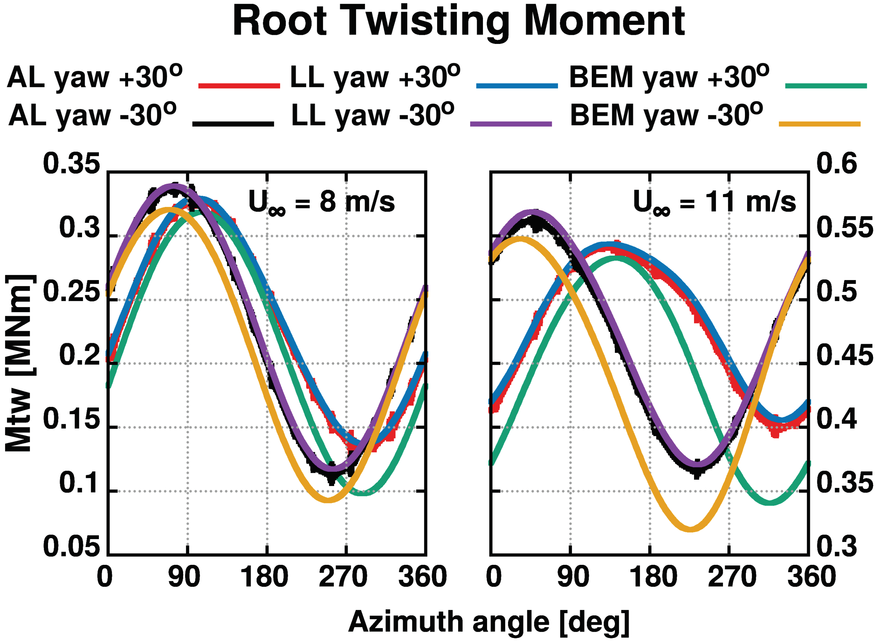
Figure 28.
Twisting moment of blade root at 30 yawed wind speed at 8 and 11 m/s.
Figure 28.
Twisting moment of blade root at 30 yawed wind speed at 8 and 11 m/s.
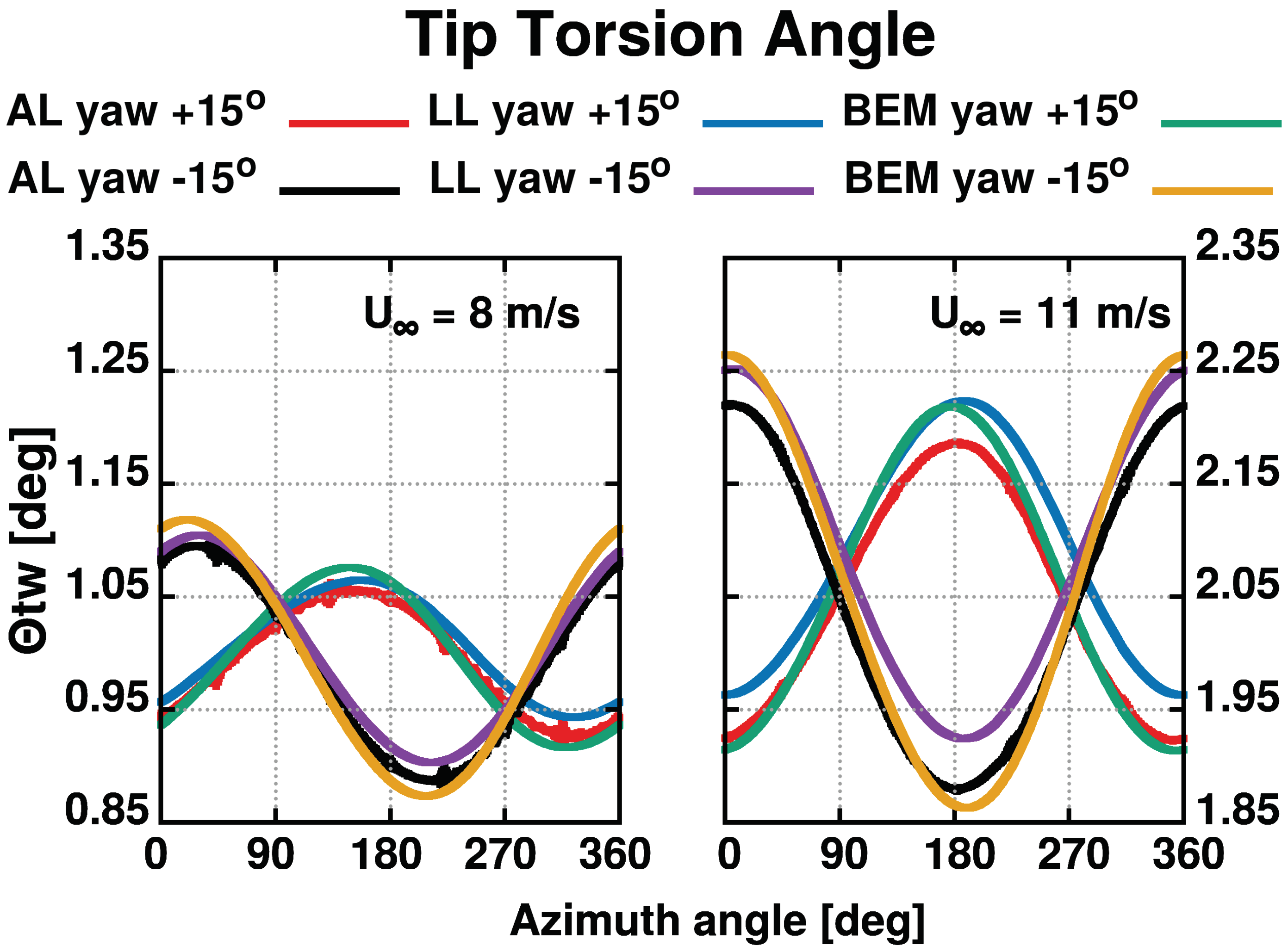
Figure 29.
Torsion angle of blade tip at 15 yawed wind speed at 8 and 11 m/s.
Figure 29.
Torsion angle of blade tip at 15 yawed wind speed at 8 and 11 m/s.
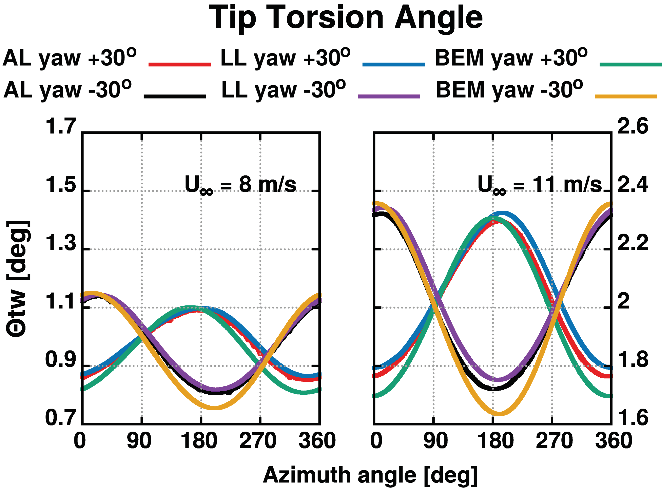
Figure 30.
Torsion angle of blade tip at 30 yawed wind speed at 8 and 11 m/s.
Figure 30.
Torsion angle of blade tip at 30 yawed wind speed at 8 and 11 m/s.
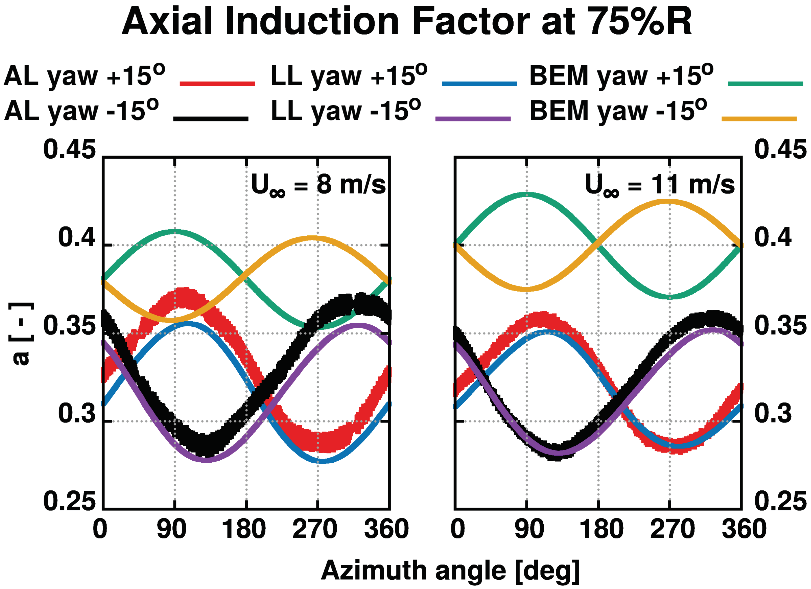
Figure 31.
Axial induction factor at of the blade at 15 yawed wind speed at 8 and 11 m/s.
Figure 31.
Axial induction factor at of the blade at 15 yawed wind speed at 8 and 11 m/s.
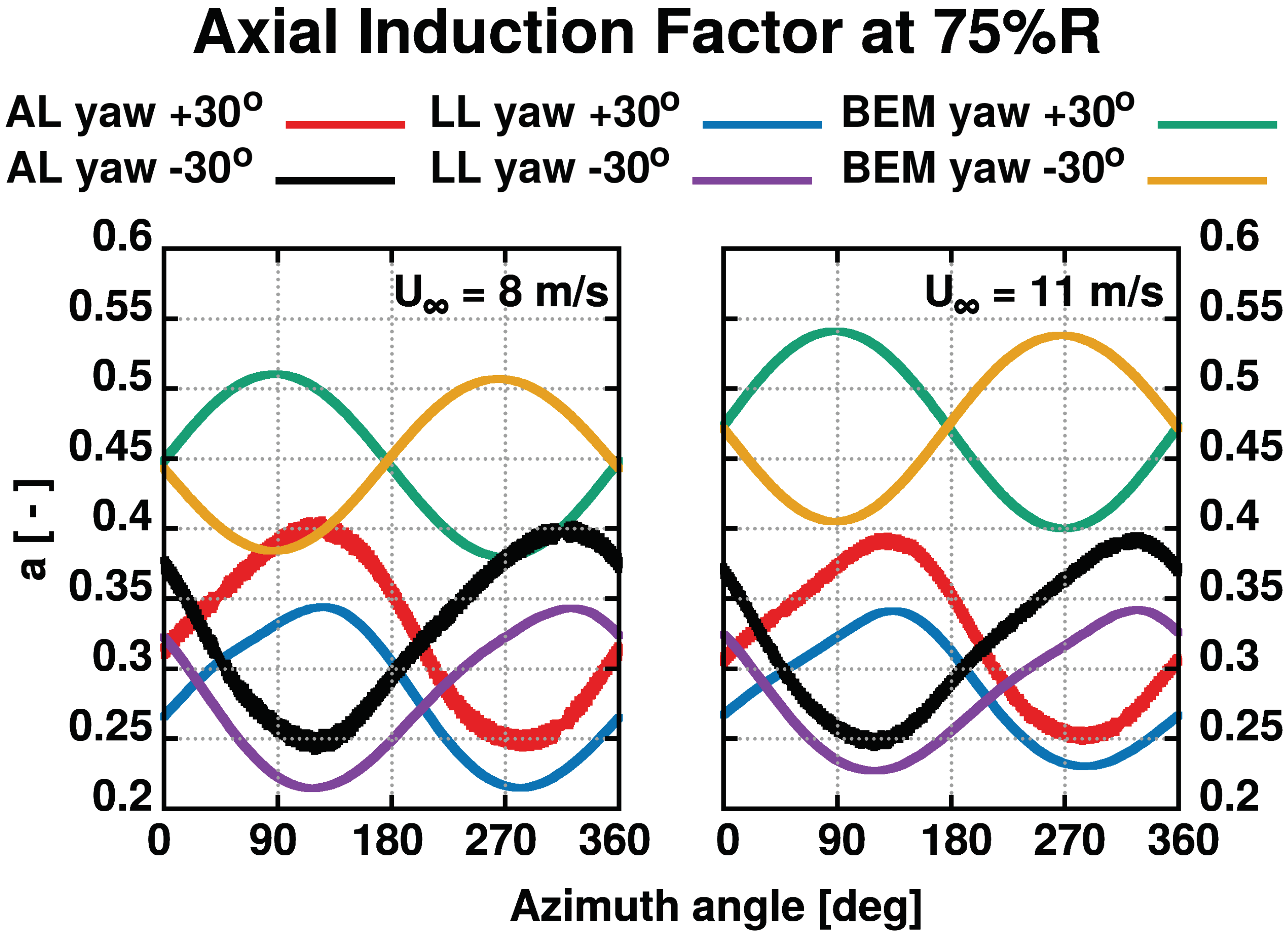
Figure 32.
Axial induction factor at of the blade at 30 yawed wind speed at 8 and 11 m/s.
Figure 32.
Axial induction factor at of the blade at 30 yawed wind speed at 8 and 11 m/s.
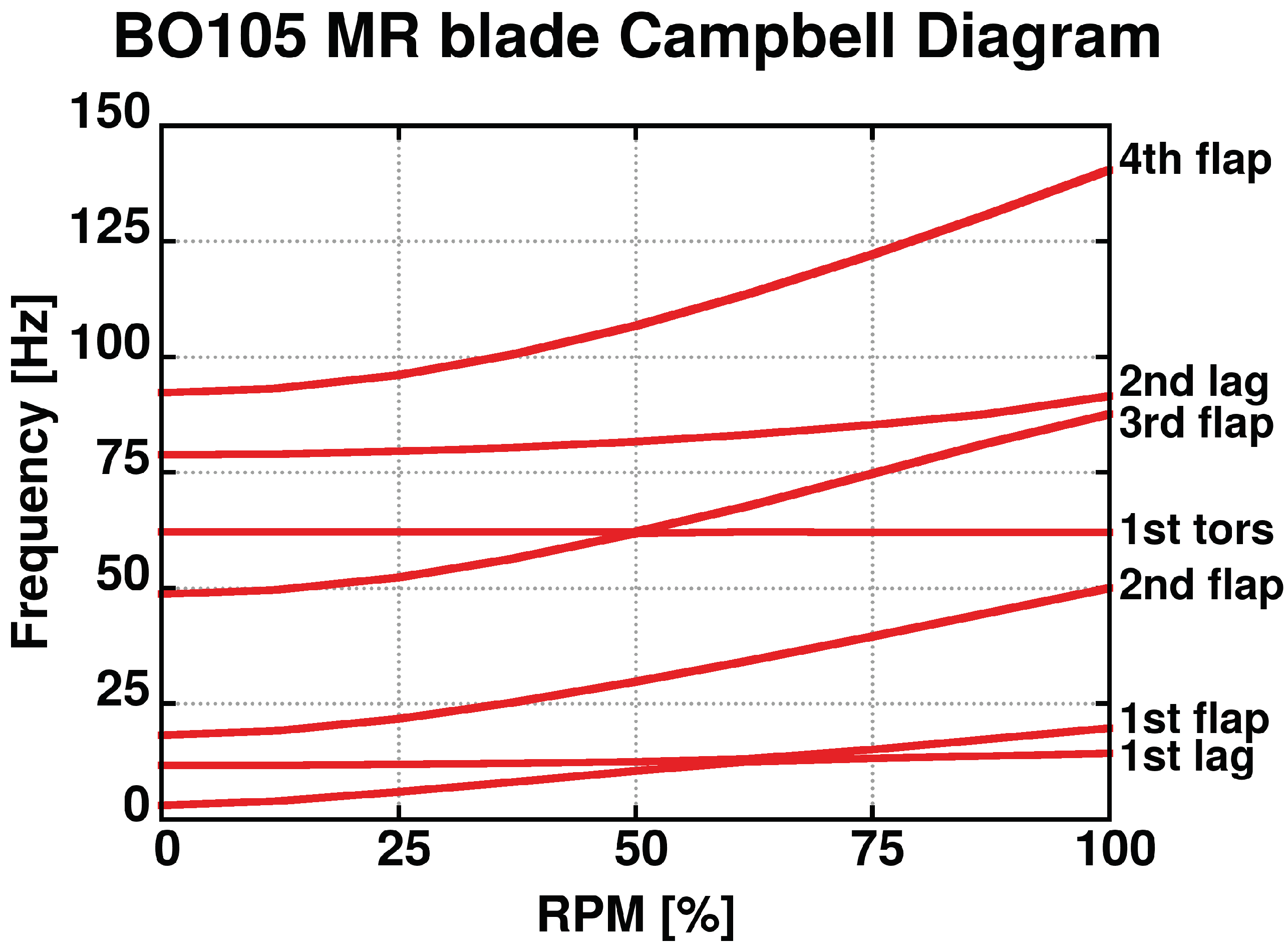
Figure 33.
Campbell diagram of BO105 MR.
Figure 33.
Campbell diagram of BO105 MR.
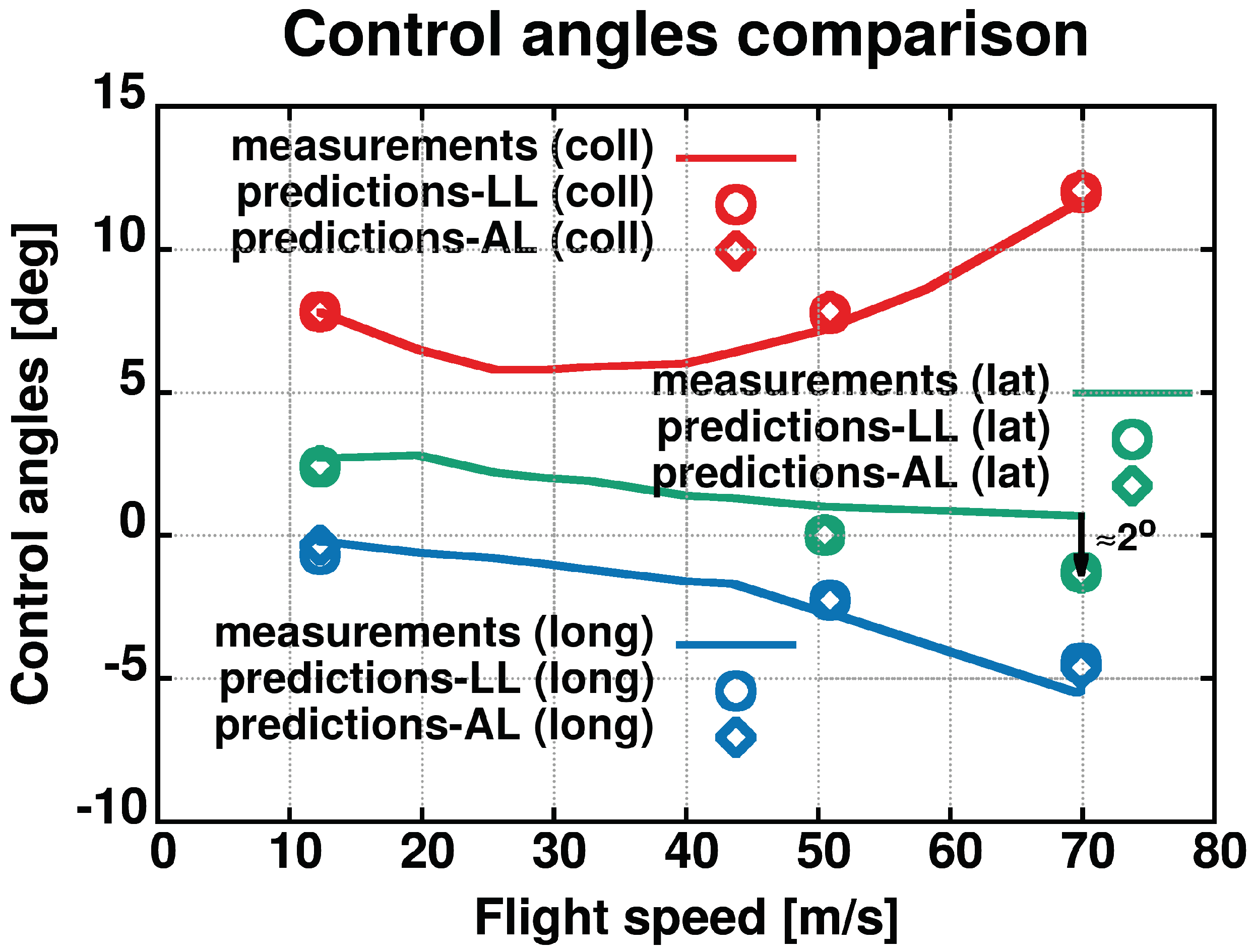
Figure 34.
Control angles comparison. Trimmed simulation values vs experimental measurements.
Figure 34.
Control angles comparison. Trimmed simulation values vs experimental measurements.
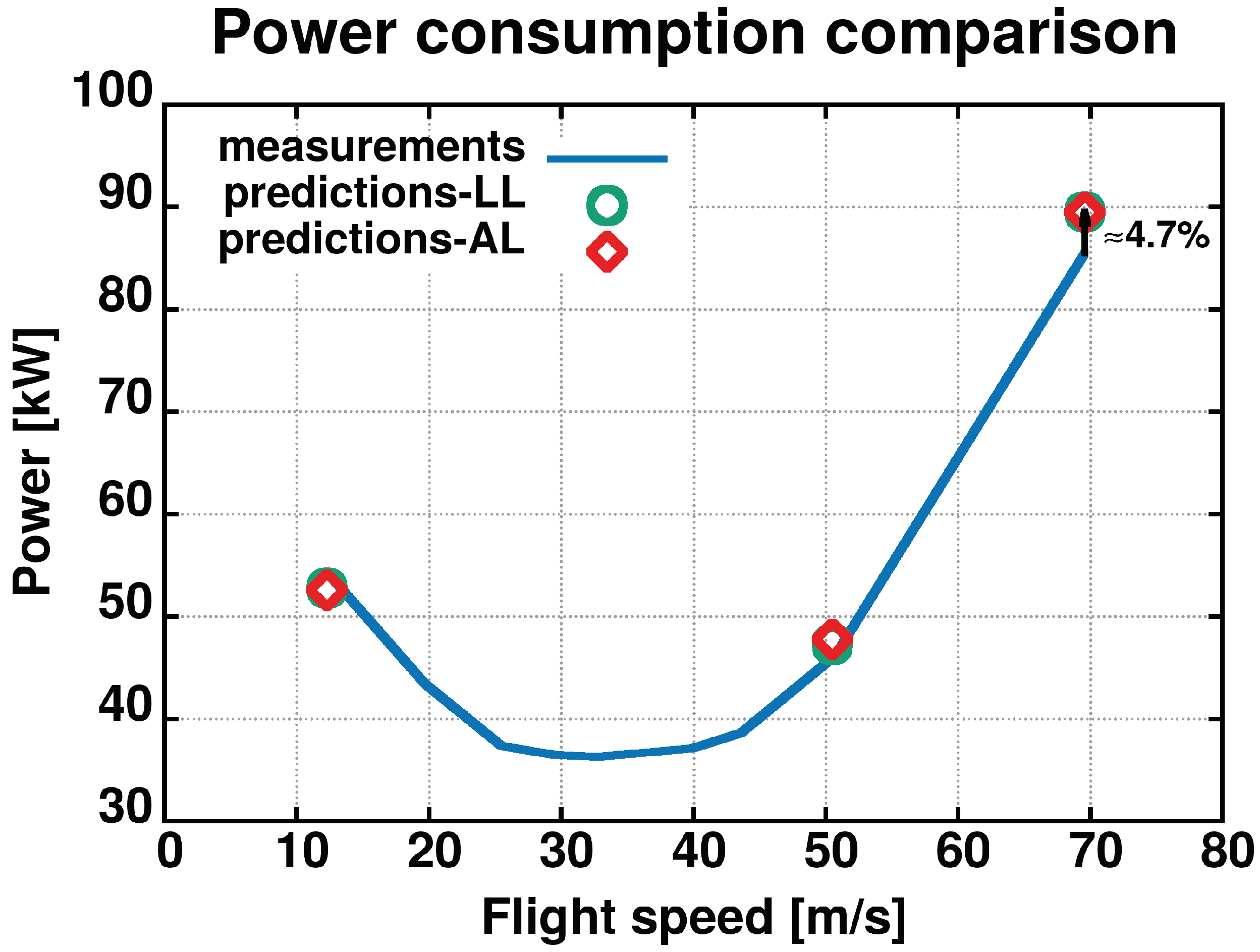
Figure 35.
Rotor power requirement comparison. Simulation predictions vs experimental measurements.
Figure 35.
Rotor power requirement comparison. Simulation predictions vs experimental measurements.
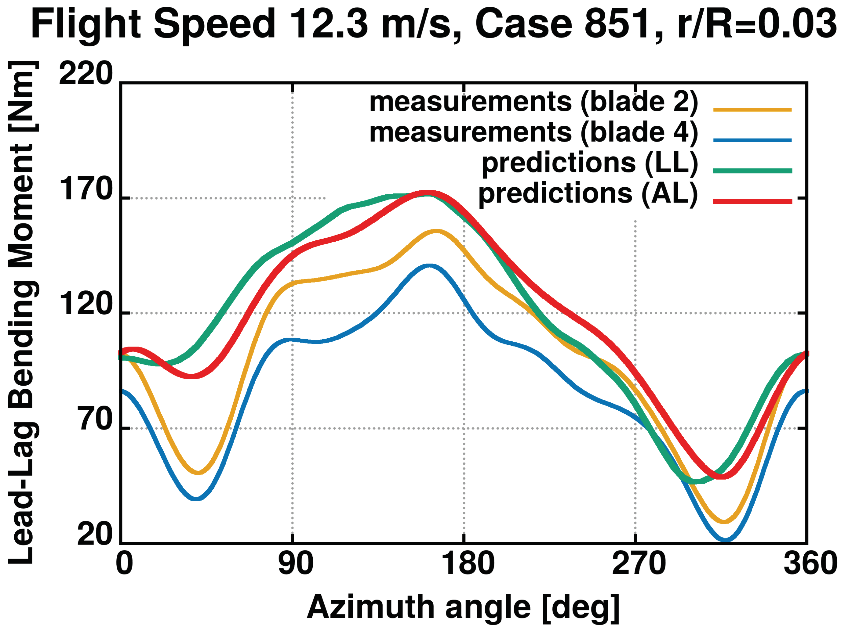
Figure 36.
Forward flight at 12.3 m/s, case 851. Lead-lag moment at .
Figure 36.
Forward flight at 12.3 m/s, case 851. Lead-lag moment at .
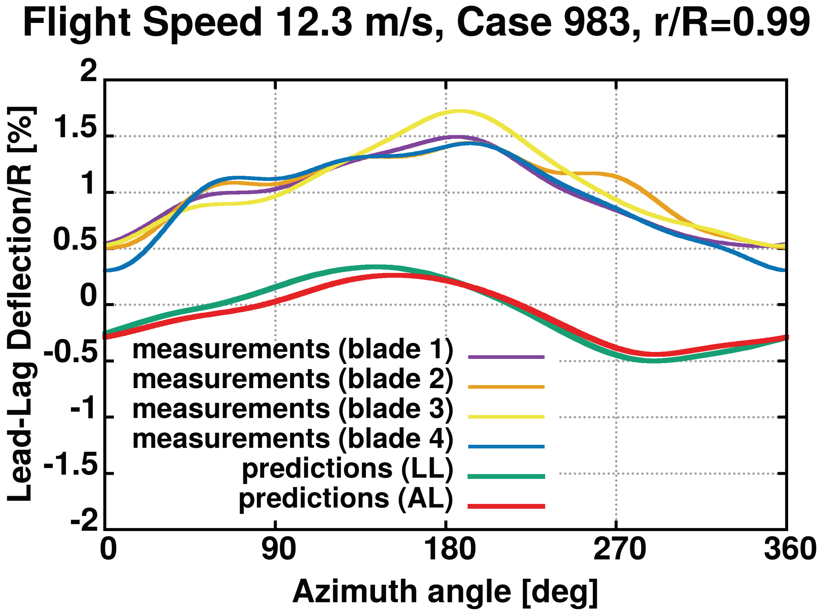
Figure 37.
Forward flight at 12.3 m/s, case 983. Lead-lag deflection at .
Figure 37.
Forward flight at 12.3 m/s, case 983. Lead-lag deflection at .
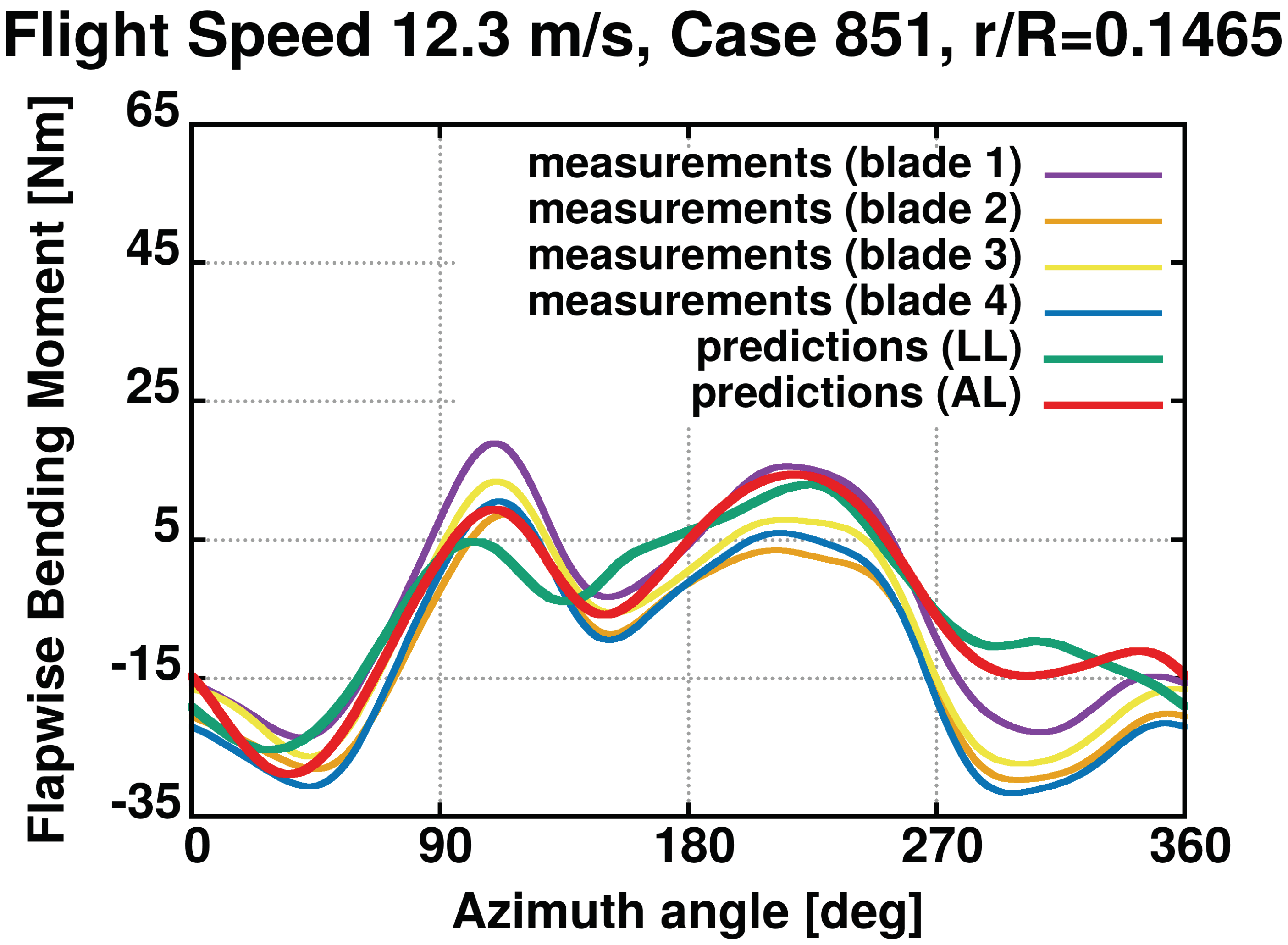
Figure 38.
Forward flight at 12.3 m/s, case 851. Flapwise moment at .
Figure 38.
Forward flight at 12.3 m/s, case 851. Flapwise moment at .
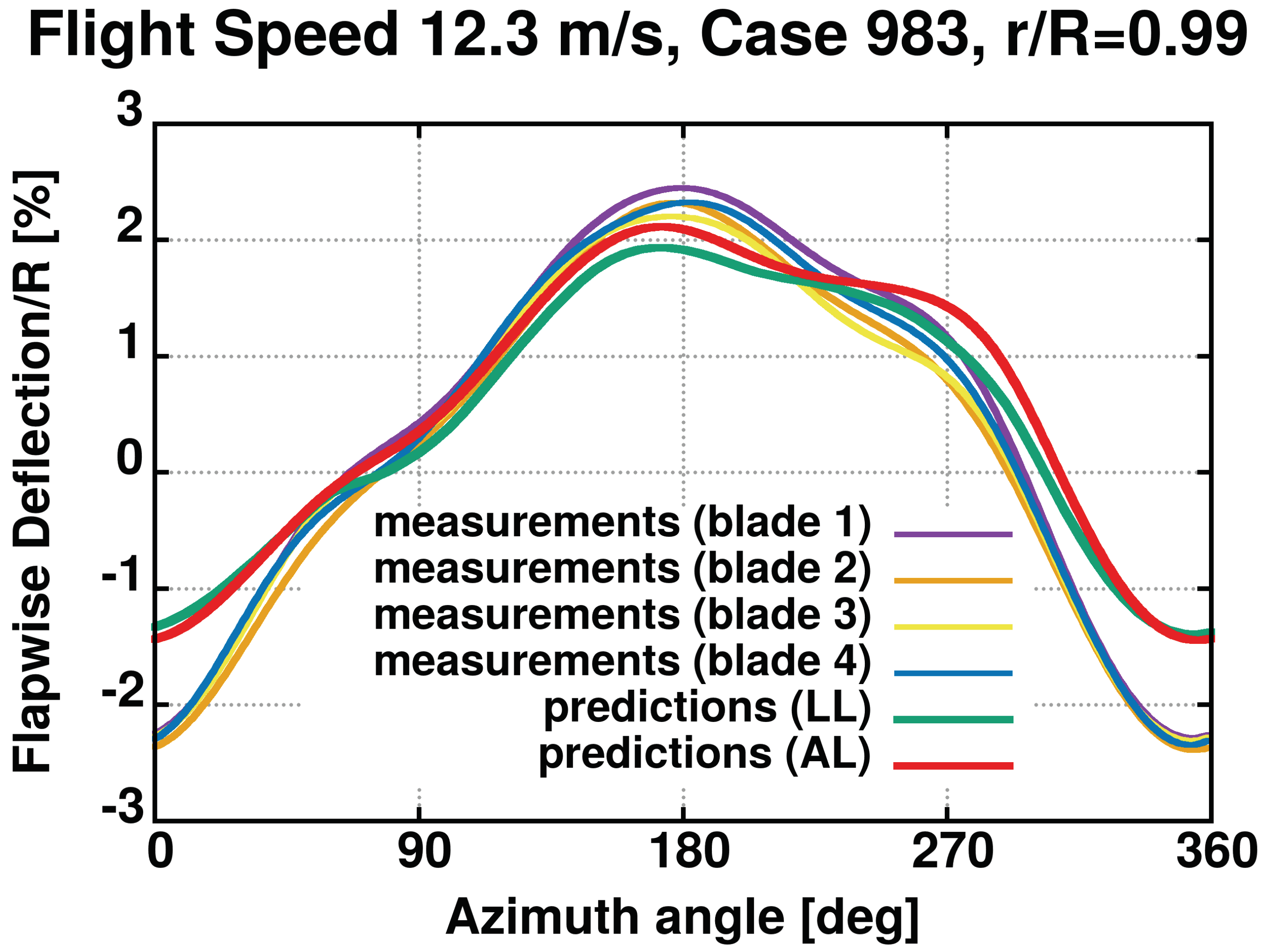
Figure 39.
Forward flight at 12.3 m/s, case 983. Flapwise deflection at .
Figure 39.
Forward flight at 12.3 m/s, case 983. Flapwise deflection at .
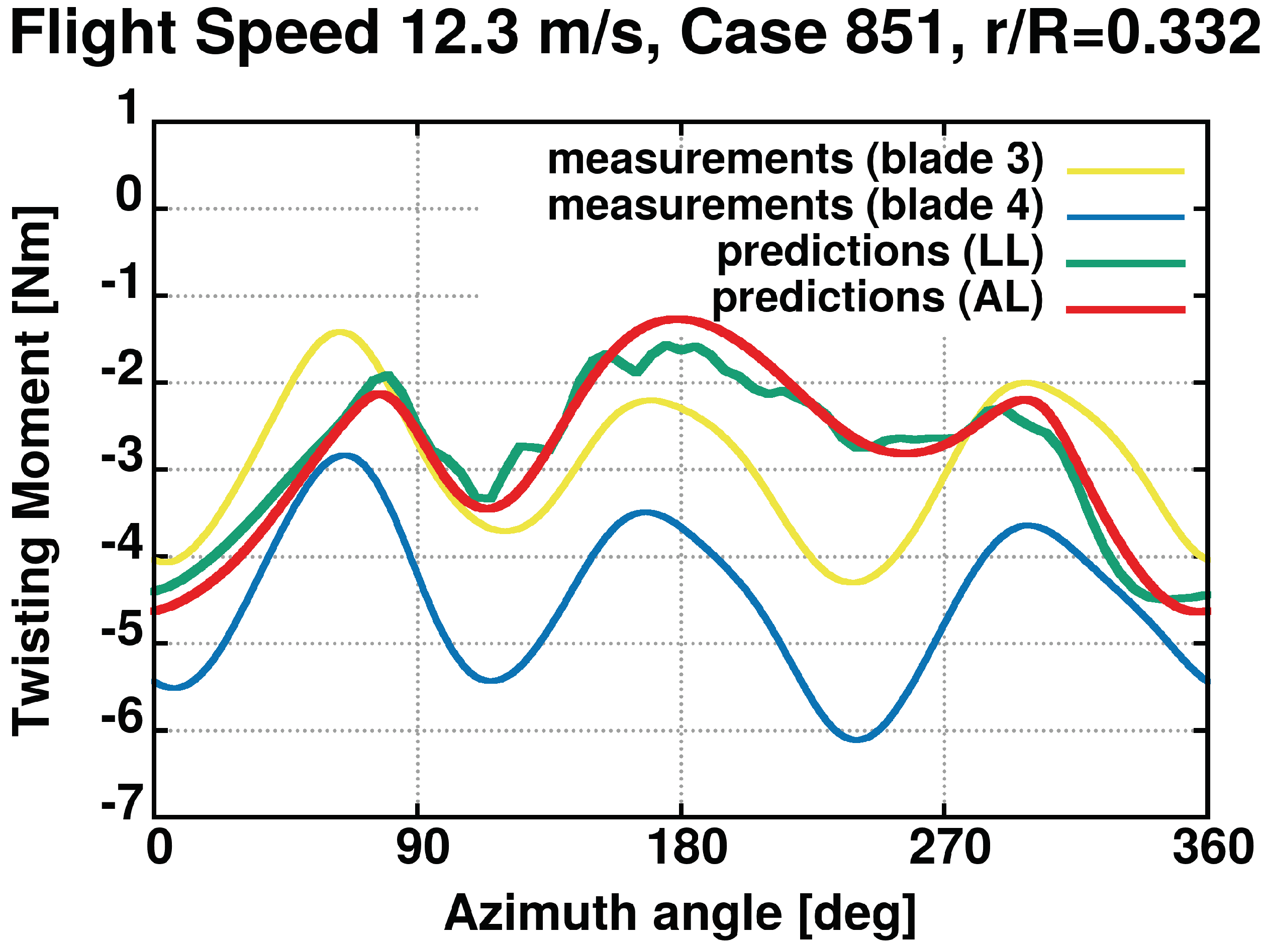
Figure 40.
Forward flight at 12.3 m/s, case 851. Twisting moment at .
Figure 40.
Forward flight at 12.3 m/s, case 851. Twisting moment at .
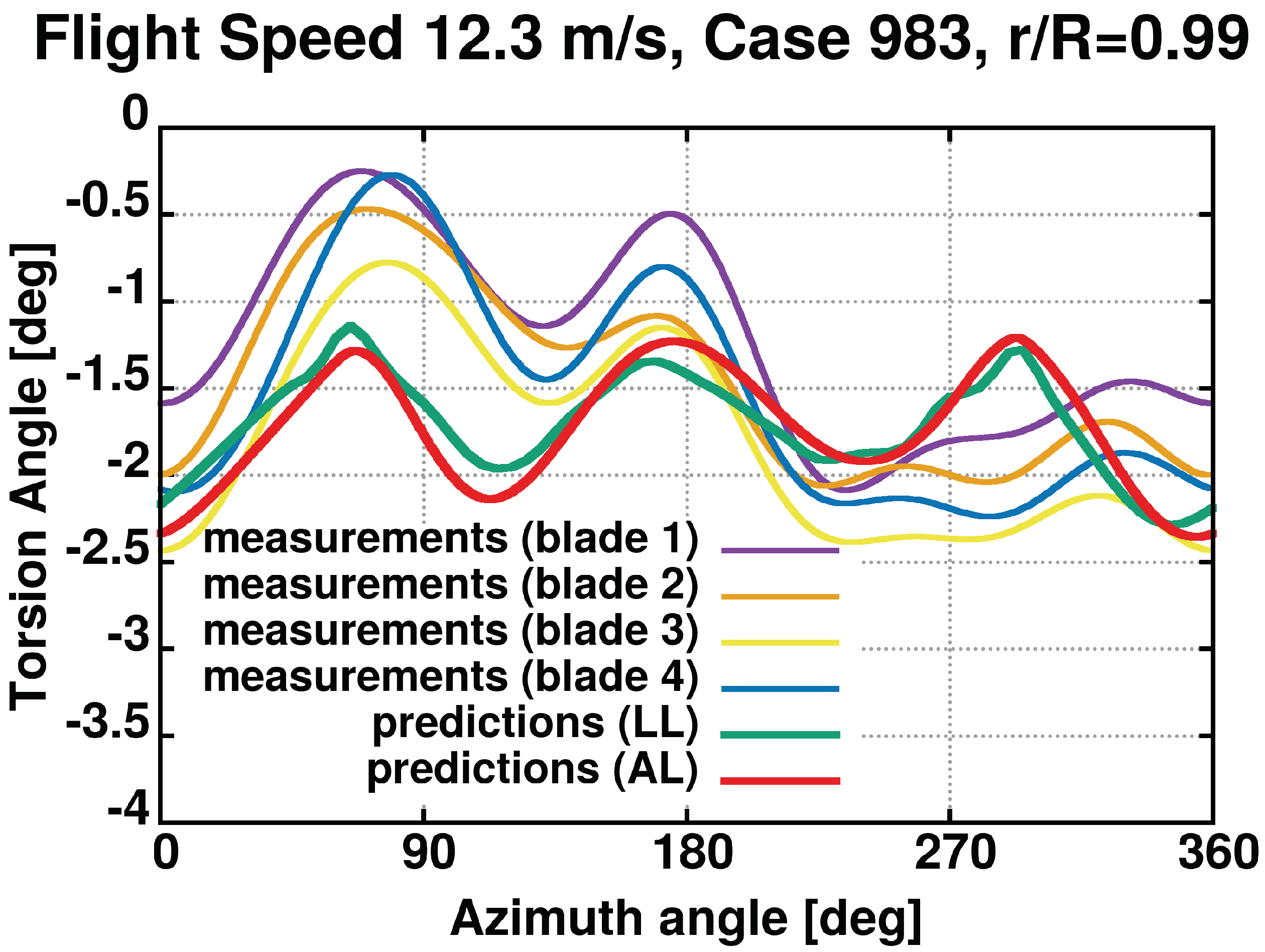
Figure 41.
Forward flight at 12.3 m/s, case 983. Torsion angle at .
Figure 41.
Forward flight at 12.3 m/s, case 983. Torsion angle at .
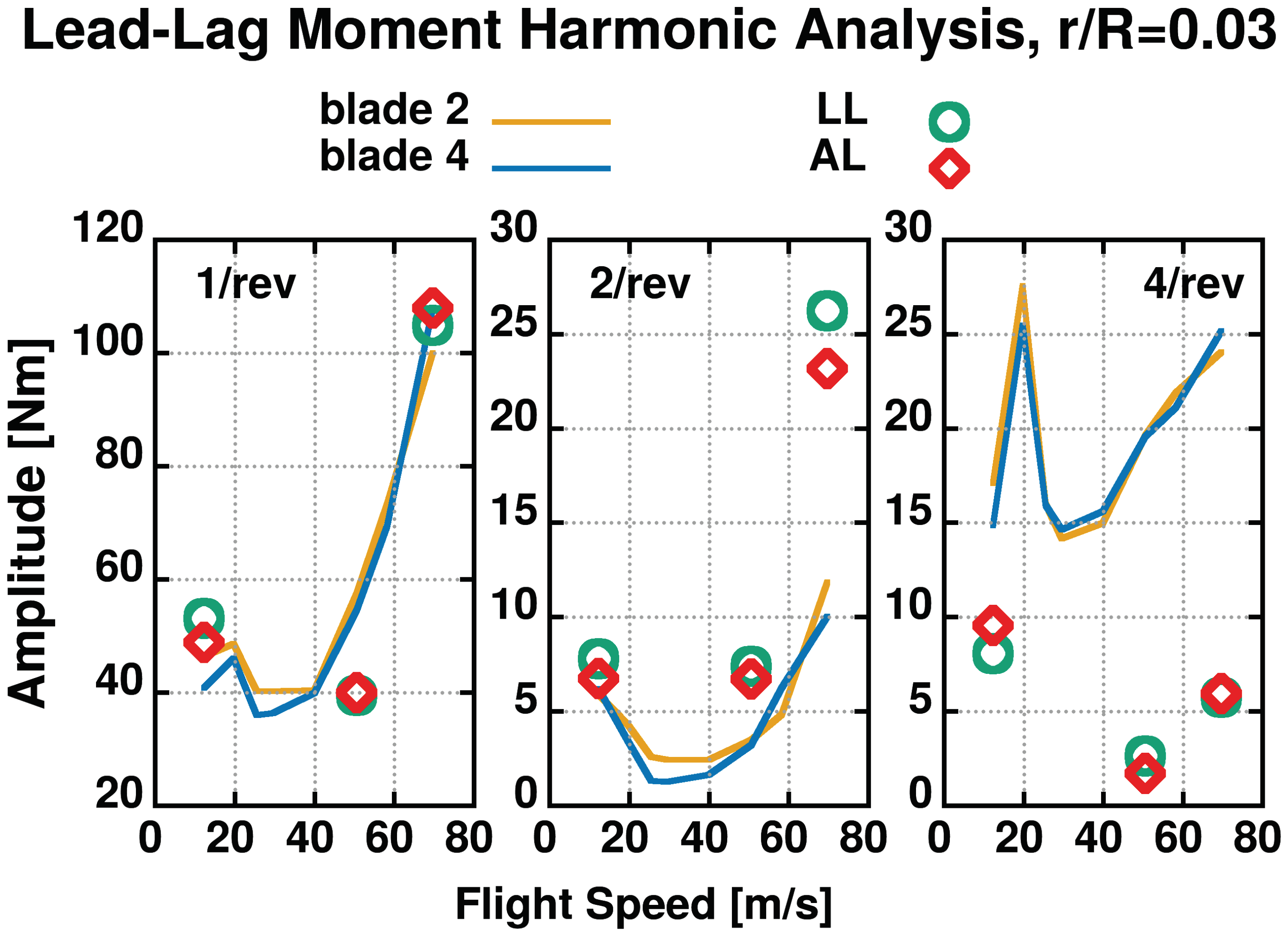
Figure 42.
Harmonic analysis of Lead-Lag bending moment. Amplitude of frequencies with the highest energy content.
Figure 42.
Harmonic analysis of Lead-Lag bending moment. Amplitude of frequencies with the highest energy content.
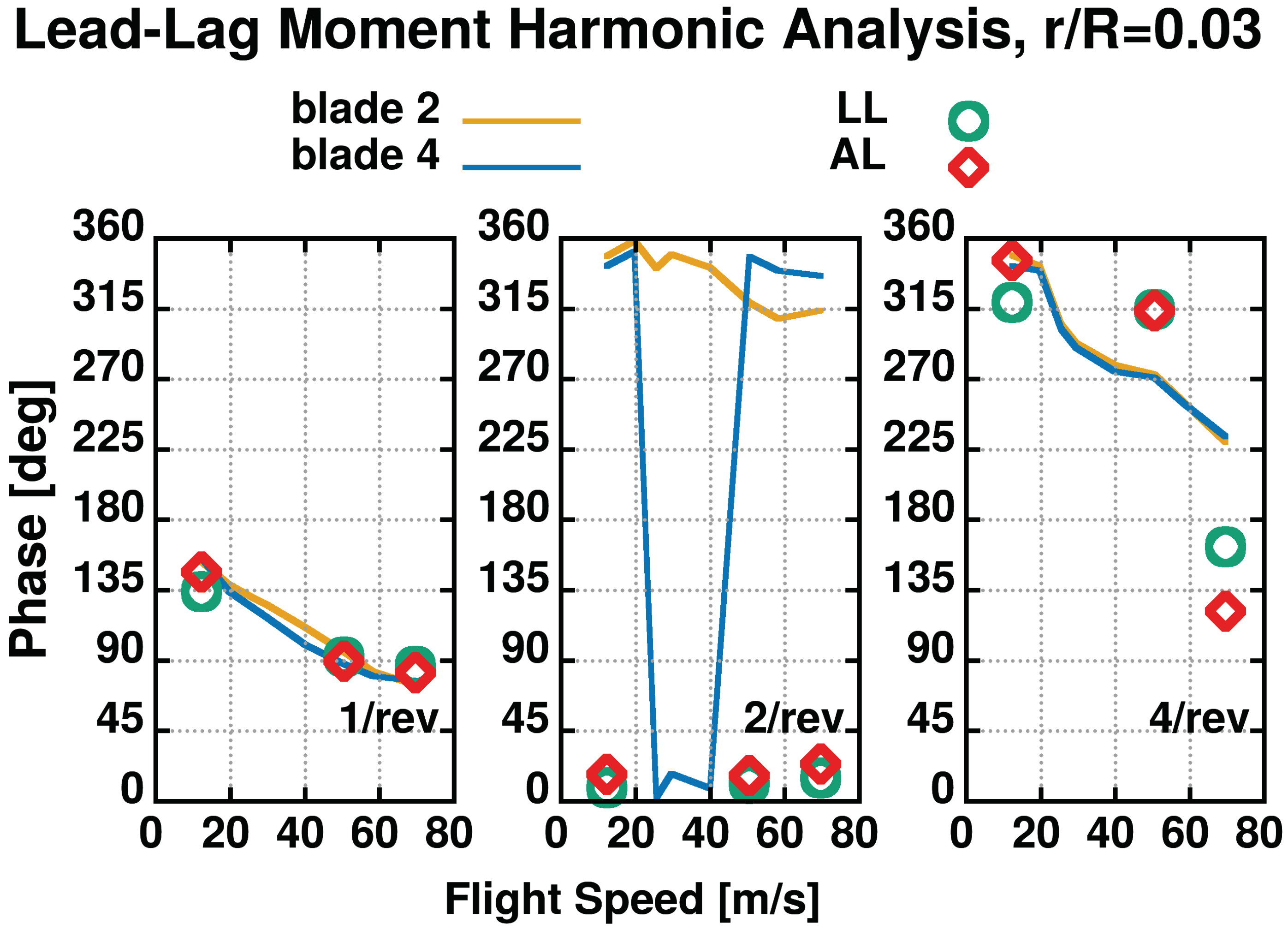
Figure 43.
Harmonic analysis of Lead-Lag bending moment. Phase of frequencies with the highest energy content.
Figure 43.
Harmonic analysis of Lead-Lag bending moment. Phase of frequencies with the highest energy content.
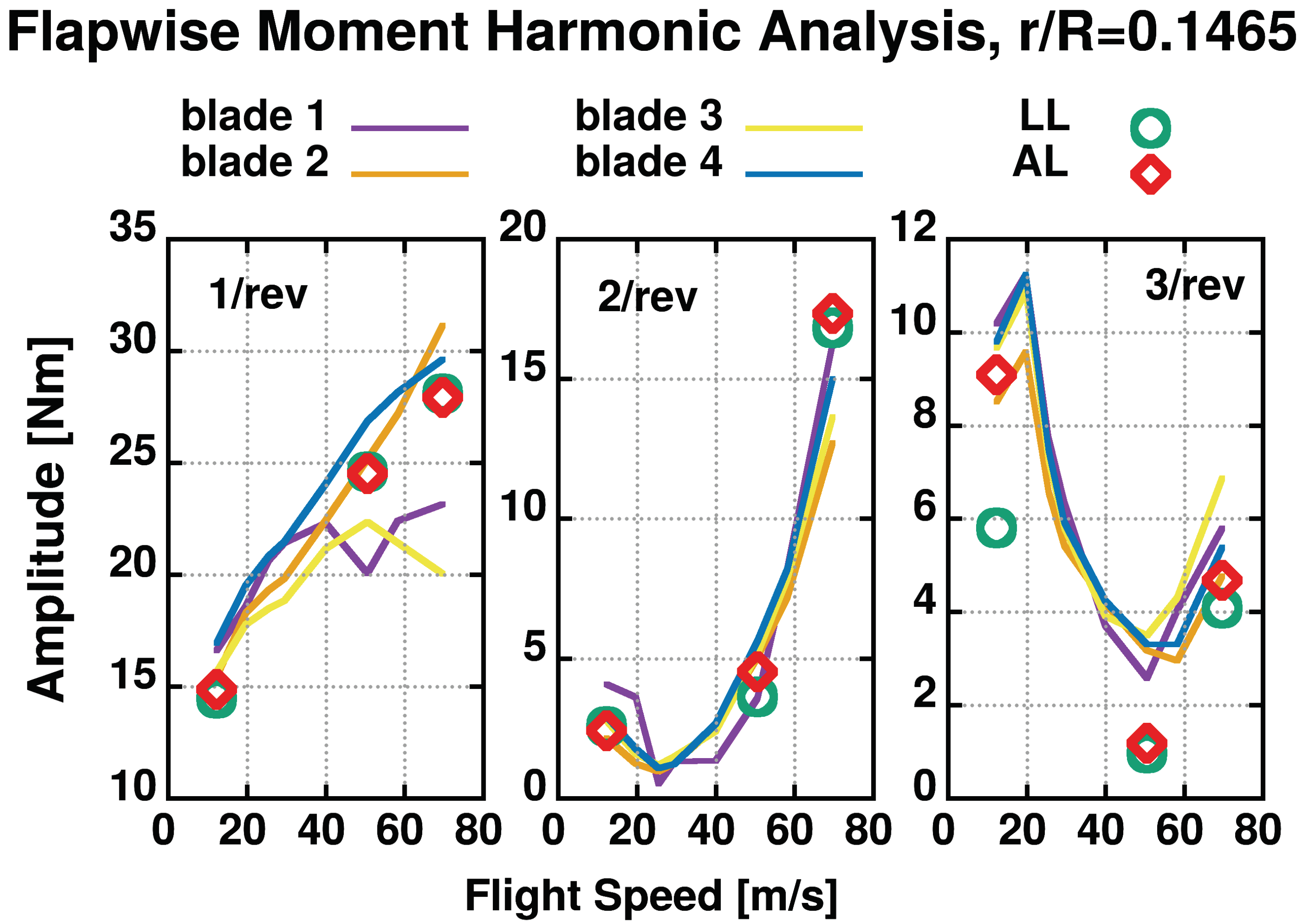
Figure 44.
Harmonic analysis of Flapwise bending moment. Amplitude of frequencies with the highest energy content.
Figure 44.
Harmonic analysis of Flapwise bending moment. Amplitude of frequencies with the highest energy content.
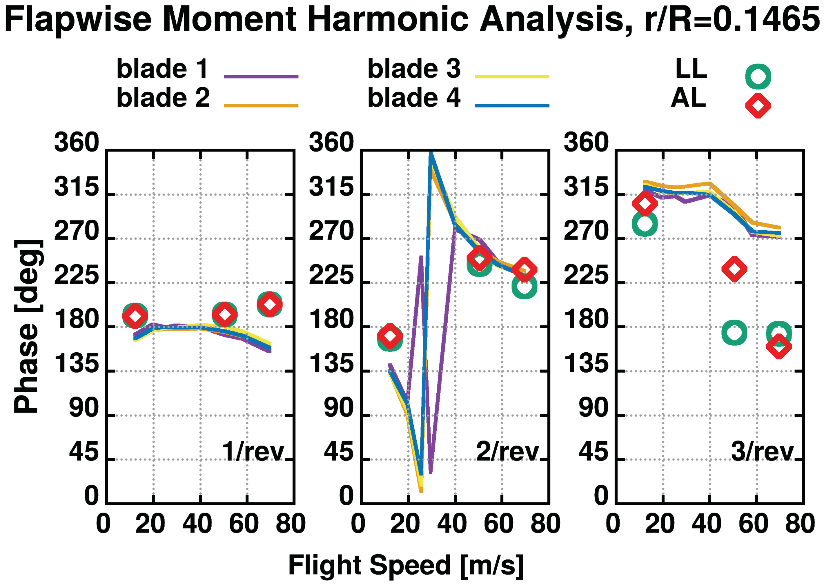
Figure 45.
Harmonic analysis of Flapwise bending moment. Phase of frequencies with the highest energy content.
Figure 45.
Harmonic analysis of Flapwise bending moment. Phase of frequencies with the highest energy content.
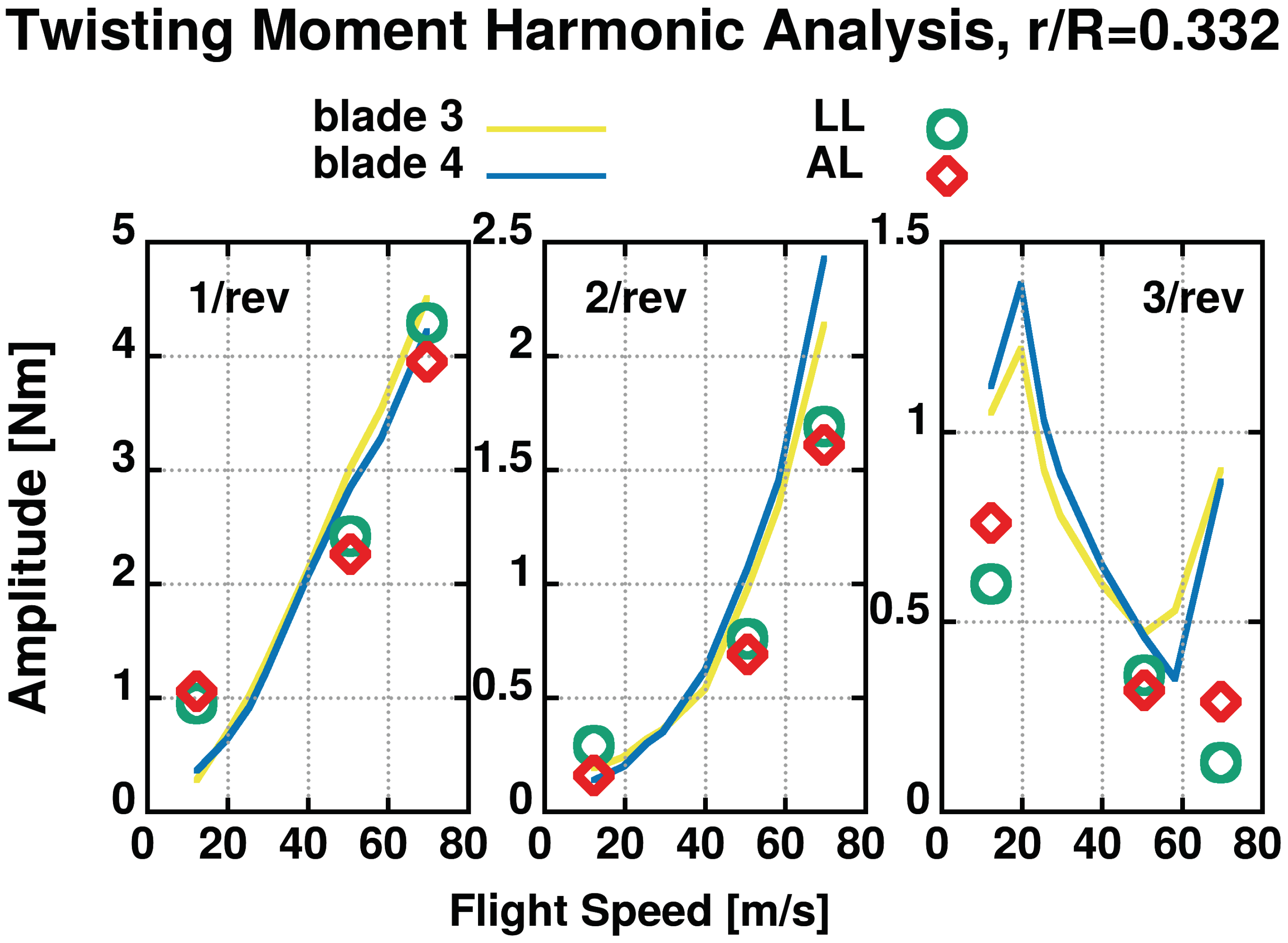
Figure 46.
Harmonic analysis of Twisting moment. Amplitude of frequencies with the highest energy content.
Figure 46.
Harmonic analysis of Twisting moment. Amplitude of frequencies with the highest energy content.
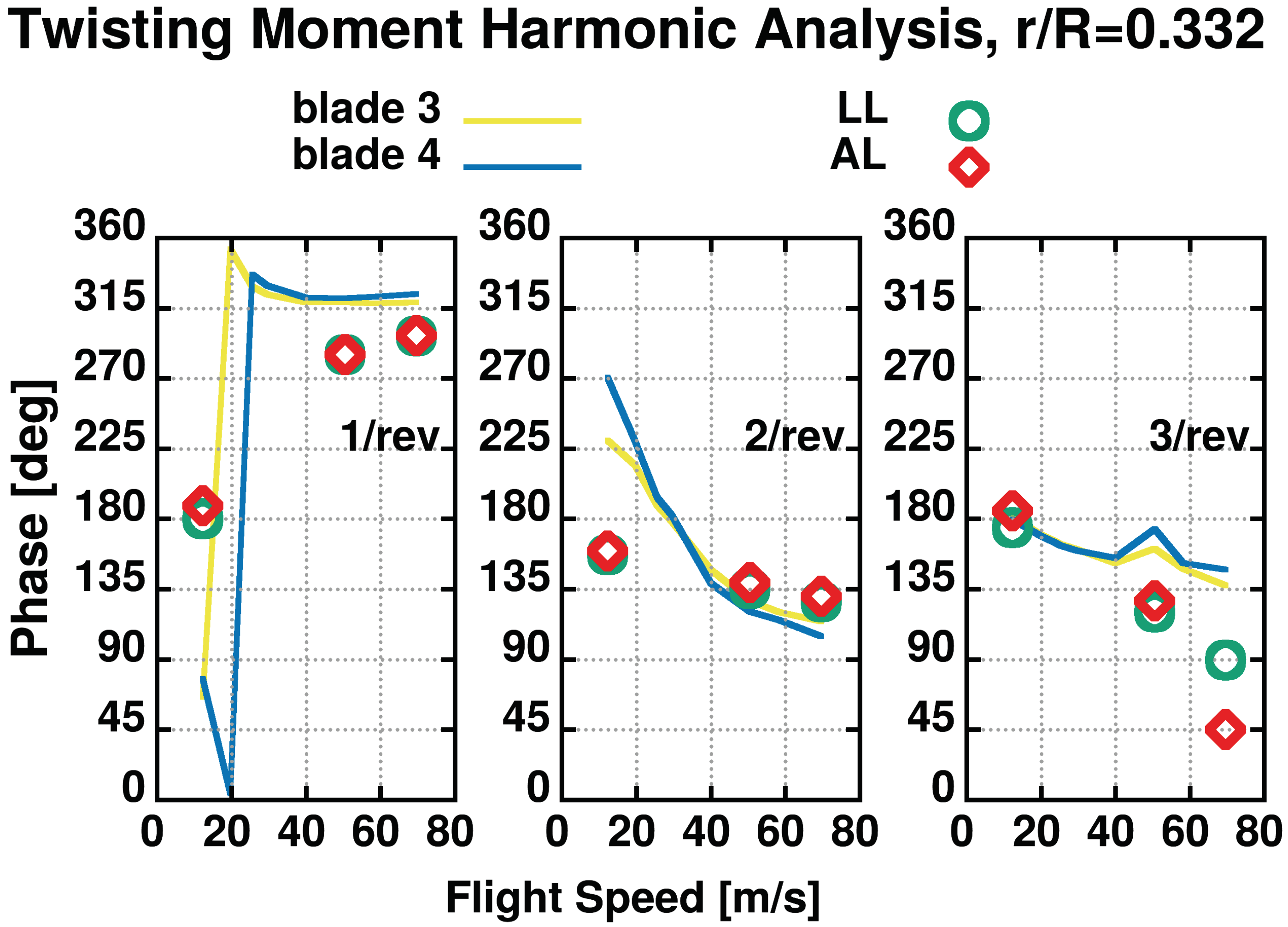
Figure 47.
Harmonic analysis of Twisting moment. Phase of frequencies with the highest energy content.
Figure 47.
Harmonic analysis of Twisting moment. Phase of frequencies with the highest energy content.
Table 1.
Variation of power [MW] with increasing the structured region characteristic length [m]. Reference power corresponds to minimum value .
Table 1.
Variation of power [MW] with increasing the structured region characteristic length [m]. Reference power corresponds to minimum value .
| | | | |
|---|
| | | |
| | | |
| | | |
| | | |
| | | |
| 7.921 MW | 9.202 MW | 9.362 MW |
Table 2.
Variation of power [MW] with increasing blade grid size [m]. Reference power corresponds to minimum value .
Table 2.
Variation of power [MW] with increasing blade grid size [m]. Reference power corresponds to minimum value .
| | |
|---|
| |
| |
| |
| 9.286 MW |
Table 3.
Variation of power [MW] with increasing wake region characteristic length [m]. Reference power corresponds to minimum value .
Table 3.
Variation of power [MW] with increasing wake region characteristic length [m]. Reference power corresponds to minimum value .
| | |
|---|
| |
| |
| 9.202 MW |
Table 4.
Variation of power [MW] with increasing time-step [sec]. Reference power corresponds to minimum value .
Table 4.
Variation of power [MW] with increasing time-step [sec]. Reference power corresponds to minimum value .
| | |
|---|
| |
| |
| 9.631 MW |
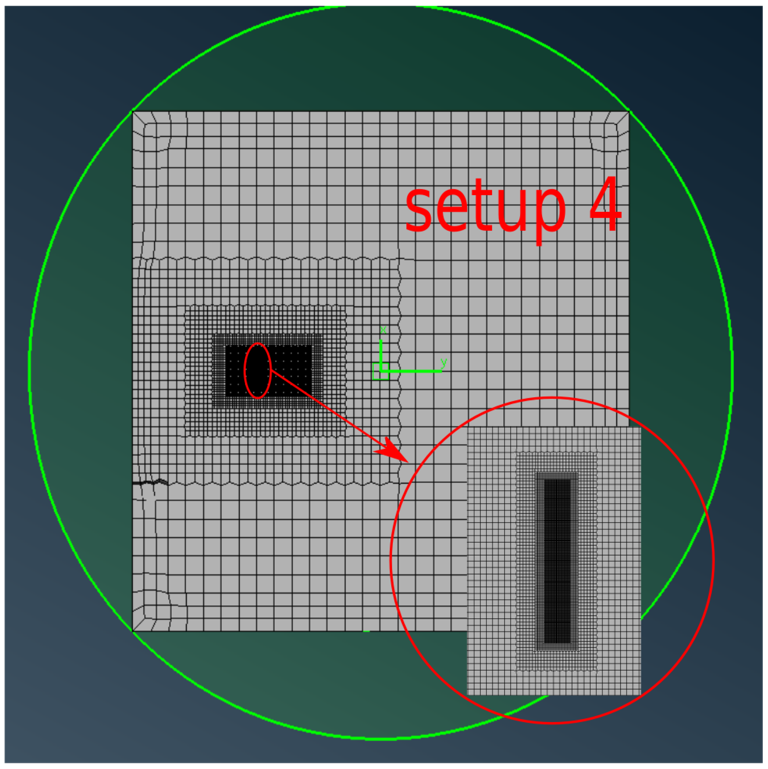
Table 5.
Variaton of power [MW] with different grid setup. Reference power corresponds to grid “setup4”.
Table 5.
Variaton of power [MW] with different grid setup. Reference power corresponds to grid “setup4”.
| | |
|---|
| |
| |
| |
| 9.607 MW |
Table 6.
Variation of thrust [kN] with increasing the structured region characteristic length [m]. Reference thrust corresponds to minimum value .
Table 6.
Variation of thrust [kN] with increasing the structured region characteristic length [m]. Reference thrust corresponds to minimum value .
| | |
|---|
| |
| |
| |
| 4.706 kN |
Table 7.
Variation of thrust [kN] with increasing blade grid size [m]. Reference thrust corresponds to minimum value .
Table 7.
Variation of thrust [kN] with increasing blade grid size [m]. Reference thrust corresponds to minimum value .
| | |
|---|
| |
| |
| 4.679 kN |
Table 8.
Variation of thrust [kN] with increasing time-step [s]. Reference thrust corresponds to minimum value .
Table 8.
Variation of thrust [kN] with increasing time-step [s]. Reference thrust corresponds to minimum value .
| | |
|---|
| |
| |
| |
| 4.683 kN |
Table 9.
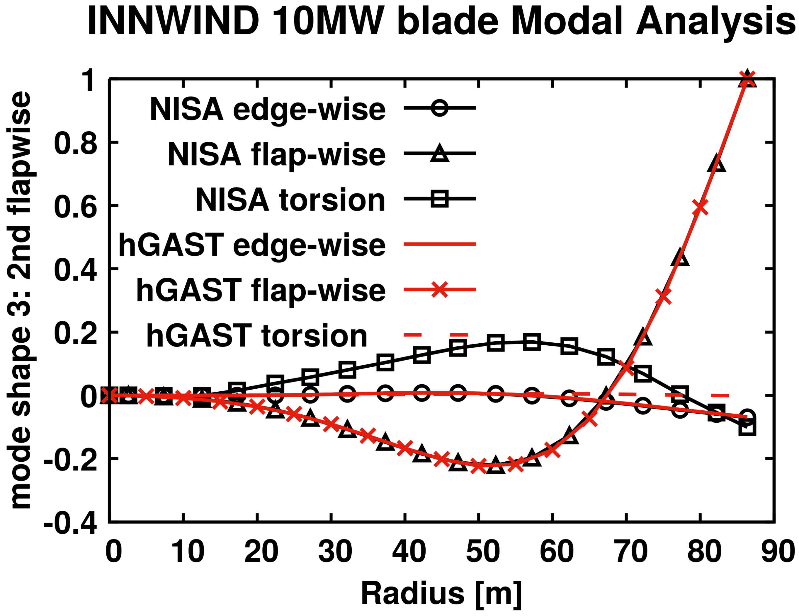
DTU 10MW blades natural frequencies. Comparison between different structural models used in WP2 of the INNWIND.EU project.
Table 9.
DTU 10MW blades natural frequencies. Comparison between different structural models used in WP2 of the INNWIND.EU project.
| Mode | hGAST | NEREA | Cp-Lambda | HAWC2 | NISA |
|---|
| 1st | | | | | |
| 1st | | | | | |
| 2nd | | | | | |
| 2nd | | | | | |
| 3rd | | | | | |
| 1st | | | — | | |
| 3rd | | | | | |
| 4th | | | | | — |
Table 10.
Out-of-plane bending moment of blade root at 8 m/s axial wind speed. Comparison between different aerodynamic models.
Table 10.
Out-of-plane bending moment of blade root at 8 m/s axial wind speed. Comparison between different aerodynamic models.
| | Mean Value [MNm] | Amplitude [MNm] | Phase [°] |
|---|
| BEM | | | 124 |
| LL | | | 160 |
| AL | | | 156 |
Table 11.
BO105 MR blade damping ratio at 1050 rpm.
Table 11.
BO105 MR blade damping ratio at 1050 rpm.
| Mode | Damping Ratio |
|---|
| 1st | |
| 1st | |
| 2nd | |
| 1st | |
| 3rd | |
| 2nd | |
| 4th | |
Table 12.
Mean values of blade structural loads.
Table 12.
Mean values of blade structural loads.
| | | | | | | | |
|---|
| | | - | | - | | | |
| 12.3 m/s | | | | | | | |
| | | - | - | | | | |
| | | - | | - | | | |
| 50.5 m/s | | | | | | | |
| | | - | - | | | | |
| | | - | | - | | | |
| 69.6 m/s | | | | | | | |
| | | - | - | | | | |
Table 13.
Mean values of blade deflections.
Table 13.
Mean values of blade deflections.
| | | | | | | | |
|---|
| | | | | | | | |
| 12.3 m/s | | | | | | | |
| | | | | | | | |
| | | | | | | | |
| 50.9 m/s | | | | | | | |
| | | | | | | | |
| | | | | | | | |
| 69.9 m/s | | | | | | | |
| | | | | | | | |


